Electrical Power Systems Quality, Second Edition phần 4 docx

charge voltage may be reduced only a few percent, the greatest benefit
of the scout scheme may be that it greatly reduces the rate of rise of
surge voltages entering the cable. These steep-fronted surges reflect off
the open point and frequently cause failures at the first or second pad-
mount transformer from the end. Because of lead lengths, arresters are
not always effective against such steep impulses. The scout scheme
practically eliminates these from the cable.
Many distribution feeders in densely populated areas will have scout
schemes by default. There are sufficient numbers of transformers that
there are already arresters on either side of the riser pole.
4.6 Managing Ferroresonance
Ferroresonance in a distribution system occurs mainly when a lightly
loaded, three-phase transformer becomes isolated on a cable with one
or two open phases. This can happen both accidentally and intention-
ally. Strategies for dealing with ferroresonance include
■
Preventing the open-phase condition
■
Damping the resonance with load
■
Limiting the overvoltages
■
Limiting cable lengths
■
Alternative cable-switching procedures
Most ferroresonance is a result of blown fuses in one or two of the
phases in response to faults, or some type of single-pole switching in
the primary circuit. A logical effective measure to guard against fer-
roresonance would be to use three-phase switching devices. For exam-
ple, a three-phase recloser or sectionalizer could be used at the riser
pole instead of fused cutouts. The main drawback is cost. Utilities could

not afford to do this at every riser pole, but this could be done in spe-
cial cases where there are particularly sensitive end users and frequent
fuse blowings.
Another strategy on troublesome cable drops is to simply replace the
fused cutouts with solid blades. This forces the upline recloser or
breaker to operate to clear faults on the cable. Of course, this subjects
many other utility customers to sustained interruptions when they
would have normally seen only a brief voltage sag. However, it is an
inexpensive way to handle the problem until a more permanent solu-
tion is implemented.
Manual, single-phase cable switching by pulling cutouts or cable
elbows is also a major source of ferroresonance. This is a particular
problem during new construction when there is a lot of activity and the
Transient Overvoltages 157
Transient Overvoltages
Downloaded from Digital Engineering Library @ McGraw-Hill (www.digitalengineeringlibrary.com)
Copyright © 2004 The McGraw-Hill Companies. All rights reserved.
Any use is subject to the Terms of Use as given at the website.
transformers are not yet loaded. Some utilities have reported that line
crews carry a “light board” or some other type of resistive load bank in
their trucks for use in cable-switching activity when the transformers
have no other load attached. One must be particularly careful when
switching delta-connected transformers; such transformers should be
protected because voltages may get extremely high. The common
grounded wye-wye pad-mounted transformer may not be damaged
internally if the exposure time is brief, although it may make consid-
erable noise. When switching manually, the goal should be to open or
close all three phases as promptly as possible.
Ferroresonance can generally be damped out by a relatively small
amount of resistive load, although there are exceptions. For the typ-

ical case with one phase open, a resistive load of 1 to 4 percent of the
transformer capacity can greatly reduce the effects of ferroreso-
nance. The amount of load required is dependent on the length of
cable and the design of the transformers. Also, the two-phase open
case is sometimes more difficult to dampen with load. Figure 4.38
shows the effect of loading on ferroresonance overvoltages for a
transformer connected to approximately 1.0 mi (1.61 km) of cable
with one phase open. This was a particularly difficult case that dam-
aged end-user equipment. Note the different characteristics of the
phases. The transformer was of a five-legged core design, and the
middle phase presents a condition that is more difficult to control
158 Chapter Four
0 5 10 15 20 25 30
1
1.2
1.4
1.6
1.8
2
2.2
2.4
2.6
2.8
3
A
B
C
Ferroresonant Voltage (per Unit)
Resistive Load @ 480 V BUS (% Transformer Capacity)
Figure 4.38 Example illustrating the impact of loading on ferroresonance.

Transient Overvoltages
Downloaded from Digital Engineering Library @ McGraw-Hill (www.digitalengineeringlibrary.com)
Copyright © 2004 The McGraw-Hill Companies. All rights reserved.
Any use is subject to the Terms of Use as given at the website.
with loading. Five percent resistive load reduces the overvoltage
from approximately 2.8 to 2 pu. The transformer would have to be
loaded approximately 20 to 25 percent of resistive equivalent load to
limit ferroresonance overvoltages to 125 percent, the commonly
accepted threshold. Since such a large load is required, a three-phase
recloser was used to switch the cable.
On many utility systems, arresters are not applied on every pad-
mounted distribution transformer due to costs. However, surge
arresters can be an effective tool for suppressing the effects of ferrores-
onance. This is particularly true for transformers with ungrounded pri-
mary connections where the voltages can easily reach 3 to 4 pu if
unchecked. Primary arresters will generally limit the voltages to 1.7 to
2.0 pu. There is some risk that arresters will fail if subjected to fer-
roresonance voltages for a long time. In fact, secondary arresters with
protective levels lower than the primary-side arresters are frequent
casualties of ferroresonance. Utility arresters are more robust, and
there often is relatively little energy involved. However, if line crews
encounter a transformer with arresters in ferroresonance, they should
always deenergize the unit and allow the arresters to cool. An over-
heated arrester could fail violently if suddenly reconnected to a source
with significant short-circuit capacity.
Ferroresonance occurs when the cable capacitance reaches a critical
value sufficient to resonate with the transformer inductance (see Fig.
4.11). Therefore, one strategy to minimize the risk of frequent ferroreso-
nance problems is to limit the length of cable runs. This is difficult to do
for transformers with delta primary connections because with the high

magnetizing reactance of modern transformers, ferroresonance can
occur for cable runs of less than 100 ft. The grounded wye-wye connec-
tion will generally tolerate a few hundred feet of cable without exceeding
125 percent voltage during single-phasing situations. The allowable
length of cable is also dependent on the voltage level with the general
trend being that the higher the system voltage, the shorter the cable.
However, modern trends in transformer designs with lower losses and
exciting currents are making it more difficult to completely avoid fer-
roresonance at all primary distribution voltage levels.
The location of switching when energizing or deenergizing a trans-
former can play a critical role in reducing the likelihood of ferroreso-
nance. Consider the two cable-transformer switching sequences in Fig.
4.39. Figure 4.39a depicts switching at the transformer terminals after
the underground cable is energized, i.e., switch L is closed first, fol-
lowed by switch R. Ferroresonance is less likely to occur since the
equivalent capacitance seen from an open phase after each phase of
switch R closes is the transformer’s internal capacitance and does not
involve the cable capacitance. Figure 4.39b depicts energization of the
Transient Overvoltages 159
Transient Overvoltages
Downloaded from Digital Engineering Library @ McGraw-Hill (www.digitalengineeringlibrary.com)
Copyright © 2004 The McGraw-Hill Companies. All rights reserved.
Any use is subject to the Terms of Use as given at the website.
transformer remotely from another point in the cable system. The
equivalent capacitance seen from switch L is the cable capacitance, and
the likelihood of ferroresonance is much greater. Thus, one of the com-
mon rules to prevent ferroresonance during cable switching is to switch
the transformer by pulling the elbows at the primary terminals. There
is little internal capacitance, and the losses of the transformers are
usually sufficient to prevent resonance with this small capacitance.

This is still a good general rule, although the reader should be aware
that some modern transformers violate this rule. Low-loss transform-
ers, particularly those built with an amorphous metal core, are prone
to ferroresonance with their internal capacitances.
4.7 Switching Transient Problems
with Loads
This section describes some transient problems related to loads and
load switching.
160 Chapter Four
(a)
underground cable
Switch L Switch R
(b)
underground cable
Switch L
Switch R
Figure 4.39 Switching at the transformer terminals (a) reduces the risk of iso-
lating the transformer on sufficient capacitance to cause ferroresonance as
opposed to (b) switching at some other location upline.
Transient Overvoltages
Downloaded from Digital Engineering Library @ McGraw-Hill (www.digitalengineeringlibrary.com)
Copyright © 2004 The McGraw-Hill Companies. All rights reserved.
Any use is subject to the Terms of Use as given at the website.
4.7.1 Nuisance tripping of ASDs
Most adjustable-speed drives typically use a voltage source inverter
(VSI) design with a capacitor in the dc link. The controls are sensitive
to dc overvoltages and may trip the drive at a level as low as 117 per-
cent. Since transient voltages due to utility capacitor switching typi-
cally exceed 130 percent, the probability of nuisance tripping of the
drive is high. One set of typical waveforms for this phenomenon is

shown in Fig. 4.40.
The most effective way to eliminate nuisance tripping of small drives
is to isolate them from the power system with ac line chokes. The addi-
tional series inductance of the choke will reduce the transient voltage
magnitude that appears at the input to the adjustable-speed drive.
Determining the precise inductor size required for a particular appli-
cation (based on utility capacitor size, transformer size, etc.) requires a
fairly detailed transient simulation. A series choke size of 3 percent
based on the drive kVA rating is usually sufficient.
4.7.2 Transients from load switching
Deenergizing inductive circuits with air-gap switches, such as relays
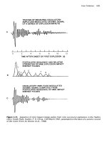
and contactors, can generate bursts of high-frequency impulses. Figure
4.41 shows an example. ANSI/IEEE C62.41-1991, Recommended
Practice for Surge Voltages in Low-Voltage AC Power Circuits, cites a
representative 15-ms burst composed of impulses having 5-ns rise
Transient Overvoltages 161
480-V Bus Voltage (phase-to-phase)
33.3 50.0 66.7 83.3 100.0 116.7
–1500
–1000
–500
0
500
1000
1500
Voltage (V)
Time (ms)
Figure 4.40 Effect of capacitor switching on adjustable-speed-drive ac current and dc
voltage.
Transient Overvoltages

Downloaded from Digital Engineering Library @ McGraw-Hill (www.digitalengineeringlibrary.com)
Copyright © 2004 The McGraw-Hill Companies. All rights reserved.
Any use is subject to the Terms of Use as given at the website.
times and 50-ns durations. There is very little energy in these types of
transient due to the short duration, but they can interfere with the
operation of electronic loads.
Such electrical fast transient (EFT) activity, producing spikes up to 1
kV, is frequently due to cycling motors, such as air conditioners and ele-
vators. Transients as high as 3 kV can be caused by operation of arc
welders and motor starters.
The duration of each impulse is short compared to the travel time of
building wiring, thus the propagation of these impulses through the
162 Chapter Four
ac Drive Current during Capacitor Switching
33.3 50.0 66.7 83.3 100.0 116.7
–300
–200
–100
0
100
200
300
Time (ms)
Current (A)
dc Link Voltage during Capacitor Switching
33.3 50.0 66.7 83.3 100.0 116.7
500
550
600
650

700
750
Time (ms)
Current (A)
Figure 4.40 (Continued)
Transient Overvoltages
Downloaded from Digital Engineering Library @ McGraw-Hill (www.digitalengineeringlibrary.com)
Copyright © 2004 The McGraw-Hill Companies. All rights reserved.
Any use is subject to the Terms of Use as given at the website.
wiring can be analyzed with traveling wave theory. The impulses atten-
uate very quickly as they propagate through a building. Therefore, in
most cases, the only protection needed is electrical separation. Physical
separation is also required because the high rate of rise allows these
transients to couple into nearby sensitive equipment.
EFT suppression may be required with extremely sensitive equip-
ment in close proximity to a disturbing load, such as a computer room.
High-frequency filters and isolation transformers can be used to pro-
tect against conduction of EFTs on power cables. Shielding is required
to prevent coupling into equipment and data lines.
4.7.3 Transformer energizing
Energizing a transformer produces inrush currents that are rich in
harmonic components for a period lasting up to 1 s. If the system has a
parallel resonance near one of the harmonic frequencies, a dynamic
overvoltage condition results that can cause failure of arresters and
problems with sensitive equipment. This problem can occur when large
transformers are energized simultaneously with large power factor cor-
rection capacitor banks in industrial facilities. The equivalent circuit is
shown in Fig. 4.42. A dynamic overvoltage waveform caused by a third-
harmonic resonance in the circuit is shown in Fig. 4.43. After the
expected initial transient, the voltage again swells to nearly 150 per-

cent for many cycles until the losses and load damp out the oscillations.
This can place severe stress on some arresters and has been known to
significantly shorten the life of capacitors.
Transient Overvoltages 163
400V
0V
–400V
200 V/div VERTICAL 102.4 ␮s/div HORIZ
1000V
0V
–1000V
500.0 V/div VERTICAL 5.0 ms/div HORIZ
Figure 4.41 Fast transients caused by deenergizing an inductive load.
Transient Overvoltages
Downloaded from Digital Engineering Library @ McGraw-Hill (www.digitalengineeringlibrary.com)
Copyright © 2004 The McGraw-Hill Companies. All rights reserved.
Any use is subject to the Terms of Use as given at the website.
This form of dynamic overvoltage problem can often be eliminated
simply by not energizing the capacitor and transformer together. One
plant solved the problem by energizing the transformer first and not
energizing the capacitor until load was about to be connected to the
transformer.
4.8 Computer Tools for Transients Analysis
The most widely used computer programs for transients analysis of
power systems are the Electromagnetic Transients Program, com-
monly known as EMTP, and its derivatives such as the Alternate
Transients Program (ATP). EMTP was originally developed by
Hermann W. Dommel at the Bonneville Power Administration (BPA) in
the late 1960s
15

and has been continuously upgraded since. One of the
reasons this program is popular is its low cost due to some versions
being in the public domain. Some of the simulations presented in this
164 Chapter Four
Figure 4.42 Energizing a capacitor and transformer
simultaneously can lead to dynamic overvoltages.
–2
–1
0
1
2
0 200 400 600 800
Phase A
Time (ms)
Voltage (V pu)
Figure 4.43 Dynamic overvoltages during transformer energizing.
Transient Overvoltages
Downloaded from Digital Engineering Library @ McGraw-Hill (www.digitalengineeringlibrary.com)
Copyright © 2004 The McGraw-Hill Companies. All rights reserved.
Any use is subject to the Terms of Use as given at the website.
book have been performed with a commercial analysis tool known as
PSCAD/EMTDC, a program developed by the Manitoba HVDC
Research Center. This program features a very sophisticated graphical
user interface that enables the user to be very productive in this diffi-
cult analysis. Some power system analysts use computer programs
developed more for the analysis of electronic circuits, such as the well-
known SPICE program
16
and its derivatives.
Although the programs just discussed continue to be used exten-

sively, there are now many other capable programs available. We will
not attempt to list each one because there are so many and, also, at the
present rate of software development, any such list would soon be out-
dated. The reader is referred to the Internet since all vendors of this
type of software maintain websites.
Nearly all the tools for power systems solve the problem in the time
domain, re-creating the waveform point by point. A few programs solve
in the frequency domain and use the Fourier transform to convert to
the time domain. Unfortunately, this essentially restricts the address-
able problems to linear circuits. Time-domain solution is required to
model nonlinear elements such as surge arresters and transformer
magnetizing characteristics. The penalty for this extra capability is
longer solution times, which with modern computers becomes less of a
problem each day.
It takes considerably more modeling expertise to perform electro-
magnetic transients studies than to perform more common power sys-
tem analyses such as of the power flow or of a short circuit. Therefore,
this task is usually relegated to a few specialists within the utility orga-
nization or to consultants.
While transients programs for electronic circuit analysis may formu-
late the problem in any number of ways, power systems analysts
almost uniformly favor some type of nodal admittance formulation. For
one thing, the system admittance matrix is sparse allowing the use of
very fast and efficient sparsity techniques for solving large problems.
Also, the nodal admittance formulation reflects how most power engi-
neers view the power system, with series and shunt elements con-
nected to buses where the voltage is measured with respect to a single
reference.
To obtain conductances for elements described by differential equa-
tions, transients programs discretize the equations with an appropri-

ate numerical integration formula. The simple trapezoidal rule method
appears to be the most commonly used, but there are also a variety of
Runge-Kutta and other formulations used. Nonlinearities are handled
by iterative solution methods. Some programs include the nonlineari-
ties in the general formulation, while others, such as those that follow
Transient Overvoltages 165
Transient Overvoltages
Downloaded from Digital Engineering Library @ McGraw-Hill (www.digitalengineeringlibrary.com)
Copyright © 2004 The McGraw-Hill Companies. All rights reserved.
Any use is subject to the Terms of Use as given at the website.
the EMTP methodology, separate the linear and nonlinear portions of
the circuit to achieve faster solutions. This impairs the ability of the
program to solve some classes of nonlinear problems but is not usually
a significant constraint for most power system problems.
4.9 References
1. Electrical Transmission and Distribution Reference Book, 4th ed., Westinghouse
Electric Corporation, East Pittsburgh, Pa., 1964.
2. Electrical Distribution-System Protection, 3d ed., Cooper Power Systems,
Franksville, Wis., 1990.
3. K. Berger, R. B. Anderson, H. Kroninger, “Parameters of Lightning Flashes, “
Electra, No. 41, July 1975, pp. 23–27.
4. R. Morrison, W. H. Lewis, Grounding and Shielding in Facilities, John Wiley & Sons,
New York, 1990.
5. G. L. Goedde, L. J. Kojovic, M. B. Marz, J. J. Woodworth, “Series-Graded Gapped
Arrester Provides Reliable Overvoltage Protection in Distribution Systems,”
Conference Record, 2001 IEEE Power Engineering Society Winter Meeting, Vol. 3,
2001, pp. 1122–1127.
6. Randall A. Stansberry, “Protecting Distribution Circuits: Overhead Shield Wire ver-
sus Lightning Surge Arresters,” Transmission & Distribution, April 1991, pp. 56ff.
7. IEEE Transformers Committee, “Secondary (Low-Side) Surges in Distribution

Transformers,” Proceedings of the 1991 IEEE PES Transmission and Distribution
Conference, Dallas, September 1991, pp. 998–1008.
8. C. W. Plummer, et al., “Reduction in Distribution Transformer Failure Rates and
Nuisance Outages Using Improved Lightning Protection Concepts,” Proceedings of
the 1994 IEEE PES Transmission and Distribution Conference, Chicago, April 1994,
pp. 411–416.
9. G. L. Goedde, L. A. Kojovic, J. J. Woodworth, “Surge Arrester Characteristics That
Provide Reliable Overvoltage Protection in Distribution and Low-Voltage Systems,”
Conference Record, 2000 IEEE Power Engineering Society Summer Meeting, Vol. 4,
2000, pp. 2375–2380.
10. P. Barker, R. Mancao, D. Kvaltine, D. Parrish, “Characteristics of Lightning Surges
Measured at Metal Oxide Distribution Arresters,” IEEE Transactions on Power
Delivery, October 1993, pp. 301–310.
11. R. H. Hopkinson, “Better Surge Protection Extends URD Cable Life,” IEEE
Transactions on Power Apparatus and Systems, Vol. PAS-103, 1984, pp. 2827–2834.
12. G. L. Goedde, R. C Dugan, L. D. Rowe, “Full Scale Lightning Surge Tests of
Distribution Transformers and Secondary Systems,” Proceedings of the 1991 IEEE
PES Transmission and Distribution Conference, Dallas, September 1991, pp.
691–697.
13. S. S. Kershaw, Jr., “Surge Protection for High Voltage Underground Distribution
Circuits,” Conference Record, IEEE Conference on Underground Distribution,
Detroit, September 1971, pp. 370–384.
14. M. B. Marz, T. E. Royster, C. M. Wahlgren, “A Utility’s Approach to the Application
of Scout Arresters for Overvoltage Protection of Underground Distribution Circuits,”
1994 IEEE Transmission and Distribution Conference Record, Chicago, April 1994,
pp. 417–425.
15. H. W. Dommel, “Digital Computer Solution of Electromagnetic Transients in Single
and Multiphase Networks,” IEEE Transactions on Power Apparatus and Systems,
Vol. PAS-88, April 1969, pp. 388–399.
16. L. W. Nagel, “SPICE2: A Computer Program to Simulate Semiconductor Circuits,”

Ph. D. thesis, University of California, Berkeley, Electronics Research Laboratory,
No. ERL-M520, May 1975.
166 Chapter Four
Transient Overvoltages
Downloaded from Digital Engineering Library @ McGraw-Hill (www.digitalengineeringlibrary.com)
Copyright © 2004 The McGraw-Hill Companies. All rights reserved.
Any use is subject to the Terms of Use as given at the website.
167
Fundamentals of Harmonics
A good assumption for most utilities in the United States is that the
sine-wave voltage generated in central power stations is very good. In
most areas, the voltage found on transmission systems typically has
much less than 1.0 percent distortion. However, the distortion
increases closer to the load. At some loads, the current waveform
barely resembles a sine wave. Electronic power converters can chop
the current into seemingly arbitrary waveforms.
While there are a few cases where the distortion is random, most dis-
tortion is periodic, or an integer multiple of the power system funda-
mental frequency. That is, the current waveform is nearly the same
cycle after cycle, changing very slowly, if at all. This has given rise to
the widespread use of the term harmonics to describe distortion of the
waveform. This term must be carefully qualified to make sense. This
chapter and Chap. 6 remove some of the mystery of harmonics in power
systems.
When electronic power converters first became commonplace in the
late 1970s, many utility engineers became quite concerned about the
ability of the power system to accommodate the harmonic distortion.
Many dire predictions were made about the fate of power systems if
these devices were permitted to exist. While some of these concerns
were probably overstated, the field of power quality analysis owes a

great debt of gratitude to these people because their concern over this
“new” problem of harmonics sparked the research that has eventually
led to much of the knowledge about all aspects of power quality.
To some, harmonic distortion is still the most significant power qual-
ity problem. It is not hard to understand how an engineer faced with a
difficult harmonics problem can come to hold that opinion. Harmonics
problems counter many of the conventional rules of power system
Chapter
5
Source: Electrical Power Systems Quality
Downloaded from Digital Engineering Library @ McGraw-Hill (www.digitalengineeringlibrary.com)
Copyright © 2004 The McGraw-Hill Companies. All rights reserved.
Any use is subject to the Terms of Use as given at the website.
design and operation that consider only the fundamental frequency.
Therefore, the engineer is faced with unfamiliar phenomena that
require unfamiliar tools to analyze and unfamiliar equipment to solve.
Although harmonic problems can be difficult, they are not actually very
numerous on utility systems. Only a few percent of utility distribution
feeders in the United States have a sufficiently severe harmonics prob-
lem to require attention.
In contrast, voltage sags and interruptions are nearly universal to
every feeder and represent the most numerous and significant power
quality deviations. The end-user sector suffers more from harmonic
problems than does the utility sector. Industrial users with adjustable-
speed drives, arc furnaces, induction furnaces, and the like are much
more susceptible to problems stemming from harmonic distortion.
Harmonic distortion is not a new phenomenon on power systems.
Concern over distortion has ebbed and flowed a number of times dur-
ing the history of ac electric power systems. Scanning the technical lit-
erature of the 1930s and 1940s, one will notice many articles on the

subject. At that time the primary sources were the transformers and
the primary problem was inductive interference with open-wire tele-
phone systems. The forerunners of modern arc lighting were being
introduced and were causing quite a stir because of their harmonic con-
tent—not unlike the stir caused by electronic power converters in more
recent times.
Fortunately, if the system is properly sized to handle the power
demands of the load, there is a low probability that harmonics will
cause a problem with the power system, although they may cause prob-
lems with telecommunications. The power system problems arise most
frequently when the capacitance in the system results in resonance at
a critical harmonic frequency that dramatically increases the distor-
tion above normal amounts. While these problems occur on utility sys-
tems, the most severe cases are usually found in industrial power
systems because of the higher degree of resonance achieved.
5.1 Harmonic Distortion
Harmonic distortion is caused by nonlinear devices in the power sys-
tem. A nonlinear device is one in which the current is not proportional
to the applied voltage. Figure 5.1 illustrates this concept by the case of
a sinusoidal voltage applied to a simple nonlinear resistor in which the
voltage and current vary according to the curve shown. While the
applied voltage is perfectly sinusoidal, the resulting current is dis-
torted. Increasing the voltage by a few percent may cause the current
to double and take on a different waveshape. This is the source of most
harmonic distortion in a power system.
168 Chapter Five
Fundamentals of Harmonics
Downloaded from Digital Engineering Library @ McGraw-Hill (www.digitalengineeringlibrary.com)
Copyright © 2004 The McGraw-Hill Companies. All rights reserved.
Any use is subject to the Terms of Use as given at the website.

Figure 5.2 illustrates that any periodic, distorted waveform can be
expressed as a sum of sinusoids. When a waveform is identical from one
cycle to the next, it can be represented as a sum of pure sine waves in
which the frequency of each sinusoid is an integer multiple of the fun-
damental frequency of the distorted wave. This multiple is called a har-
monic of the fundamental, hence the name of this subject matter. The
sum of sinusoids is referred to as a Fourier series, named after the great
mathematician who discovered the concept.
Because of the above property, the Fourier series concept is univer-
sally applied in analyzing harmonic problems. The system can now be
analyzed separately at each harmonic. In addition, finding the system
response of a sinusoid of each harmonic individually is much more
straightforward compared to that with the entire distorted waveforms.
The outputs at each frequency are then combined to form a new Fourier
series, from which the output waveform may be computed, if desired.
Often, only the magnitudes of the harmonics are of interest.
When both the positive and negative half cycles of a waveform have
identical shapes, the Fourier series contains only odd harmonics. This
offers a further simplification for most power system studies because
most common harmonic-producing devices look the same to both polari-
ties. In fact, the presence of even harmonics is often a clue that there is
something wrong—either with the load equipment or with the transducer
used to make the measurement. There are notable exceptions to this such
as half-wave rectifiers and arc furnaces when the arc is random.
Fundamentals of Harmonics 169
V(t)
I(t)
V
I
Nonlinear Resistor

Figure 5.1 Current distortion caused by nonlinear resistance.
Fundamentals of Harmonics
Downloaded from Digital Engineering Library @ McGraw-Hill (www.digitalengineeringlibrary.com)
Copyright © 2004 The McGraw-Hill Companies. All rights reserved.
Any use is subject to the Terms of Use as given at the website.
·
+
+
+
+
+
+
·
·
+
60 Hz
(h = 1)
300 Hz
(h = 5)
420 Hz
(h = 7)
540 Hz
(h = 9)
660 Hz
(h = 11)
780 Hz
(h = 13)
180 Hz
(h = 3)
Figure 5.2 Fourier series representation of a distorted waveform.

170 Chapter Five
Usually, the higher-order harmonics (above the range of the 25th to
50th, depending on the system) are negligible for power system
analysis. While they may cause interference with low-power elec-
tronic devices, they are usually not damaging to the power system. It
is also difficult to collect sufficiently accurate data to model power
systems at these frequencies. A common exception to this occurs when
there are system resonances in the range of frequencies. These reso-
nances can be excited by notching or switching transients in elec-
tronic power converters. This causes voltage waveforms with multiple
zero crossings which disrupt timing circuits. These resonances gener-
ally occur on systems with underground cable but no power factor cor-
rection capacitors.
If the power system is depicted as series and shunt elements, as is
the conventional practice, the vast majority of the nonlinearities in the
system are found in shunt elements (i.e., loads). The series impedance
of the power delivery system (i.e., the short-circuit impedance between
the source and the load) is remarkably linear. In transformers, also, the
source of harmonics is the shunt branch (magnetizing impedance) of
the common “T” model; the leakage impedance is linear. Thus, the main
sources of harmonic distortion will ultimately be end-user loads. This
is not to say that all end users who experience harmonic distortion will
themselves have significant sources of harmonics, but that the har-
Fundamentals of Harmonics
Downloaded from Digital Engineering Library @ McGraw-Hill (www.digitalengineeringlibrary.com)
Copyright © 2004 The McGraw-Hill Companies. All rights reserved.
Any use is subject to the Terms of Use as given at the website.
Fundamentals of Harmonics 171
monic distortion generally originates with some end-user’s load or com-
bination of loads.

5.2 Voltage versus Current Distortion
The word harmonics is often used by itself without further qualifica-
tion. For example, it is common to hear that an adjustable-speed drive
or an induction furnace can’t operate properly because of harmonics.
What does that mean? Generally, it could mean one of the following
three things:
1. The harmonic voltages are too great (the voltage too distorted) for
the control to properly determine firing angles.
2. The harmonic currents are too great for the capacity of some device
in the power supply system such as a transformer, and the machine
must be operated at a lower than rated power.
3. The harmonic voltages are too great because the harmonic currents
produced by the device are too great for the given system condition.
As suggested by this list, there are separate causes and effects for volt-
ages and currents as well as some relationship between them. Thus,
the term harmonics by itself is inadequate to definitively describe a
problem.
Nonlinear loads appear to be sources of harmonic current in shunt
with and injecting harmonic currents into the power system. For nearly
all analyses, it is sufficient to treat these harmonic-producing loads
simply as current sources. There are exceptions to this as will be
described later.
As Fig. 5.3 shows, voltage distortion is the result of distorted cur-
rents passing through the linear, series impedance of the power deliv-
ery system, although, assuming that the source bus is ultimately a
pure sinusoid, there is a nonlinear load that draws a distorted current.
The harmonic currents passing through the impedance of the system
Pure
Sinusoid
Distorted Load

Current
Distorted Voltage
+
–
(Voltage Drop)
Figure 5.3 Harmonic currents flowing through the system impedance result in
harmonic voltages at the load.
Fundamentals of Harmonics
Downloaded from Digital Engineering Library @ McGraw-Hill (www.digitalengineeringlibrary.com)
Copyright © 2004 The McGraw-Hill Companies. All rights reserved.
Any use is subject to the Terms of Use as given at the website.
cause a voltage drop for each harmonic. This results in voltage har-
monics appearing at the load bus. The amount of voltage distortion
depends on the impedance and the current. Assuming the load bus dis-
tortion stays within reasonable limits (e.g., less than 5 percent), the
amount of harmonic current produced by the load is generally constant.
While the load current harmonics ultimately cause the voltage dis-
tortion, it should be noted that load has no control over the voltage dis-
tortion. The same load put in two different locations on the power
system will result in two different voltage distortion values.
Recognition of this fact is the basis for the division of responsibilities
for harmonic control that are found in standards such as IEEE
Standard 519-1992, Recommended Practices and Requirements for
Harmonic Control in Electrical Power Systems:
1. The control over the amount of harmonic current injected into the
system takes place at the end-use application.
2. Assuming the harmonic current injection is within reasonable lim-
its, the control over the voltage distortion is exercised by the entity
having control over the system impedance, which is often the utility.
One must be careful when describing harmonic phenomena to under-

stand that there are distinct differences between the causes and effects
of harmonic voltages and currents. The use of the term harmonics
should be qualified accordingly. By popular convention in the power
industry, the majority of times when the term is used by itself to refer
to the load apparatus, the speaker is referring to the harmonic cur-
rents. When referring to the utility system, the voltages are generally
the subject. To be safe, make a habit of asking for clarification.
5.3 Harmonics versus Transients
Harmonic distortion is blamed for many power quality disturbances
that are actually transients. A measurement of the event may show a
distorted waveform with obvious high-frequency components.
Although transient disturbances contain high-frequency components,
transients and harmonics are distinctly different phenomena and are
analyzed differently. Transient waveforms exhibit the high frequencies
only briefly after there has been an abrupt change in the power system.
The frequencies are not necessarily harmonics; they are the natural
frequencies of the system at the time of the switching operation. These
frequencies have no relation to the system fundamental frequency.
Harmonics, by definition, occur in the steady state and are integer
multiples of the fundamental frequency. The waveform distortion that
produces the harmonics is present continually, or at least for several
172 Chapter Five
Fundamentals of Harmonics
Downloaded from Digital Engineering Library @ McGraw-Hill (www.digitalengineeringlibrary.com)
Copyright © 2004 The McGraw-Hill Companies. All rights reserved.
Any use is subject to the Terms of Use as given at the website.
seconds. Transients are usually dissipated within a few cycles. Trans-
ients are associated with changes in the system such as switching of a
capacitor bank. Harmonics are associated with the continuing opera-
tion of a load.

One case in which the distinction is blurred is transformer energiza-
tion. This is a transient event but can produce considerable waveform
distortion for many seconds and has been known to excite system res-
onances.
5.4 Power System Quantities under
Nonsinusoidal Conditions
Traditional power system quantities such as rms, power (reactive,
active, apparent), power factor, and phase sequences are defined for the
fundamental frequency context in a pure sinusoidal condition. In the
presence of harmonic distortion the power system no longer operates in
a sinusoidal condition, and unfortunately many of the simplifications
power engineers use for the fundamental frequency analysis do not
apply.
5.4.1 Active, reactive, and apparent power
There are three standard quantities associated with power:
■
Apparent power S [voltampere (VA)]. The product of the rms voltage
and current.
■
Active power P [watt (W)]. The average rate of delivery of energy.
■
Reactive power Q [voltampere-reactive] (var)]. The portion of the
apparent power that is out of phase, or in quadrature, with the active
power.
The apparent power S applies to both sinusoidal and nonsinusoidal
conditions. The apparent power can be written as follows:
S ϭ V
rms
ϫ I
rms

(5.1)
where V
rms
and I
rms
are the rms values of the voltage and current. In a
sinusoidal condition both the voltage and current waveforms contain
only the fundamental frequency component; thus the rms values can be
expressed simply as
V
rms
ϭ V
1
and I
rms
ϭ I
1
(5.2)
1
ᎏ
͙2
ෆ
1
ᎏ
͙2
ෆ
Fundamentals of Harmonics 173
Fundamentals of Harmonics
Downloaded from Digital Engineering Library @ McGraw-Hill (www.digitalengineeringlibrary.com)
Copyright © 2004 The McGraw-Hill Companies. All rights reserved.

Any use is subject to the Terms of Use as given at the website.
where V
1
and I
1
are the amplitude of voltage and current waveforms,
respectively. The subscript “1” denotes quantities in the fundamental
frequency. In a nonsinusoidal condition a harmonically distorted wave-
form is made up of sinusoids of harmonic frequencies with different
amplitudes as shown in Fig. 5.2. The rms values of the waveforms are
computed as the square root of the sum of rms squares of all individual
components, i.e.,
V
rms
ϭ
Ί
Α
h
max
h ϭ 1
΂
๶
๶
V
h
΃
2
๶
ϭ
͙

V
1
2
ϩ
ෆ
V
2
2
ϩ
ෆ
V
3
2
ϩ
ෆ
…
ϩ V
ෆ
2
h
max
ෆ
(5.3)
I
rms
ϭ
Ί
Α
h
max

h ϭ 1
΂
๶
๶
I
h
΃
2
๶
ϭ
͙
I
1
2
ϩ I
ෆ
2
2
ϩ I
3
ෆ
2
ϩ
…
ෆ
ϩ I
2
h
m
ෆ

ax
ෆ
(5.4)
where V
h
and I
h
are the amplitude of a waveform at the harmonic com-
ponent h. In the sinusoidal condition, harmonic components of V
h
and
I
h
are all zero, and only V
1
and I
1
remain. Equations (5.3) and (5.4) sim-
plify to Eq. (5.2).
The active power P is also commonly referred to as the average
power, real power, or true power. It represents useful power expended
by loads to perform real work, i.e., to convert electric energy to other
forms of energy. Real work performed by an incandescent light bulb is
to convert electric energy into light and heat. In electric power, real
work is performed for the portion of the current that is in phase with
the voltage. No real work will result from the portion where the current
is not in phase with the voltage. The active power is the rate at which
energy is expended, dissipated, or consumed by the load and is mea-
sured in units of watts. P can be computed by averaging the product of
the instantaneous voltage and current, i.e.,

P ϭ
͵
T
0
v(t) i(t) dt (5.5)
Equation (5.5) is valid for both sinusoidal and nonsinusoidal condi-
tions. For the sinusoidal condition, P resolves to the familiar form,
P ϭ cos ␪
1
ϭ V
1rms
I
1rms
cos ␪
1
ϭ S cos ␪
1
(5.6)
where ␪
1
is the phase angle between voltage and current at the funda-
mental frequency. Equation (5.6) indicates that the average active
V
1
I
1
ᎏ
2
1
ᎏ

T
1
ᎏ
͙2
ෆ
1
ᎏ
͙2
ෆ
1
ᎏ
͙2
ෆ
1
ᎏ
͙2
ෆ
174 Chapter Five
h
h
Fundamentals of Harmonics
Downloaded from Digital Engineering Library @ McGraw-Hill (www.digitalengineeringlibrary.com)
Copyright © 2004 The McGraw-Hill Companies. All rights reserved.
Any use is subject to the Terms of Use as given at the website.
power is a function only of the fundamental frequency quantities. In
the nonsinusoidal case, the computation of the active power must
include contributions from all harmonic components; thus it is the sum
of active power at each harmonic. Furthermore, because the voltage
distortion is generally very low on power systems (less than 5 percent),
Eq. (5.6) is a good approximation regardless of how distorted the cur-

rent is. This approximation cannot be applied when computing the
apparent and reactive power. These two quantities are greatly influ-
enced by the distortion. The apparent power S is a measure of the
potential impact of the load on the thermal capability of the system. It
is proportional to the rms of the distorted current, and its computation
is straightforward, although slightly more complicated than the sinu-
soidal case. Also, many current probes can now directly report the true
rms value of a distorted waveform.
The reactive power is a type of power that does no real work and is
generally associated with reactive elements (inductors and capacitors).
For example, the inductance of a load such as a motor causes the load
current to lag behind the voltage. Power appearing across the induc-
tance sloshes back and forth between the inductance itself and the
power system source, producing no net work. For this reason it is called
imaginary or reactive power since no power is dissipated or expended.
It is expressed in units of vars. In the sinusoidal case, the reactive
power is simply defined as
Q ϭ S sin ␪
1
ϭ sin ␪
1
ϭ V
1rms
I
1rms
sin ␪
1
(5.7)
which is the portion of power in quadrature with the active power
shown in Eq. (5.6). Figure 5.4 summarizes the relationship between P,

Q, and S in sinusoidal condition.
There is some disagreement among harmonics analysts on how to
define Q in the presence of harmonic distortion. If it were not for the
fact that many utilities measure Q and compute demand billing from
the power factor computed by Q, it might be a moot point. It is more
important to determine P and S; P defines how much active power is
being consumed, while S defines the capacity of the power system
required to deliver P. Q is not actually very useful by itself. However,
Q
1
, the traditional reactive power component at fundamental fre-
quency, may be used to size shunt capacitors.
The reactive power when distortion is present has another interest-
ing peculiarity. In fact, it may not be appropriate to call it reactive
power. The concept of var flow in the power system is deeply ingrained
in the minds of most power engineers. What many do not realize is
that this concept is valid only in the sinusoidal steady state. When dis-
V
1
I
1
ᎏ
2
Fundamentals of Harmonics 175
Fundamentals of Harmonics
Downloaded from Digital Engineering Library @ McGraw-Hill (www.digitalengineeringlibrary.com)
Copyright © 2004 The McGraw-Hill Companies. All rights reserved.
Any use is subject to the Terms of Use as given at the website.
tortion is present, the component of S that remains after P is taken out
is not conserved—that is, it does not sum to zero at a node. Power

quantities are presumed to flow around the system in a conservative
manner.
This does not imply that P is not conserved or that current is not
conserved because the conservation of energy and Kirchoff’s current
laws are still applicable for any waveform. The reactive components
actually sum in quadrature (square root of the sum of the squares).
This has prompted some analysts to propose that Q be used to denote
the reactive components that are conserved and introduce a new quan-
tity for the components that are not. Many call this quantity D, for dis-
tortion power or, simply, distortion voltamperes. It has units of
voltamperes, but it may not be strictly appropriate to refer to this
quantity as power, because it does not flow through the system as
power is assumed to do. In this concept, Q consists of the sum of the
traditional reactive power values at each frequency. D represents all
cross products of voltage and current at different frequencies, which
yield no average power. P, Q, D, and S are related as follows, using the
definitions for S and P previously given in Eqs. (5.1) and (5.5) as a
starting point:
S ϭ
͙
P
2
ϩ Q
ෆ
2
ϩ D
2
ෆ
Q ϭ
Α

k
V
k
I
k
sin ␪
k
(5.8)
Therefore, D can be determined after S, P, and Q by
D ϭ ͙S
2
Ϫ P
ෆ
2
Ϫ Q
2
ෆ
(5.9)
Some prefer to use a three-dimensional vector chart to demonstrate the
relationships of the components as shown in Fig. 5.5. P and Q con-
176 Chapter Five
S
P
Q
Figure 5.4 Relationship between
P, Q , and S in sinusoidal condition.
Fundamentals of Harmonics
Downloaded from Digital Engineering Library @ McGraw-Hill (www.digitalengineeringlibrary.com)
Copyright © 2004 The McGraw-Hill Companies. All rights reserved.
Any use is subject to the Terms of Use as given at the website.

tribute the traditional sinusoidal components to S, while D represents
the additional contribution to the apparent power by the harmonics.
5.4.2 Power factor: displacement and true
Power factor (PF) is a ratio of useful power to perform real work (active
power) to the power supplied by a utility (apparent power), i.e.,
PF ϭ (5.10)
In other words, the power factor ratio measures the percentage of power
expended for its intended use. Power factor ranges from zero to unity. A
load with a power factor of 0.9 lagging denotes that the load can effectively
expend 90 percent of the apparent power supplied (voltamperes) and con-
vert it to perform useful work (watts). The term lagging denotes that the
fundamental current lags behind the fundamental voltage by 25.84°.
In the sinusoidal case there is only one phase angle between the volt-
age and the current (since only the fundamental frequency is present;
the power factor can be computed as the cosine of the phase angle and
is commonly referred as the displacement power factor:
PF ϭϭcos ␪ (5.11)
In the nonsinusoidal case the power factor cannot be defined as the
cosine of the phase angle as in Eq. (5.11). The power factor that takes into
account the contribution from all active power, including both funda-
mental and harmonic frequencies, is known as the true power factor. The
true power factor is simply the ratio of total active power for all frequen-
cies to the apparent power delivered by the utility as shown in Eq. (5.10).
Power quality monitoring instruments now commonly report both
displacement and true power factors. Many devices such as switch-
P
ᎏ
S
P
ᎏ

S
Fundamentals of Harmonics 177
Q
P
D
S
Figure 5.5 Relationship of com-
ponents of the apparent power.
Fundamentals of Harmonics
Downloaded from Digital Engineering Library @ McGraw-Hill (www.digitalengineeringlibrary.com)
Copyright © 2004 The McGraw-Hill Companies. All rights reserved.
Any use is subject to the Terms of Use as given at the website.
mode power supplies and PWM adjustable-speed drives have a near-
unity displacement power factor, but the true power factor may be 0.5
to 0.6. An ac-side capacitor will do little to improve the true power fac-
tor in this case because Q
1
is zero. In fact, if it results in resonance, the
distortion may increase, causing the power factor to degrade. The true
power factor indicates how large the power delivery system must be
built to supply a given load. In this example, using only the displace-
ment power factor would give a false sense of security that all is well.
The bottom line is that distortion results in additional current com-
ponents flowing in the system that do not yield any net energy except
that they cause losses in the power system elements they pass through.
This requires the system to be built to a slightly larger capacity to
deliver the power to the load than if no distortion were present.
5.4.3 Harmonic phase sequences
Power engineers have traditionally used symmetrical components to
help describe three-phase system behavior. The three-phase system is

transformed into three single-phase systems that are much simpler to
analyze. The method of symmetrical components can be employed for
analysis of the system’s response to harmonic currents provided care is
taken not to violate the fundamental assumptions of the method.
The method allows any unbalanced set of phase currents (or volt-
ages) to be transformed into three balanced sets. The positive-sequence
set contains three sinusoids displaced 120° from each other, with the
normal A-B-C phase rotation (e.g., 0°, Ϫ120°, 120°). The sinusoids of
the negative-sequence set are also displaced 120°, but have opposite
phase rotation (A-C-B, e.g., 0°, 120°, Ϫ120°). The sinusoids of the zero
sequence are in phase with each other (e.g., 0°, 0°, 0°).
In a perfect balanced three-phase system, the harmonic phase
sequence can be determined by multiplying the harmonic number h with
the normal positive-sequence phase rotation. For example, for the second
harmonic, h ϭ 2, we get 2 ϫ (0, Ϫ120°, Ϫ120°) or (0°, 120°, Ϫ120°), which
is the negative sequence. For the third harmonic, h ϭ 3, we get 3 ϫ (0°,
Ϫ120°, Ϫ120°) or (0°, 0°, 0°), which is the zero sequence. Phase sequences
for all other harmonic orders can be determined in the same fashion.
Since a distorted waveform in power systems contains only odd-harmonic
components (see Sec. 5.1), only odd-harmonic phase sequence rotations
are summarized here:
■
Harmonics of order h ϭ 1, 7, 13,… are generally positive sequence.
■
Harmonics of order h ϭ 5, 11, 17,… are generally negative sequence.
■
Triplens (h ϭ 3, 9, 15,…) are generally zero sequence.
178 Chapter Five
Fundamentals of Harmonics
Downloaded from Digital Engineering Library @ McGraw-Hill (www.digitalengineeringlibrary.com)

Copyright © 2004 The McGraw-Hill Companies. All rights reserved.
Any use is subject to the Terms of Use as given at the website.
Impacts of sequence harmonics on various power system components
are detailed in Sec. 5.10.
5.4.4 Triplen harmonics
As previously mentioned, triplen harmonics are the odd multiples of
the third harmonic (h ϭ 3, 9, 15, 21,…). They deserve special consider-
ation because the system response is often considerably different for
triplens than for the rest of the harmonics. Triplens become an impor-
tant issue for grounded-wye systems with current flowing on the neu-
tral. Two typical problems are overloading the neutral and telephone
interference. One also hears occasionally of devices that misoperate
because the line-to-neutral voltage is badly distorted by the triplen
harmonic voltage drop in the neutral conductor.
For the system with perfectly balanced single-phase loads illustrated
in Fig. 5.6, an assumption is made that fundamental and third-har-
monic components are present. Summing the currents at node N, the
fundamental current components in the neutral are found to be zero,
but the third-harmonic components are 3 times those of the phase cur-
rents because they naturally coincide in phase and time.
Transformer winding connections have a significant impact on the
flow of triplen harmonic currents from single-phase nonlinear loads.
Two cases are shown in Fig. 5.7. In the wye-delta transformer (top), the
triplen harmonic currents are shown entering the wye side. Since they
are in phase, they add in the neutral. The delta winding provides
ampere-turn balance so that they can flow, but they remain trapped in
the delta and do not show up in the line currents on the delta side.
When the currents are balanced, the triplen harmonic currents behave
exactly as zero-sequence currents, which is precisely what they are.
This type of transformer connection is the most common employed in

utility distribution substations with the delta winding connected to the
transmission feed.
Using grounded-wye windings on both sides of the transformer (bot-
tom) allows balanced triplens to flow from the low-voltage system to
the high-voltage system unimpeded. They will be present in equal pro-
portion on both sides. Many loads in the United States are served in
this fashion.
Some important implications of this related to power quality analy-
sis are
1. Transformers, particularly the neutral connections, are susceptible
to overheating when serving single-phase loads on the wye side that
have high third-harmonic content.
Fundamentals of Harmonics 179
Fundamentals of Harmonics
Downloaded from Digital Engineering Library @ McGraw-Hill (www.digitalengineeringlibrary.com)
Copyright © 2004 The McGraw-Hill Companies. All rights reserved.
Any use is subject to the Terms of Use as given at the website.
2. Measuring the current on the delta side of a transformer will not
show the triplens and, therefore, not give a true idea of the heating
the transformer is being subjected to.
3. The flow of triplen harmonic currents can be interrupted by the
appropriate isolation transformer connection.
Removing the neutral connection in one or both wye windings blocks
the flow of triplen harmonic current. There is no place for ampere-turn
balance. Likewise, a delta winding blocks the flow from the line. One
should note that three-legged core transformers behave as if they have
a “phantom” delta tertiary winding. Therefore, a wye-wye connection
with only one neutral point grounded will still be able to conduct the
triplen harmonics from that side.
These rules about triplen harmonic current flow in transformers

apply only to balanced loading conditions. When the phases are not bal-
anced, currents of normal triplen harmonic frequencies may very well
show up where they are not expected. The normal mode for triplen har-
monics is to be zero sequence. During imbalances, triplen harmonics
may have positive or negative sequence components, too.
One notable case of this is a three-phase arc furnace. The furnace is
nearly always fed by a delta-delta connected transformer to block the
flow of the zero sequence currents as shown in Fig. 5.8. Thinking that
third harmonics are synonymous with zero sequence, many engineers
are surprised to find substantial third-harmonic current present in
180 Chapter Five
balanced fundamental currents sum to 0,
but balanced third-harmonic currents coincide
neutral current contains no
fundamental, but is 300% of
third-harmonic phase current
A
B
C
N
Figure 5.6 High neutral currents in circuits serving single-phase nonlinear loads.
Fundamentals of Harmonics
Downloaded from Digital Engineering Library @ McGraw-Hill (www.digitalengineeringlibrary.com)
Copyright © 2004 The McGraw-Hill Companies. All rights reserved.
Any use is subject to the Terms of Use as given at the website.
large magnitudes in the line current. However, during scrap meltdown,
the furnace will frequently operate in an unbalanced mode with only
two electrodes carrying current. Large third-harmonic currents can
then freely circulate in these two phases just as in a single-phase cir-
cuit. However, they are not zero-sequence currents. The third-har-

monic currents have equal amounts of positive- and negative-sequence
currents.
But to the extent that the system is mostly balanced, triplens mostly
behave in the manner described.
5.5 Harmonic Indices
The two most commonly used indices for measuring the harmonic con-
tent of a waveform are the total harmonic distortion and the total
demand distortion. Both are measures of the effective value of a wave-
form and may be applied to either voltage or current.
5.5.1 Total harmonic distortion
The THD is a measure of the effective value of the harmonic compo-
nents of a distorted waveform. That is, it is the potential heating value
of the harmonics relative to the fundamental. This index can be calcu-
lated for either voltage or current:
Fundamentals of Harmonics 181
Figure 5.7 Flow of third-har-
monic current in three-phase
transformers.
Fundamentals of Harmonics
Downloaded from Digital Engineering Library @ McGraw-Hill (www.digitalengineeringlibrary.com)
Copyright © 2004 The McGraw-Hill Companies. All rights reserved.
Any use is subject to the Terms of Use as given at the website.