Fundamentals of Electrical Drivess - Chapter 3 pps

Chapter 3
THE TRANSFORMER
3.1 Introduction
The aim of this chapter is to introduce the ‘ideal transformer’ (ITF) con-
cept. Initially, a single phase version is discussed which forms the basis for a
transformer model. This model will then be extended to accommodate the so-
called ‘magnetizing’ inductance and ‘leakage’ inductance. Furthermore, coil
resistances will be added to complete the model. Finally, a reduced parameter
model will be shown which is fundamental to machine models. As in the previ-
ous chapters, symbolic and generic models will be used to support the learning
process and to assist the readers with the development of Simulink/Caspoc
models in the tutorial session at the end of this chapter.
Phasor analysis remains important as to be able to check the steady-state
solution of the models when connected to a sinusoidal source.
3.2 Ideal transformer (ITF) concept
The physical model of the transformer shown in figure 3.1 replaces the
toroidal shaped magnetic circuit used earlier. The transformer consists of an
inner rod and outer tube made up of ideal magnetic material, i.e. infinite per-
meability. The inner bar and outer tube are each provided with a n
2
and n
1
turn winding respectively. The outer n
1
winding referred to as the ’primary’
carries a primary current i
1
. The inner n
2
winding is known as the secondary
winding and it carries a current i

2
. The cross-sectional view shows the layout
of the windings in the unity length inner rod and outer tube together with the
assumed current polarity. Furthermore, a flux φ
m
is shown in figure 3.1 which
is linked with both coils. It is assumed at this stage that the total flux in the
transformer is fully linked with both windings. In addition, the airgap between
46 FUNDAMENTALS OF ELECTRICAL DRIVES
the inner rod and outer tube of the transformer is taken to be infinitely small at
this stage.
The magnetic material of the transformer is, as was mentioned above, as-
sumed to haveinfinitepermeabilityatthisstage, which means that the reluctance
R
m
of the magnetic circuit is in fact zero. Consequently, the magnetic potential
u
iron core
across the iron circuit must be zero given that u
iron core
= φ
m
R
m
,
where φ
m
represents the circuit flux in the core, which is assumed to take on a
finite value. The fact that the total magnetic potential in the core must be zero
Figure 3.1. Example real ITF model

shows us the basic mechanism of the transformer in terms of the interaction
between primary and secondary current.
Let us assume a primary and secondary current as indicated in figure 3.1.
Note carefully the direction of current flow in each coil. Positive current direc-
tion is ‘out of the page’, negative ‘into the page’. The MMF of the two coils
may be written as
MMF
coil 1
=+n
1
i
1
(3.1a)
MMF
coil 2
= −n
2
i
2
(3.1b)
The MMF’s of the two coils are purposely chosen to be in opposition given
that it is the ‘natural’ current direction as will become apparent shortly. The
resultant coil MMF ‘seen’ by the magnetic circuit must be zero given that the
magnetic potential u
iron
=0at present. This means that the following MMF
condition holds:
n
1
i

1
− n
2
i
2
=0 (3.2)
The Transformer 47
Equation (3.2) is known as the basic ITF current relationship. This expression
basically tells us that a secondary current i
2
must correspond with a primary
current i
1
=
n
2
n
1
i
2
(see equation (3.2)).
The second basic equation which exists for the ITF relates to the primary and
secondary flux-linkage values. If we assume, for example, that a voltage source
is connected to the primary then a primary flux-linkage ψ
1
value will be present.
This in turn means that the circuit flux φ
m
will be equal to φ
m

=
ψ
1
n
1
.Thecor-
responding flux linked with the secondary is then of the form ψ
2
= n
2
φ
m
.The
relationship between primary and secondary flux-linkage values can therefore
be written as
ψ
2
=
n
2
n
1
ψ
1
(3.3)
The corresponding terminal voltage equations for the primary and secondary
are of the form
u
1
=

dψ
1
dt
(3.4a)
u
2
=
dψ
2
dt
(3.4b)
These equations are similar to equation (2.2) which was developed for a single
coil with zero resistance. A symbolic representation of the ITF is shown in
figure 3.2.
Figure 3.2. Symbolic model
of ITF
The complete equation set of the ITF is given by equation (3.5).
u
1
=
dψ
1
dt
(3.5a)
u
2
=
dψ
2
dt

(3.5b)
ψ
2
=
n
2
n
1
ψ
1
(3.5c)
i
1
=
n
2
n
1
i
2
(3.5d)
where
n
2
n
1
represents the so-called winding ratio of the ITF. Note that the cur-
rent directions shown in figure 3.2 for primary and secondary are the same, i.e.
48 FUNDAMENTALS OF ELECTRICAL DRIVES
pointing to the right. In some applications it is more convenient to reverse both

current directions, i.e. both pointing to the left. The ITF model (figure 3.1) is
directly linked to the symbolic model of figure 3.2 in terms of current polari-
ties. If we choose the primary current ‘into’ the ITF model then the secondary
direction follows ‘naturally’ (because of the reality that the total MMF must be
zero) i.e. must come ‘out’ of the secondary side of the model.
The generic diagram of the basic ITF module is linked to the flux-linkage
and current relations given by equations (3.5c) and (3.5d) respectively. The
generic diagram that corresponds with figure 3.2 is given by figure 3.3(a).
(a) ITF-Flux
(b) ITF-Current
Figure 3.3. Generic models of ITF
It is, as was mentioned earlier, sometimes beneficial to reverse the current
direction in the ITF, which means that i
2
becomes an output and i
1
an input.
Under these circumstances we must also reverse the flux directions, i.e. ψ
1
output, ψ
2
input. This version of the ITF module, named ‘ITF-Current’ is
given in figure 3.3(b).
The instantaneous power is given as the product of voltage and current, i.e.
u
1
i
1
and u
2

i
2
. For the ITF model, power into the primary side corresponds to
positive power (p
in
= u
1
i
1
). Positive output power for the ITF is defined as
(p
out
= u
2
i
2
) out of the secondary as shown in figure 3.4.
Figure 3.4. Power conven-
tion ITF
The Transformer 49
3.3 Basic transformer
The ITF module formsthe cornerstone for transformermodelling in this book
and is also the stepping stone to the so-called IRTF module used for machine
analysis. An example of the transformer connected to a resistive load is shown
in figure 3.5.
Figure 3.5. Symbolic model
of transformer with resistive
load
In this example an excitation voltage u
1

is assumed, which in turn corre-
sponds to a secondary voltage u
2
across the load resistance. The ITF equation
set is given by equation (3.6).
u
1
=
dψ
1
dt
(3.6a)
u
2
=
dψ
2
dt
(3.6b)
ψ
2
=
n
2
n
1
ψ
1
(3.6c)
i


2
=
n
2
n
1
i
2
(3.6d)
The ITF current on the primary side is renamed i

2
and is known as the primary
referred secondary current. It is the current which is ‘seen’ on the primary side,
due to a current i
2
on the secondary side. In this case i
1
= i

2
as may be observed
from figure 3.5. The equation set of this transformer must be extended with
the equation u
2
= i
2
R
L

. A generic representation of the symbolic diagram
according to figure 3.5 is given in figure 3.6.
Figure 3.6. Generic model of
transformer with load
50 FUNDAMENTALS OF ELECTRICAL DRIVES
The ITF module is shown as a ‘sub-module’, which in fact represents the
generic model according to figure 3.3(a) with the change that the current i
1
is
renamed i

2
.
It is important to realize how the transformer functions. Basically the in-
tegrated applied primary voltage gives a primary flux-linkage value, which in
turn leads to a circuit flux φ
m
. The circuit flux in turn results in ψ
2
, which is
the flux linked with the secondary winding. The secondary flux-linkage time
differential represents the secondary voltage which will cause a current i
2
in
the load. The secondary current leads to a MMF equal to i
2
n
2
on the secondary
side which must be countered by an MMF of n

1
i
1
on the primary side given
that the magnetic reluctance of the transformer is taken to be zero at present.
Note that an open-circuited secondary winding (R
L
= ∞) corresponds to a
zero secondary and a zero primary current value. The fluxes are not affected
as these are determined by the primary voltage, time and winding ratio in this
case (we have assumed that the primary coil is connected to a voltage source
and the secondary to a load impedance).
Note that a differentiator module is used in the generic model given in fig-
ure 3.6. Differentiators should be avoided where possbile in actual simulations,
given that simulations tend to operate poorly with such modules. In most cases
the use of a differentiator module in actual simulations is not required, given
that we can either implement the differentiator by alternative means or build
models that avoid the use of such modules.
3.4 Transformer with magnetizing inductance
In electrical machines airgaps are introduced in the magnetic circuit which,
as was made apparent in chapter 2, will significantly increase the total magnetic
circuit reluctance R
m
. Furthermore, the magnetic material used will in reality
haveafinitepermeabilitywhichwillfurtherincreasetheoverallmagneticcircuit
reluctance. The transformer according to figure 3.7 has an airgap between the
primary and secondary windings.
The circuit flux φ
m
now needs to cross this airgap twice. Consequently, a

given circuit flux will according to Hopkinson’s law correspond to a non-zero
magnetic circuit potential u
M
in case R
m
> 0. The required magnetic potential
must be provided by the coil MMF which is connected to the voltage source. In
our case we have chosen the primary side for excitation with a voltage source
while the secondary side is connected to, for example, a resistive load. The
implication of the above is that an MMF equal to n
1
i
m
must be provided via
the primary winding. The current i
m
is known as the ‘magnetizing current’,
which is directly linked with the primary flux-linkage value ψ
1
and the so-called
magnetizing inductance L
m
. The relationship between these variables is of the
The Transformer 51
Figure 3.7. Transformer
model with finite airgap
form
i
m
=

ψ
1
L
m
(3.7)
Note that the magnetizing inductance is directly linked with the magnetic re-
luctance R
m
namely L
m
=
n
2
1
R
m
, as was discussed in chapter 2. Zero magnetic
reluctance corresponds to an infinite magnetizing inductance and according to
equation (3.7) zero magnetizing current i
m
.
The presence of a core MMF requires us to modify equation (3.2) given that
the sum of the coil MMF’s is no longer zero. The revised MMF equation is
now of the form
n
1
i
1
− n
2

i
2
= n
1
i
m
(3.8)
which may also be rewritten as:
i
1
= i
m
+
n
2
n
1
i
2

i

2
(3.9)
In expression (3.9) the variable i

2
is shown, which is the primary referred
secondary current, as introduced in the previous section. Note that in the mag-
netically ideal case (where i

m
=0)the primary current is given as i
1
= i

2
.
The ITF equation set according to equation (3.6) remains directly applicable to
the revised transformer model.
52 FUNDAMENTALS OF ELECTRICAL DRIVES
Figure 3.8. Symbolic model
of transformer with load and
finite L
m
The symbolic transformer diagram according to figure 3.5 must be revised to
accommodate the presence of the magnetizing inductance on the primary side
of the ITF. The revised symbolic diagram is given in figure 3.8.
The complete equation set which is tied to the symbolic transformer model
according to figure 3.8 is given as
u
1
=
dψ
1
dt
(3.10a)
u
2
=
dψ

2
dt
(3.10b)
i
1
= i
m
+ i

2
(3.10c)
i
m
=
ψ
1
L
m
(3.10d)
u
2
= i
2
R
L
(3.10e)
For modelling a system of this type it is important to be able to build a generic
model which is directly based on figure 3.8 and the corresponding equation
set (3.10). The generic module of the transformer as given in figure 3.9 is
directly based on the earlier model given in figure 3.6. Shown in figure 3.9

Figure 3.9. Generic model of
transformer with load and fi-
nite L
m
is an ITF sub-module which is in fact of the form given in figure 3.3(a), with
the provision that the current output i
1
(of the ITF module) is now renamed i

2
,
which is known as the primary referred secondary current.
The Transformer 53
3.5 Steady-state analysis
The model representations discussed to date are dynamic, which means that
they can be used to analyze a range of excitation conditions, which includes
transient as well as steady-state. Of particular interest is to determine how such
systems behave when connected to a sinusoidal voltage source. Systems, such
as a transformer with resistive loads will (after being connected to the excitation
source) initially display some transient behaviour but will then quickly settle
down to their steady-state.
As was discussed earlierthe steady-state analysis of linear systems connected
to sinusoidal excitation sources is of great importance. Firstly, it allows us to
gain a better understanding of such systems by making use of phasor analysis
tools. Secondly, we can use the outcome of the phasor analysis as a way to
check the functioning of our dynamic models once they have reached their
steady-state.
3.5.1 Steady-state analysis under load with magnetizing
inductance
In steady-state the primary excitation voltage is of the form u

1
=ˆu
1
cos ωt,
which corresponds to a voltage phasor u
1
=ˆu
1
. The supply frequency is equal
to ω =2πf where f represents the frequency in Hz.
The aim is to use complex number theory together with the equations (3.10)
and (3.6) toanalyticallycalculatethephasors: ψ
1
, ψ
2
, i
2
, i

2
, i
1
and u
2
. Theflux-
linkage phasor is directly found using equation (3.10a) which in phasor form is
given as u
1
= jωψ
1

. The corresponding flux-linkage phasor on the secondary
side of the ITF module is found using (3.6d) which gives ψ
2
=
n
2
n
1
ψ
1
.The
secondary voltage equation (3.10b) gives us the secondary voltage (in phasor
form) u
2
= jωψ
2
, which in turn allows us to calculate the current phasor
according to i
2
=
1
R
L
u
2
. This phasor may also be written in terms of the
primary voltage phasor u
1
=ˆu
1

as
i
2
=

n
2
n
1

u
1
R
L
(3.11)
The corresponding primary referred secondary current phasor is found using
equations (3.6d), (3.11) which gives i

2
=

n
2
n
1

2
u
1
R

L
. The primary current
phasor is found using (3.10c), where the magnetizing current phasor i
m
is
found using (3.10d) namely i
m
=
1
L
m
ψ
1
. The resultant primary current phasor
may also be written as
i
1
=
u
1
jωL
m
+

n
2
n
1

2

u
1
R
L
(3.12)
54 FUNDAMENTALS OF ELECTRICAL DRIVES
It is instructive to consider equation (3.12) in terms of an equivalent circuit
model as shown in figure 3.10.
Figure 3.10. Primary
referred phasor model of
transformer with load and
finite L
m
The diagram shows the load resistance in its so-called ‘referred’ form with
R

L
=

n
1
n
2

2
R
L
on the primary side of the transformer. Hence, we are able to
determine the currents (in phasor form) directly from this diagram. A phasor
diagram of the transformer with a resistive load R

L
and magnetizing inductance
L
m
which corresponds with the given phasor analysis and equivalent circuit
(figure 3.10), is shown in figure 3.11.
Figure 3.11. Phasor diagram
of transformer with load and
finite L
m
Some interesting observations can be made from this diagram. Firstly, the
primary and secondary voltages are in phase. Secondly, the magnetizingcurrent
phasor lags the primary voltage phasor by π/2. The primary referred secondary
current phasor i

2
is in phase with u
2
given that we have a resistive load. Fur-
thermore, the primary current is found by adding (in vector form) the phasors i

2
and i
m
. Note that the primary current will be equal to the magnetizing current
when the load resistance is removed, i.e. R
L
= ∞.
The corresponding steady-state time function of, for example, the current i
1

can be found by using
i
1
(t)=

i
1
e
jωt

(3.13)
where i
1
is found using (3.12).
The Transformer 55
3.6 Three inductance model
The model according to figure 3.7 assumes that all the flux is linked with
both coils. In reality this is not the case as may be observed from figure 3.12.
This diagram shows two flux contributions φ
σ1
and φ
σ2
, which are known as
the primary and secondary leakage flux components respectively. The leakage
fluxes physically arise from the fact that not all the flux in one coil is ‘seen’ by
the other.
Figure 3.12. Transformer
model with finite airgap and
leakage
Consequently these components are not linked with both coils and they are

represented by primary and secondary leakage inductances
L
σ1
=
ψ
σ1
i
1
(3.14a)
L
σ2
=
ψ
σ2
i
2
(3.14b)
where the primary and secondary leakage flux-linkage values are given by
ψ
σ1
= n
1
φ
σ1
and ψ
σ2
= n
2
φ
σ2

respectively. The total flux-linkage seen by
the primary and secondary is thus equal to
ψ
1
= ψ
m
+ ψ
σ1
(3.15a)
ψ
2
= ψ

m
− ψ
σ2
(3.15b)
The flux φ
m
which is linked with the primary coil is now renamed ψ
m
= n
1
φ
m
.
Similarly the circuit flux φ
m
which is linked with the secondary coil gives us
the flux-linkage ψ


m
= n
2
φ
m
. The terminal equations for the transformer in its
56 FUNDAMENTALS OF ELECTRICAL DRIVES
current form are given as
u
1
=
dψ
m
dt
+ L
σ1
di
1
dt
(3.16a)
u
2
=
dψ

m
dt
− L
σ2

di
2
dt
(3.16b)
where
u
1
=
dψ
1
dt
(3.17a)
u
2
=
dψ
2
dt
(3.17b)
The symbolic representation of the transformer according to figure 3.8 must
be extended to include the leakage inductance. The revised symbolic model
as given in figure 3.13 shows the leakage inductances. The generic model that
corresponds to figure 3.13 is given in figure 3.14.
Figure 3.13. Symbolic representation, transformer with magnetizing and leakage inductance
Figure 3.14. Generic representation, transformer with magnetizing and leakage inductance,
including algebraic loops
It is further noted that the model is not suited to simulate the no-load situation
(with a passive load), i.e. open circuited secondary winding, since current i
2
is

an output and thus cannot be forced zero by any load.
The Transformer 57
The model in figure 3.14 contains two algebraic loops which may cause
numerical problems during the execution of the simulation. The term ‘alge-
braic loop’ refers to the problem where the output of a simulation model is
algebraically linked to itself. For example in the equation
y =(x − y) G (3.18)
output variable y is not only a function of the input x but also of itself.
In the generic diagram of figure 3.14, the following two loops appear (iden-
tified by the modules in the loop, where Σ is used to indicate a summation
unit):
First algebraic loop: Starting at L
σ1
to upperΣthendown through
1
L
m
, closing
the loop via lower Σ back to L
σ1
.
Second algebraic loop: Starting at L
σ1
to upper left Σ, then through flux input
of ITF to the upper right Σ. From here down through
1
L
σ2
, back through
current input of ITF, closing the loop via lower Σ back to L

σ1
.
Execution of this simulation would cause an ‘algebraic loop error’ message in
the simulation. Thesimulationresultsobtainedwiththe presence ofanalgebraic
loop may be erroneous. Hence, such loops should be avoided if possible. In
the example, rewriting equation (3.18) into
y = x
G
G +1
(3.19)
solves the algebraic loop.
3.7 Two inductance models
The problem with the three inductance model as discussed in section 3.6 lies
with the fact that it is extremely difficult to determine individual values for the
two leakage inductances in case access to the secondary side of the model is
not possible. For transformers this is not an issue (when the winding ratio is
known) but for squirrel cage asynchronous machines, to be discussed at a later
stage, this is certainly the case. A triple inductance model of the transformer is
in fact not needed given that its behaviour can be perfectly modelled by a two
inductance based model when all inductances are linear.
In this section two such models will be examined together with a third model
which makes use of mutual and self inductance parameters.
Prior to discussing these newmodels it is instructivetointroduce the so-called
coupling factor κ which is defined as
κ =

1 −
L
short−circuit
L

open−circuit
(3.20)
58 FUNDAMENTALS OF ELECTRICAL DRIVES
Equation 3.20 contains the parameters L
open−circuit
(the inductance of the first
winding while the second winding is open-circuit) and L
short−circuit
(the in-
ductance of the first winding while the second winding is shorted). Note that
the open and short-circuit inductance will be different when the transformer is
viewed from the primary or secondary side, however the coupling factor κ will
be the same.
For example when considering the transformer according to figure 3.13 from
the primary side the open and short-circuit inductances are defined as
L
p
open−circuit
= L
1
(3.21a)
L
p
short−circuit
= L
σ1
+
L
m
L


σ2
L
m
+ L

σ2
(3.21b)
with L
1
= L
σ1
+ L
m
and L

σ2
=

n
1
n
2

2
L
σ2
.
Alternatively the open and short-circuit inductance can also be determined
from the secondary side of the model shown in figure 3.13 which gives

L
s
open−circuit
= L
2
(3.22a)
L
s
short−circuit
= L
σ2
+
L

m
L

σ1
L

m
+ L

σ1
(3.22b)
with L
2
= L
σ2
+ L


m
, L

σ1
=

n
2
n
1

2
L
σ1
and L

m
=

n
2
n
1

2
L
m
.Itmaybe
shown that the calculation of the coupling factor according to equation 3.20 is

identical when using equation 3.21 or 3.22.
3.7.1 Primary based model
The symbolic model given in figure 3.15 is referred to as a primary based
model because the two inductances are located on the primary side of the trans-
former. The new configuration is defined by a new magnetizing inductance
L
M
, new leakage inductance L
σ
and ITF transformer ratio k. These parame-
ters must be chosen in such a manner as to insure that the new model is identical
Figure 3.15. Two inductance
symbolic transformer model
The Transformer 59
to the original (figure 3.13) when viewed from either the primary or secondary
side of the transformer. It can be shown that the following choice of parameters
satisfies these criteria.
k = κ

L
1
L
2
(3.23a)
L
M
= κ
2
L
1

(3.23b)
L
σ
= L
1

1 − κ
2

(3.23c)
where κ, L
1
and L
2
are defined by equations 3.20, 3.21 and 3.22 respectively.
The equation set which corresponds to the two inductance symbolic model
of figure 3.15 is given by equation (3.24).
u
1
=
dψ
1
dt
(3.24a)
u
2
=
dψ
2
dt

(3.24b)
ψ
1
= i
1
L
σ
+ ψ

2
(3.24c)
ψ

2
= i
M
L
M
(3.24d)
i
M
= i
1
− i

2
(3.24e)
ψ

2

= kψ
2
(3.24f)
i
2
= ki

2
(3.24g)
Equations (3.24f), (3.24g) represent those implemented by the ITF module.
3.7.2 Alternative model
The two inductance model described above is particularly useful when the
excitation is provided from the primary side of the ITF. In some cases it is
however convenient to consider an alternative two inductance model, which is
useful in case the excitation is provided by the secondary side. An example
where this occurs is with the DC machine.
The two inductance model representation is now of the form given by
figure 3.16. The new configuration is again defined byamagnetizing inductance
Figure 3.16. Two induc-
tance alternative symbolic
transformer model
60 FUNDAMENTALS OF ELECTRICAL DRIVES
which is equal to L
1
(as defined by equation (3.21)), leakage inductance L

σ
and ITF winding ratio k
a
. These parameters must be chosen in such a manner

as to insure that this new model is identical (when viewed from the outside) to
the original (figure 3.13). It can be shown that the new parameter set which
satisfies this condition is given by equation (3.25).
k
a
=
1
κ

L
1
L
2
(3.25a)
L

σ
= L
2

1 − κ
2

(3.25b)
It is emphasized that this ‘alternative’ three parameter model is only used in
this book for modelling the DC machine. Henceforth, whenever we discuss a
two inductance model, we will assume by default the configuration given by
figure 3.15.
3.8 Mutual and self inductance based model
A model often used in the field of communications is of the form given in

figure 3.17. The positive current directions for this type of model are inwards
as is customary for this configuration. The aim of this section is to establish the
link, in terms of the parameters which exist between this model and the model
in figure 3.15.
Figure 3.17. Mutual cou-
pling type model of trans-
former
Mutual and self inductance based transformer models are defined in terms
of the parameters L
1
and L
2
respectively. In addition, the magnetic coupling
between theprimaryandsecondarycoils is defined in termsofaso-calledmutual
inductance parameter M as, indicated in figure 3.17. The mutual inductance
can be defined from either the primary or secondary side.
From the primary side it is defined as the ratio of the flux linked with the
secondary winding and current in the primary side, i.e. M = ψ
2
/i
1
with the
condition i
2
=0. Vice versa the mutual coupling can also be defined as the ratio
between the primary flux linkage and secondary current, i.e. M = ψ
1
/i
2
with

the condition i
1
=0. The actual mutual inductance value remains unchanged
whether viewed from the primary or secondary side as will become apparent
shortly. As such the mutual inductance is also (like L
1
,L
2
) an ‘independent’
parameter.
The Transformer 61
The basic equation set which applies to figure 3.17 can be written as
u
1
= L
1
di
1
dt
+ M
di
2
dt
(3.26a)
u
2
= M
di
1
dt

+ L
2
di
2
dt
(3.26b)
The revisedmodel states that the flux-linkage timedifferential onforexample
the primary side consists of a term due to primary self inductance to which we
must now add a mutual inductance term.
By determining the equivalent (to equation (3.26)) ITF based transformer
model (see figure 3.15) equation set, we will be able to show how the parameters
of the mutual coupling based model are linked to the ITF based model. A
suitable starting point for this analysis is expression (3.24a), which remains
unaffected by the model in use. From equation (3.24c) we can deduce that the
term
dψ
1
dt
may also be written as
dψ
1
dt
= L
σ
di
1
dt
+
dψ


2
dt
(3.27)
The primary referred flux-linkage ψ

2
can according to equation (3.24d) also
be written as ψ

2
= L
M
i
M
, in which the magnetizing current can also be
expressed as i
M
= i
1
− i

2
. Given the above, we can with the aid of equa-
tions (3.24f), (3.24g), rewrite equation (3.27) in the following form
dψ
1
dt
=(L
σ
+ L

M
)
  
L
1
di
1
dt
−

L
M
k

  
M
di
2
dt
(3.28)
A comparison between equations (3.28) and (3.26a) (right hand side), learns
that they differ only in terms of the minus sign between the two terms. The
reason for this is that the secondary current sign convention between the two
models is in opposition. If we consider the parameters present in both equations
(in front of the current differential terms) then it is hopefully apparent that the
primary self inductance and mutual inductance terms may be expressed, using
k from equation (3.23) as
L
1
= L

σ
+ L
M
(3.29a)
M =
L
M
k
(3.29b)
Note that the mutual inductance may also be expressed in terms of the cou-
pling factor which gives
M = κ

L
1
L
2
(3.30)
62 FUNDAMENTALS OF ELECTRICAL DRIVES
where κ, L
1
and L
2
are defined by equations 3.20, 3.21 and 3.22 respectively.
A similar type of analysis, as shown above, may also be carried out with
respect to expressing the flux differential term
dψ
2
dt
in terms of ITF parameters

and current differential terms. An analysis of this type, an exercise left to the
reader, shows that this flux differential can be written as
dψ
2
dt
=

L
M
k


 
M
di
1
dt
−

L
M
k
2


 
L
2
di
2

dt
(3.31)
A comparison between equations (3.31) and (3.26b) (right hand side) and
taking into account the secondary current direction in both models learns that
the secondary self inductance may be expressed as
L
2
=
L
M
k
2
(3.32)
Note from equation (3.31) that a mutual inductance term is also present and
indeed of the form given by expression (3.29b).
3.9 Two inductance model with coil resistance
The remaining extension which has to be made with respect to the model
shown in section 3.7.1 is concerned with the introduction of the primary and
secondary coil resistances R
1
and R
2
respectively. Use of these parameters
requires a change to equations (3.24a) and (3.24b) which are now of the form
u
1
− R
1
i
1

=
dψ
1
dt
(3.33a)
u
2
+ R
2
i
2
=
dψ
2
dt
(3.33b)
The symbolic representation of the transformer with resistances is given in
figure 3.18. A generic form of the four parameter single phase transformer, as
given in figure 3.19, can be directly converted to a Simulink type model without
Figure 3.18. Symbolic representation of a four parameter transformer model
The Transformer 63
Figure 3.19. Generic representation of a four parameter transformer model
the need for a differentiator module. Note that the ITF module according to
figure 3.3(b) is now used in figure 3.19. The flux and current relations for the
ITF are now of the form given by equations (3.24f), (3.24g), where the modified
winding ratio k is defined by equation (3.23a). Hence the ITF outputs are the
primary referred secondary flux-linkage value ψ

2
and the secondary current i

2
.
It is by virtue of the fact that we have reversed the signal flow in the ITF (by
using the ITF ‘current’ model, see figure 3.3(b)) that we are able to avoid the
use of a differentiator on the secondary side.
3.9.1 Phasor analysis of revised model, with resistive load
The steady-state analysis of the extended model according to section 3.9 is
carried out along the lines of the previous model given in section 3.5.1. As with
the previous case a primary supply voltage u
1
=ˆu
1
cos ωt is assumed which
corresponds with a phasor u
1
=ˆu
1
. Prior to undertaking this analysis it is
helpful to summarize in phasor form the complete equation set (including the
ITF) for this system.
u
1
= i
1
R
1
+ jωψ
1
(3.34a)
i

1
=
1
L
σ

ψ
1
− ψ

2

(3.34b)
u
2
= jωψ
2
− i
2
R
2
(3.34c)
u
2
= i
2
R
L
(3.34d)
i


2
= i
1
− i
M
(3.34e)
i
M
=
ψ

2
L
M
(3.34f)
ψ

2
= kψ
2
(3.34g)
i
2
= ki

2
(3.34h)
The analysis of this type of circuit is aimed at finding the primary current phasor
i

1
as a function of the circuit parameters and the input (known) voltage phasor
64 FUNDAMENTALS OF ELECTRICAL DRIVES
u
1
. The required expression can be obtained by use of equation (3.34). An
alternative approach is possible in this case, by realizing that the ITF mod-
ule in fact acts as an impedance converter. For example, if we consider the
impedance Z
2
=
e
2
i
2
(where we have ignored the sign convention) then the
equivalent impedance on the primary side, known as the primary referred sec-
ondary impedance, will be equal to Z

2
=
e

2
i

2
where e

2

= jωψ

2
.
The relationship between the two impedances is found by using equations
(3.34g) and (3.34h) which gives Z

2
= k
2
Z
2
. In this case we can simply move
the secondary elements (coil resistance and load resistance) to the primary
side, provided we multiply the value by a factor k
2
. This process is known as
building a primary referred model of the transformer which greatly simplifies
the steady-state analysis. The result of moving the secondary circuit elements
to the primary side of the ITF is shown in figure 3.20. Note that the inductances
are represented in a phasor circuit as jωL.
Figure 3.20. Equivalent pri-
mary referred model of trans-
former
The primary current phasor is then found by determining the equivalent
impedance at the primary terminals, which according to figure 3.20 is of the
form
Z
prim
= R

1
+ jωL
σ
+
jωL
M
k
2
(R
2
+ R
L
)
jωL
M
+ k
2
(R
2
+ R
L
)
(3.35)
The current phasor is then calculated using i
1
=
ˆu
1
Z
prim

. Once this phasor
is defined we can determine, with the aid of equation (3.34), the remaining
phasors of this circuit. For example, the secondary current phasor is directly
found using equation (3.34h). The corresponding voltage phasor u
2
can with
the aid of equation (3.34g) be written as u
2
= u

2
/k. Note in this context that
the product u
2
i
2
is equal to u

2
i

2
, i.e. the transformation is power invariant.
3.10 Tutorials for Chapter 3
3.10.1 Tutorial 1
The single phase transformer shown in figure 3.21 is to be used for current
measurement. The secondary winding is connected to a resistance R
L
, hence
the voltage across u

2
will be a function of the primary current i
1
to be measured.
The primary and secondary coil resistance as well as the leakage inductance
The Transformer 65
Figure 3.21. Current trans-
former with resistance R
L
of the transformer are ignored. The transformer has a magnetizing inductance
L
m
and a winding ratio of n
1
/n
2
=1.
Build a Simulink model diagram of the ITF based transformer circuit with
the primary current i
1
as input variable. Differentiator modules may not be used
in this example. Use a ‘To Workspace’ module to show the variables i
1
,u
2
as
function of time. The current function is of the form i
1
=10sin(ωt), with
ω = 100πrad/s. The magnetizing inductance L

m
and load resistance R
L
are
equal to 100mH and 5Ω respectively. Set your simulation ‘run time’ to 60ms.
An example of a Simulink implementation of this problem is given in fig-
ure 3.22. The results of the simulation in the form of the input current and
u_2
i_1
datout
To Workspace
5
RL
1
s
psi2
i_2’
psi’_2
i_2
ITF_Cur
Clock
−K−
1/Lm
Figure 3.22. Simulation of
current transformer
output voltage are shown in figure 3.23. Note that the voltage u
2
is scaled by
a factor 1/5 to improve readability. The m-file given below is used to process
the results obtained from the simulation.

It is instructive to check the results from the simulation by a steady-state
‘phasor analysis’. The same m-file also shows the phasor analysis for this
problem and the corresponding output voltage waveform is also added to the
results shown in figure 3.23.
66 FUNDAMENTALS OF ELECTRICAL DRIVES
m-file Tutorial 1, chapter 3
%Tutorial 1, chapter 3
plot(datout(:,3),datout(:,1)/5); %u2/5
hold on
grid
plot(datout(:,3),datout(:,2),’r’)
%%%%%%calculation phasors
i1_ph=10; %current phasor i1
RL=5; Lm=100e-3; w=100*pi;
%%%%%%%%%%%%%%
XL=j*w*Lm;
u2_ph=i1_ph*RL/(1+RL/XL);
u2_hat=abs(u2_ph); % amplitude
u2_rho=angle(u2_ph); %angle between u2_ph and i2_ph
%%%%%%%plot time wave form u2(t)
t=[0:0.1e-3:60e-3];
u2_t=u2_hat*sin(w*t+u2_rho);
plot(t,u2_t/5,’g’); %plot u2(t)/5
legend(’u2/5’,’i_1’,’u2/5 phasor’)
xlabel(’time (s)’)
ylabel(’u2/5, i1’)
0 0.01 0.02 0.03 0.04 0.05 0.06
−15
−10
−5

0
5
10
time (s)
u2/5, i1
u2/5
i
1
u2/5 phasor
Figure 3.23. Simulink Results: Current transformer tutorial
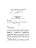
An observation of figure 3.23 learns that the output voltage waveform from
the simulation is aligned with the output obtained from the phasor analysis after
a time interval of approximately 30ms. There is therefore a ‘transient’ effect
present which cannot be ‘seen’ with the phasor analysis. A further observation
of figure 3.23 learns that under steady-state conditions a phase angle error exists
between input and output waveforms which is caused by the presence of the
magnetizing inductance L
m
. It can be shown that the output phasor u
2
may be
The Transformer 67
expressed in terms of the input current phasor i
1
and parameters R
L
and L
m
.
u

2
=
R
L
i
1

1+
R
L
jωL
m

(3.36)
The denominator of equation (3.36) shows that the angle error is equal to:
arctan

R
L
ωL
m

. Hence during the design/manufacture of transformers for this
purpose it is prudent to maximize the L
m
value and limit the size of R
L
.
3.10.2 Tutorial 2
A Caspoc simulation approach to the previous tutorial is considered here.

Build a Caspoc model with the circuit parameters and excitation as defined
in tutorial 1. A Caspoc implementation example for this tutorial is given in
figure 3.24. The results from this model as displayed with the aid of the ‘scope’
GAI
0.2
SCOPE1
i
2
u
2
i
m
@
1
i
1
@
2
1.475
7.375
-1.475
-147.495m
24.153p
-147.495m
Figure 3.24. Caspoc simulation: current transformer model
module (which may be enlarged to show more details), should match those
given in figure 3.23.
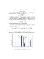
3.10.3 Tutorial 3
A 50Hz, 660V/240V supply transformer is considered in this tutorial. The
object is to determine the parameters of the transformer in question using data

obtained from a no-load and short-circuit test. In the second part of this tu-
torial a Simulink based dynamic model is to be built. This model will then
be used to examine the behaviour of the transformer under load conditions. A
phasor analysis is also required so that the steady-state results obtained with
the Simulink model can be verified. The symbolic model of the transformer, as
given in figure 3.25, is based on the symbolic model discussed in this chapter
(see figure 3.18). The model used in this tutorial is extended by the addition
of a resistance R
M
placed across the terminals of the primary. The power
dissipated in this resistance represents the so-called ‘iron losses’(due to eddy
currents and hysteresis) in the transformer. In a three inductance model, shown
in figure 3.13, this resistance is usually connected in parallel with the inductance
68 FUNDAMENTALS OF ELECTRICAL DRIVES
L
m
. Positioning this resistance across the primary terminals (or the terminals
which correspond to the supply side) simplifies the generic model at the price of
a marginal reduction in accuracy. Under steady-state conditions the power (in
Watts) dissipated in a resistance is given as P
R
= I
2
R = U
2
/R,whereU, I
represent the RMS voltage and current seen by the resistance. The transformer
Figure 3.25. Transformer model with iron losses
was identified at the start of this tutorial by the voltage ratio 660/240, which
represents the rated primary and secondary RMS voltage values of this unit. To

determine the parameters of this transformer a ‘no-load’ test was carried out
where the primary (terminal 1 side) was connected to a 660V, 50Hz sinusoidal
supply source and the secondary side open circuited. The measured current
and power under these conditions were found to be 0.2A(RMS) and 20W re-
spectively. Furthermore, the voltage across the secondary winding was found
to be 240V(RMS). A second ‘short-circuit’ test was also carried out, where the
secondary winding was connected to a 8V(RMS), 50Hz voltage source, which
gives a rated secondary current of 20A(RMS) with the primary winding short-
circuited. Note that in this example the short-circuit test is carried out from the
secondary side (voltage source connected to the secondary winding), which is
often done in case the primary voltage is relatively high, as is the case here.
The secondary power was also measured under these circumstances and found
to be 20W. On the basis of these experimental tests the parameters of the model
according to figure 3.25 can be identified with reasonable accuracy.
The solution to this problem requires a phasor analysis, given that the ex-
perimental data was obtained under ‘steady-state conditions’. Under ‘no-load’
conditions we can simplify the model according to figure 3.25 by assuming that
the voltage drop across the primary resistance and leakage inductanceis small in
relation to the applied primary voltage. The primary current in phasor represen-
tation (under no-load only) is of the form i
1
= i
RM
+ i
LM
,where(i
RM
,i
LM
)

represent the current through components R
M
and L
M
respectively. The RMS
current through the resistance R
M
is found using I
RM
= P
1
/U
1
=20/660,
where P
1
and U
1
represent the measured no-load power and RMS voltage
respectively. The winding ratio k is found using k  U
1
/U
2
. The current
through L
M
is found using I
LM
=


(I
1
)
2
− (I
RM
)
2
,whereI
1
represents the
The Transformer 69
measured (RMS) no-load primary current. Note that I
RM
has already been
calculated. On the basis of these calculations and no-load data the following
parameters are obtained
k 
U
1
U
2
(3.37a)
R
M

(U
1
)
2

P
1
(3.37b)
L
M

U
1
ω

(I
1
)
2
−

P
1
U
1

2
(3.37c)
where U
1
,U
2
,I
1
and P

1
, shown in equation (3.37), represent the no-load
experimental data.
Under short-circuit test conditions the model according to figure 3.25 can be
simplified by ignoring the magnetizing current and iron losses. The reason for
this is that the secondary voltage is very low compared to normal operation.
Hence the current whichflows in R
M
and L
M
is small in comparisonto the rated
primary current. Consequently, the currents which flow in these components
can be ignored when the transformer is exposed to a short-circuit test. For the
calculation linked to this test we will refer to the applied secondary voltage and
measured secondary current to the primary side. Which means that we can con-
sider (for calculation purposes) the short-circuit problem from the primary side.
The total resistance R
p
as seen from the primary side consists of the primary
resistance R
1
to which we must add the primary referred secondary resistance
R

2
= k
2
R
2
. The leakage reactance ωL

σ
completes this series network, which
is excited by a primary referred secondary voltage U

2
= kU
2
. The primary
referred secondary current is equal to I

2
= I
2
/k. The short-circuit impedance
Z
p
as seen from the primary side is equal to Z
p
= U

2
/I

2
=

R
2
p
+(ωL

σ
)
2
.
The impedance Z
p
can therefore be found on the basis of the applied secondary
voltage U
2
, calculated winding ratio k and measured current I
2
. In addition, the
short-circuit power P
2
was measured which may be written as P
2
=(I

2
)
2
R
p
.
From this equation the total resistance as ‘seen’ from the primary side can be
obtained. The individual resistance values cannot be found (unless they are
measured directly with the aid of an Ohm meter) from these measurements and
the assumption made in this case is that R

2

= R
1
. The parameters, which are
obtained from the short-circuit measurements are calculated as follows
R
p
 k
2
P
2
I
2
2
(3.38a)
R
1

R
p
2
(3.38b)