Digital logic testing and simulation phần 4 doc
Bạn đang xem bản rút gọn của tài liệu. Xem và tải ngay bản đầy đủ của tài liệu tại đây (616.37 KB, 70 trang )
THE SUBSCRIPTED D-ALGORITHM
187
resolved by assigning a fixed binary value to the output of gate 8. If a 1 is assigned,
then one of the inputs must be set to 0. However, the other flexible signal can still be
instantiated.
Generally, when an input must be set to a controlling value—for example, a 0 on
an input to an AND or NAND gate—it is usually preferable to choose the input that
is easiest to control. However, in the present case an additional criterion may exist. If
a fault on one of the two inputs to gate 14 has already been detected, then the flexi-
ble signal D
1
or D
2
corresponding to the undetected input fault can be favored when
a choice must be made. When D
1
and D
2
converge at the output of gate 8, if it is
found that the upper input to gate 14 has already been tested, then D
1
can be purged
by assigning a 0 to the upper input of gate 8.
When a conflict occurs, its resolution usually requires that segments of D
i
chains
be deleted. AALG accomplishes this with functions called DROPIT and DRBACK.
8
DROPIT purges a chain segment when the end closest to the primary inputs is
known. It works forward toward the gate under test. It must examine fanouts as it
progresses, so if two converging paths both have flexible signals, then both chain
segments must be deleted. When a flexible signal is deleted, it may be replaced by a
fixed binary signal. This signal, when assigned to the input of a gate, may be a con-
trolling value for that gate and thus implies a logic value on the output. In that case,
the output must be further traced to the input of the gate(s) in its fanout to determine
whether this output value is a controlling value at the input of the gate in its fanout.
When D
0
was assigned to the output of gate 14, a conflict occurred at gate 8, so a 1
was assigned to its output, which required a 0 on one of its inputs. Primary input 6
was chosen. This required that the D
2
chain from P.I. 6 to the input of gate 14 be
purged. A 0 on P.I. 6 implies a 0 on the output of gate 12, so the flexible signal D
2
ini-
tially assigned at the output of gate 12 must be purged and the path traced another
level. At gate 14 the enabling signal 0 is assigned to the lower input and the flexible
signal D
1
is assigned to the upper input. Therefore DROPIT can stop at that point.
If D
j
controls the output and one or more D
i
control the inputs, it may be desir-
able to propagate D
j
toward the inputs and purge the D
i
signals. In that case the end
of the chain farthest from the PIs is known and DRBACK purges the chain. Working
back toward the PIs, it may have to purge a considerable number of flexible signals
since the signals were originally replicated when working toward the inputs.
The functions DROPIT and DRBACK are not always invoked independently of
one another. When DROPIT is purging flexible signals and replacing them with
fixed binary signals, it may be necessary to invoke DRBACK to purge other chain
segments. This is seen in the upper branch of the circuit in Figure 4.10. Primary
input 2 was assigned a 0 because of a conflict. Therefore DROPIT, working for-
ward from primary input 2, purges D
1
and replaces it with a 0. The 0 on the lower
input of gate 9 blocks the gate and therefore DRBACK must pick up the chain seg-
ment on the upper input and delete it back to input 1 and replace it with X. Then
DROPIT regains control and proceeds forward. The 0 on the input of gate 7
implies a 0 on the output and hence a 0 on the input to gate 13. Since a 0 on an OR
gate is not a controlling value, the forward purge can stop, leaving gate 13 with
(0, D
1
) on its inputs.
188
AUTOMATIC TEST PATTERN GENERATION
To help identify and purge unwanted chain segments, flexible signals are never
implied forward to primary outputs during back-propagation. As an example, in
Figure 4.10, when back-propagating from gate 9 toward primary inputs, any assign-
ment to primary input 2 will necessarily imply the inverse signal on the output of
gate 7. However, if the flexible signal is assigned, then at some later point DROPIT
may go unnecessarily along signal paths, deleting flexible signals and replacing
them with controlling logic values where it may be unnecessary.
In measurements of performance, it has been found that AALG creates an input
pattern with flexible signals in about the same time that the D-algorithm generates a
single pattern. Overall time comparison for typical circuits shows that it frequently
processes a circuit in about 30% of the time required by the D-algorithm. AALG is
especially efficient, for reasons explained earlier, when working on circuits that have
gates with large numbers of inputs, as is sometimes the case with programmable
logic arrays (PLAs). The efficiency of AALG can be enhanced by first selecting pri-
mary outputs and then selecting gates with large numbers of inputs. Gates for which
the output has not yet been tested are chosen next since they usually indicate regions
where fault processing has not yet occurred. Finally, scattered faults are processed.
On those faults AALG occasionally defaults to the conventional D-algorithm.
4.6 PODEM
The D-algorithm selects a fault from within a circuit and works outward from that
fault back to primary inputs and forward to primary outputs, propagating, justifying
and implicating logic assignments along the way. In circuits that rely heavily on
reconvergent fanout, such as parity checkers and error detection and correction
(EDAC) circuits, the D-algorithm may encounter a significant number of conflicting
assignments. When that happens it must find a node where an arbitrary choice was
made and choose an alternate assignment. This can be very CPU and/or memory
intensive, depending on how many conflicts occur and how they are handled.
PODEM (path-oriented decision making)
9
reduces the number of remade deci-
sions by selecting a fault and assigning logic values directly at the circuit inputs to
create a test. Much of its efficiency results from its ability to exploit the fact that sig-
nal polarity along sensitized paths is irrelevant. For example, when the D-algorithm
propagates a D or D through an XOR, it assigns a 1 or 0 to the other input, the
choice being arbitrary and often depending on how the software was coded. It may
then go to great lengths to justify that choice, despite the fact that either choice is
equally effective, and the chosen value may eventually produce a conflict, necessi-
tating a remade decision. PODEM, as we shall see, implicitly propagates through
the XOR, eliminating the need to make a choice at the other input, thus obviating the
need to make or alter a decision.
PODEM begins by initializing the circuit to Xs. A fault is chosen, and PODEM
backs up through the logic until it arrives at a primary input, where it assigns a
binary value, 0 or 1. Implications of this assignment are propagated forward. If
either of the following propositions is true, the assignment is rejected.
PODEM
189
1. The net for the selected stuck fault has the same logic value as the stuck fault.
2. There is no signal path from an internal net to a primary output such that the
internal net has value D or D and all other nets on the signal path are at X.
Proposition 1 excludes input combinations that cause the fault-free circuit to assume
the same value as the stuck-at value at the site of the fault. Proposition 2 rejects
input combinations that block all possible paths from the fault to the outputs. If the
test is not complete and if there is no path to an output that is free to be assigned,
then there is no way to propagate a test to an output.
When PODEM makes assignments to primary inputs, it employs a branch-and-
bound method.
10
This process is represented by the tree illustrated in Figure 4.11.
An assignment is made to a primary input and is implied forward. If the assignment
does not violate proposition 1 or 2, it is retained and a branch is added to the tree. If
a violation occurs, the assignment is rejected and the node is flagged to indicate that
one value had been unsuccessfully tried. The tree is thus bounded. If the node had
been previously flagged, then it is completely rejected and it becomes necessary to
back up in the tree until an unflagged node is encountered, at which point the alter-
nate value is implied. The process continues until a successful test is created or the
process returns to the start node and both choices have been tried. If that occurs, it is
concluded that a test does not exist. The criterion for a successful test is the same as
that employed by the D-algorithm, namely, that a D or D has propagated from the
point of a fault to a primary output.
If PODEM rejects the initial assignment to the ith input selected, and if there are n
primary inputs, then 2
n–i
combinations have been eliminated from further consider-
ation. If the initial assignment to the first primary input is rejected, then the number of
Figure 4.11 Branch-and-bound without backtrace.
PI
4
= 1
PI
3
= 0
PI
2
= 1
PI
1
= 1PI
1
= 0
PI
2
= 0
PI
5
= 0
PI
4
= 0
SUCCESS
All PIs initially
set to X
}{
START
190
AUTOMATIC TEST PATTERN GENERATION
combinations to be considered has been cut in half. We say, therefore, that PODEM
examines all input combinations implicitly. It does not have to explicitly evaluate all
assignments in order to determine if a test exists. Since it will consider all possible
input combinations if necessary to find a test, it can be concluded that if PODEM does
not find a test, a test does not exist; hence it follows that PODEM is an algorithm.
PODEM can be implemented by means of a last-in, first-out (LIFO) stack. As
primary inputs are selected, they are placed on the stack. A node is flagged if the
initial assignment was rejected and the alternate choice is being tried. If a node
assignment violates one of the two propositions and the node is flagged, then the
node is popped off the stack, thus bounding the graph. Nodes continue to be popped
off until an unflagged node is encountered. The process terminates when a test is
found or the stack becomes empty.
Example The branch-and-bound method is illustrated in Figure 4.11, correspond-
ing to an SA0 on input 3 of gate K of the circuit in Figure 4.1. In this example, the ini-
tial trial assignments are arbitrarily chosen to be 0. When a 0 is assigned to I
1
a
problem occurs immediately because the output of gate H becomes 0, and that violates
rule 1 above. Therefore the assignment is rejected and the alternate value is assigned.
The initial assignment to I
2
is rejected for the same reason. The assignment I
3
= 0 is
retained, at least for the moment, because it does not violate either of the two rules.
The next assignment, I
4
= 0, has to be rejected because it causes the output of gate C
to become 0, which causes the output of gate H to become 0, again violating rule 1. The
assignment I
4
= 1 does not violate either of the rules, so it is retained. Finally, the assign-
ment I
5
= 0 completes the test.
PODEM uses the branch-and-bound technique, but its performance is improved
substantially by the use of a backtrace feature. The backtrace starts at the gate under
test or at some other gate along the propagation path and determines an initial objec-
tive. The initial objective is a net value and logic value (n, e), e ∈ {0,1}, that satisfy the
value at the net, either helping to propagate a fault from the input to the output of the
faulted gate or helping to extend a sensitized path from the fault origin to an output.
With an initial objective as its starting point, backtrace works back to the primary
inputs. During processing, backtrace may encounter a gate such as an AND where
all inputs must be set to noncontrolling values. If that happens, it processes the
inputs in order, from the most difficult to the least difficult to control. If the
backtrace encounters a gate where it is necessary to set an input to the controlling
state—for example, a 1 on an input to an OR gate—it chooses the input that is
easiest to control to the desired value.
Example Consider again the circuit in Figure 4.1. For the SA0 on input 3 of gate K,
the output of gate F must be 0, so one of its inputs must be 1. If the top input is chosen,
the 1 comes from inverter A, which requires that I
1
be 0. Implying this assignment
causes the output of gate H to become 0. Since gate H drives the third input to K, which
is being tested for a SA0 fault, that input must be a 1. This conflict necessitates that
primary input I
1
be set to 1, which implies a 0 on the output of gate A.
PODEM
191
Since I
1
is set to 1, the top input to K remains unassigned, so another backtrace
must be performed from that input, but values implied by the logic 1 on I
1
must not
be altered. Therefore, the 0 on the output of gate F is justified this time by a 1 on input
I
2
. The second input to K also requires a 0, which is required from gate G. But that
value is satisfied at this point by the 0 at the output of gate A. The third input to K, the
input being tested for a SA0 fault, must be set to 1. A backtrace from that input may
encounter gate B or C, both of which must provide a 1. Assume that gate B is pro-
cessed first. Gate B equals 1 only if one of its inputs is 0, so set I
3
to 0. At this point,
gate C is still at X. To get a 1 from gate C requires another backtrace, which causes
input I
4
to be set to 1.
The sensitized path must now be propagated forward to the output. If the circuit is
rank-ordered and if the rule is to drive the fault to the highest numbered gate, using the
crude metric that the highest numbered gate is closest to an output, then gate N is cho-
sen for propagation. With the sensitized signal on the upper input to gate N, the lower
input to N must be a 1. Since K has the test signal D
, it is necessary to get a 0 from gate
L. The upper input to L has a 0, and I
4
= 1, so the backtrace chooses I
5
to be 0.
The backtrace operation determines which primary inputs are relevant when test-
ing a given fault. Furthermore, the backtrace often, but not always, chooses the cor-
rect value as the initial trial value for the branch-and-bound operation. A smart
backtrace—that is, one that uses clever heuristics—can reduce the number of back-
tracks needed on the primary inputs. This will be seen in Section 4.7, which
discusses the FAN algorithm. The algorithm for PODEM is described below in
pseudo-C-code; that is, it follows the C programming language syntax for loop
control. For example, in C the expression
for(;;) { one or more lines of code }
represents an infinite loop. The only way out is to perform a break somewhere in the
code. The open parentheses and close parentheses ({}) are used in lieu of begin and
end to demark a block of two or more lines of code, and they are used to denote a set
or collection of objects. For example, {primary inputs} denotes a set of primary
inputs. Which primary inputs are being referred to will be evident from the context.
Also, two consecutive equal signs (==) indicate a comparison. Note that the back-
trace routine searches for an X-path. That is a path from the D-frontier to a primary
output which has the value X along its entire length.
PODEM() // call with gate no. and stuck-pin number
{
for(;;) {
status = backtrace(); // returns FAIL or P.I.
if (status == FAIL) { // back up on input
// assignments
for(;;) { // loop through P.I.s
192
AUTOMATIC TEST PATTERN GENERATION
if (decision_stack == EMPTY)
return(FAIL); //no more P.I.s,
//undetectable fault
else if (decision_stack.flag == 0) { //try alt.
value
P.I.[j] = - P.I.[j]; //complement the
//assignment
decision_stack.flag = 1;
break;
}
else { // back up
P.I.[j] = X;
decision_stack.flag = 0;
pop decision_stack;
}
}
}
//either fall-through or come here after
//returning from backtrace(), i.e., status == P.I.
imply P.I.s;
if (TEST == success) //D or DBAR reached P.O.
return (TEST); //return with test vector
}
}
backtrace() //initial objective
{
if (G.U.T. output != X) { //gate under test
for(;;) { //loop through D-frontier
choose gate B in D-frontier closest to an output;
if (gate == NULL) //either D-frontier is empty,
return(FAIL); //or no X-path to an output
//exists
else if (X-path exists from B to output){
//propagate
set output of B to 1(0) if AND/NOR(NAND/OR);
break;
}
else continue; //check next entry in D-frontier
}
}
else { //output of G.U.T. is X
FAN
193
if (stuck fault is on G.U.T. input pin) {
if (faulted input == X)
faulted input = -(stuck-fault direction);
else //propagate value
set G.U.T. output to 1(0) if G.U.T. is AND/NOR
(NAND/OR);
}
else
G.U.T. output = -(stuck-fault value); // complement
}
for(;;) { //work back until a P.I. is reached
if (objective net driven by P.I.[j])
return(P.I.[j]); //reached a P.I.
else { //objective net is driven by gate Q
if ((OR/NAND and C_O == 1) or (AND/NOR and C_O == 0))
choose new objective net n; //input to Q
// n = X, and EASIEST to control
else
// ((OR/NAND and C_O == 0) or (AND/NOR and C_O == 1))
choose new objective net n; //input to Q
// n = X, and HARDEST to control
}
if (Q == NAND/NOR) //complement the current
//objective level
objective level = -(C_O logic level);
else //Q is AND/OR
objective level = C_O logic level;
}
}
4.7 FAN
FAN
11
(fanout-oriented test generation algorithm), like PODEM, uses implicit enu-
meration. However, it employs a number of additional features designed both to
reduce the number of backtracks and to minimize the amount of processing during
each backtrack. Some of the more significant enhancements include:
● Maximum use of implication, forward and back
● Multiple backtrace
194
AUTOMATIC TEST PATTERN GENERATION
● Unique sensitization
● Stop at head lines
● Seek consistency at fanout points
PODEM assigns binary values to primary inputs and implies them forward. By
way of contrast, FAN implies assignments in both directions to the fullest extent
possible in order to more quickly detect conflicts. Consider the circuit in Figure 4.1.
Suppose the bottom input of gate G is SA1. The PDCF is (1,1, 0, 0) (note that the
bubble on input 3 represents a signal inversion). When all implications, forward and
back, of that PDCF are carried out, the fault is immediately seen to be undetectable.
However, PODEM may perform several computations, even on this small circuit,
before it concludes that the fault is undetectable. These faults cause ATPG programs
to expend a lot of useless computational effort because many possibilities frequently
must be explored before it can be concluded that the fault is undetectable. If a circuit
has many undetectable faults, the ATPG may expend half or more of its CPU time
attempting to create tests for these faults. Efficient operation of an ATPG dictates
that undetectable faults be found as quickly as possible.
The multiple backtrace enables FAN to reduce the number of backtraces and
more quickly identify conflicts. Consider again the circuit in Figure 4.1. When justi-
fying a 1 on the third input of gate K, PODEM used two backtraces: The first back-
trace set I
3
to 0, and the second backtrace set I
4
to 1. When FAN is backtracing, it
recognizes that a 1 on the output of gate H requires that all of its inputs be at 1, so
those values are immediately assigned to its inputs. Any assignment that conflicts
with those assignments is immediately recognized. In addition, the backtrace from
the third input of K to the inputs of H are avoided.
The PODEM algorithm, as published, chooses the input that is most difficult to con-
trol if all inputs must be assigned noncontrolling values. The reason for choosing the
most difficult assignment is that if there is a problem, or conflict, that choice is usually
most likely to reveal the conflict as quickly as possible. However, PODEM only assigns
the input that is most difficult to control. Thus, if a three-input AND gate requires 1s on
all inputs, and all inputs are driven by primary inputs, PODEM will backtrace three
times. The multiple backtrace assigns 1s to all three inputs immediately.
The unique sensitization operation is performed whenever the D-frontier consists of
a single gate. Consider the circuit in Figure 4.12. AND gate G is being tested for a SA1
fault on its upper input. The fault must propagate through the multiplexer and then
through AND gate H. In order for the fault effect to get through gate H, its upper input
must be 1. But, when setting up the PDCF, it is possible that the upper input to H was
set to its blocking value. A lot of unnecessary computations might be performed before
that conflict is revealed. FAN searches forward along the propagation path to an output
searching for these situations. Note that the fault propagates through the select line of
the mux, which enters reconvergent logic, so nothing can be said about the logic inside
that function. When a situation such as that which exists at gate H is encountered, the
nonblocking value, in this case the logic value 1, is implicated back toward the primary
inputs. The values on the primary inputs must establish a 0 on the faulted input to G,
and at the same time they must establish a 1 on the upper input of H.
FAN
195
Figure 4.12 Unique sensitization.
Backtracing in FAN is aided by the observation that fanout-free regions (FFRs)
usually exist in the circuit being tested. FFRs are single-output subcircuits that do
not contain reconvergent logic; hence they can be justified without concern for
conflicts. As a result, a backtrace can stop at the outputs of the FFRs. After all
other assignments have been made, justification of the FFRs can be performed.
This can be seen in the circuit in Figure 4.13, which will be used to help define
some terminology.
When a net drives two or more gates, the part of the net common to every branch
is called a fanout point. In Figure 4.13 the segment J, which is common to J
1
and J
2
,
is a fanout point. (In this circuit, except for fanout branches, nets will be identified
with the gates that drive them.) If a path exists from a fanout point forward to a net
P, then P is said to be bound. A net that is not bound is free. In Figure 4.14 the nets
A, B, C, D, E, F, G, H, I, and J are free nets, and the nets J
1
, J
2
, K, and L are bound
nets. Note that the net connecting the output of gate J to gates K and L has three
identifiable segments: segment J, which is the fanout point; segment J
1
, which
drives gate K; and segment J
2
, which drives gate L. Free nets that drive bound nets,
either directly, as in the case of the fanout point J, or through a logic gate, as in the
case of K, are called head lines; they define a boundary between free lines and
bound lines.
The FAN algorithm works with objectives. These are logic assignments that must
be satisfied during the search for a test solution. A backtrace in FAN begins with ini-
tial objectives. At the start of the algorithm initial objectives are determined by the
Figure 4.13 Identifying head lines.
Z
A
MUX
B
C
D
E
Sel
F
G
H
A
B
E
F
H
K
G
C
D
L
J
2
J
1
J
head lines
I
J
}
196
AUTOMATIC TEST PATTERN GENERATION
Figure 4.14 Identifying/resolving a conflict.
PDCF. The initial objectives become current objectives upon entering the routine,
denoted Mback, that performs the multiple backtrace. During the backtrace, logic
assignments are made in response to current objectives. These assignments become
new current objectives, or they may become head objectives or fanout point objec-
tives, which must eventually be satisfied. Objectives that occur at head lines are
called head objectives. Objectives at fanout points are called fanout point objectives
(FPOs).
While assigning logic values to justify current objectives during backtrace, FAN
stops at fanout points and head lines until all current objectives have been satisfied.
Then the backtrace selects an FPO closest to the primary output, if one exists. Head
objectives are always satisfied last, after all other objectives have been satisfied,
since there is no reconvergent fanout and they can be satisfied without fear of con-
flict. If the FPO has conflicting requirements, the conflict must be resolved. A con-
flict occurs if, during the multiple backtrace, two or more paths converge on the
fanout point with different requirements. If the FPO does not require conflicting
assignments, the MBack routine continues from this FPO.
In order to maintain a record of logic values that must be assigned during back-
trace, as well as to recognize conflicts, FAN employs an objective expressed as a trip-
let (s, n
0
(s), n
1
(s)). In this triplet, s denotes the objective net, n
0
(s) is the number of
times a 0 is required at s during the backtrace, and n
1
(s) is the number of times a 1 is
required at s. A conflict exists if both n
0
(A
i
) and n
1
(A
i
) are nonzero. If a conflict exists,
the rule is: If n
0
(A) < n
1
(A), assign a 1 to the fanout point, otherwise assign a 0.
Logic values assigned during backtrace depend on (a) the function of the logic
gate through which the backtrace passes and (b) the value required at the output of
that gate. For an AND/NAND gate, a 1/0 on the output requires 1s on all inputs. For
an OR/NOR gate, a 0/1 on the output requires 0s on all inputs. In addition, if the out-
put is complemented, then the values n
0
and n
1
are reversed in the triplet. For exam-
ple, given a NOR gate with triplet (Z, u, v) at its output, the triplet assigned to each
of its inputs X
i
is (X
i
, v, u) if a 1 is needed at the output.
N
M
G
K
L
H
J
1
0
1
1
1
0
(R,0,1)
P
0
B
A
D
C (C,0,3)
F
E
U
T
(K,3,0)
(P,0,2)
(Q,0,2)
(U,1,0)
(T,1,0)
(S,2,0)
S
(N,0,1)
(M,0,3)
(G,2,3)
(L,0,2)
(H,0,3)
(J,2,0)
(B,3,2)
(A,0,2)
(D,0,0)
R
Q
FAN
197
If a controlling value is required on the input of a gate (0 on an AND or NAND
gate, 1 on an OR or NOR gate), then the backtrace is made through the input that is
easiest to control. Assume a logic gate with inputs X
1
, X
n
, and output Y, and, with-
out loss of generality, assume that input X
1
is the easiest input to control. Then Table
4.1 contains the criteria used to compute the values n
0
and n
1
at each input net.
Consider the AND gate: If a 0 is required at its output, then a 0 must be applied to
one of its inputs. Assign a 0 to the input that is easiest to control, unless that input
has already been tried and rejected. The values n
0
(X
1
) and n
1
(X
1
) at that input are
equal to the value at the output. For noncontrolling inputs we have n
0
(X
i
) = 0 and
n
1
(X
i
) = n
1
(Y). Similar considerations hold for the NAND gate except that from
Table 4.1 it can be seen that the subscripts are reversed. The analysis for the OR and
NOR gates are similar, but complementary.
At FPOs the values n
0
and n
1
are summed. This is in recognition of the fact that,
during backtrace, two or more paths driven by that FPO may have requirements to
justify signals further along toward the output. Furthermore, if two or more nets
require the same value from an FPO, by summing their requirements, it is possible
to determine how many signal paths depend on each value, 0 or 1, generated by
that FPO.
These computations can be illustrated using the circuit in Figure 4.13. Assume
the values (J
1
,1,1) and (J
2
,1,2) occur at segments J
1
and J
2
during backtrace in order
to justify assignments made closer to the output. The value 0 has weight 2, and the
value 1 has weight 3. When this happens, the logic value 1 is chosen to be assigned
at the FPO. But, since that represents a conflict, the multiple backtrace is halted at
this point and conflict resolution is performed. That involves backtracking on
assignments made to the FPO and trying alternate assignments. If a self-consistent
set of assignments to the FPOs cannot be found, the fault is undetectable.
TABLE 4.1 Assignment Criteria
Function 0-count 1-count Controllability
1 AND n
0
(X
1
) = n
0
(Y) n
1
(X
1
) = n
1
(Y) Easiest 0
2 AND n
0
(X
i
) = 0 n
1
(X
i
) = n
1
(Y) Others
3 NAND n
0
(X
1
) = n
1
(Y) n
1
(X
1
) = n
0
(Y) Easiest 0
4 NAND n
0
(X
i
) = 0 n
1
(X
i
) = n
0
(Y) Others
5OR n
0
(X
1
) = n
0
(Y) n
1
(X
1
) = n
1
(Y) Easiest 1
6OR n
0
(X
i
) = n
0
(Y) n
1
(X
i
) = 0 Others
7 NOR n
0
(X
1
) = n
1
(Y) n
1
(X
1
) = n
0
(Y) Easiest 1
8 NOR n
0
(X
i
) = n
1
(Y) n
1
(X
i
) = 0 Others
9NOT n
0
(X) = n
1
(Y) n
1
(X) = n
0
(Y)
10 Fanout
n
0
X() n
0
X
i
()
i 1=
k
∑
= n
1
X() n
1
X
i
()
i 1=
k
∑
=
198
AUTOMATIC TEST PATTERN GENERATION
Example The circuit in Figure 4.14 will be used to illustrate the operation of FAN.
In this circuit, inputs A and B are primary inputs, while C, D, E, and F are inputs from
other parts of the circuit and, where choices must be made, we will assume that C, D,
E, and F are the more difficult choices. Calculations are summarized in Table 4.2. The
example starts with objectives at the nets R, T, and U. The values on nets T and U are
summed to give the value (S,2,0) at net S. Likewise, the triplets at N and P are summed
to yield the triplet (M,0,3). This requires a 0 on one of the inputs to M and, for sake of
illustration, we assume that net K is the easiest to control. Because M is a NAND, the
values n
0
and n
1
of the triplet at K are reversed. Eventually, the fanout point G is
reached, but with conflicting requirements. Since segment H has a higher weight, a 1 is
assigned to fanout point G. Since G is a headline, assignments to A and B are postponed.
Because G has conflicting requirements, the function MBack is exited and FAN
implies the value 1 that was assigned to G. The assignment conflicts with the require-
ment at L. That requirement comes from net Q, whose objective is (Q,0,2). But that
objective might be satisfied by the unidentified logic driven by net F, in which case the
conflict at G is resolved. If, however, the conflict cannot be resolved, the alternate
value, 0, is assigned to G. The conflict along that path can be resolved by assigning a 0
to net D. All affected triplets must then be recomputed. Then MBack selects an FPO
from which it backtraces in order to obtain and satisfy new current objectives.
We leave it to the reader to complete this example. The FAN algorithm is
described in pseudo-C-code at the end of this section.
The first step in FAN is to assign a PDCF for the fault. Then, a backtrace flag is
set. The flag enables MBack to distinguish between those instances where a back-
trace starts from a set of initial objectives (IO), entry A, or from a set of fanout point
objectives (FPO), entry B. Entry B to the backtrace routine is entered in order to
continue a multiple backtrace that terminated at a fanout point.
TABLE 4.2 Keeping Track of Objectives
Current Objectives Stem Obj. Head Obj.
(R,0,1), (T,1,0), (U,1,0)
(T,1,0), (U,1,0), (N,0,1)
(U,1,0), (N,0,1) (S,1,0)
(N,0,1) (S,2,0)
(S,2,0), (M,0,1)
(P,0,2), (Q,0,2) (M,0,1)
(Q,0,2) (M,0,3)
(L,0,2) (M,0,3)
(J,2,0) (M,0,3)
(G,2,0)
(K,3,0) (G,2,0)
(H,0,3) (G,2,0)
(G,2,3)
(F,0,2) (G,2,3)
FAN
199
A sensitized value, D or D, results either from a stuck-fault on the output of a
gate, or from a stuck-fault on the input of the gate, in which case it is implied to the
output of the gate. The sensitized value continues to be propagated forward from
there. If the output of the faulted gate only drives a single destination gate, then the
sensitized signal can be propagated to the output of that gate, with the result that
additional nonblocking assignments on the input of that gate are added to the set of
initial objectives. If the D-frontier consists of two or more entries, FAN examines
the entries in the D-frontier to ensure that they are all legitimate; that is, they all
propagate to output pins and are not blocked. Then FAN orders these paths in terms
of ease or difficulty of propagation. However, like the D-algorithm, an implementa-
tion in FAN must, if necessary, eventually consider all single and multiple propaga-
tion paths at FPOs to truly be considered an algorithm.
The MBack routine has two entries. At entry A the initial objectives become the
set of current objectives {CO}. If {CO} is non-empty, then an objective is selected.
While MBack traces back through the circuit, if it encounters a head line, that head
line is added to the set of head objectives {HO}. If it encounters a logic gate, then it
must be determined if the gate requires a controlling or noncontrolling value on its
inputs. As previously discussed, the rules in Table 4.1 are used to select an input and
a value to be assigned to that input. The net driving the input is added to the set of
current objectives. If the net is a fanout branch, then n
0
and n
1
are updated. However,
fanout points are not processed until all of the nonfanout gates are justified.
The other entry to MBack is entry B. This entry is used if the set of current objec-
tives is empty, then an FPO is selected from the set {FPO}. If there is no conflict,
MBack continues from the FPO. However, if the node has conflicting requirements,
then the conflict has to be resolved. This is accomplished by means of a backtrack
through the FPO assignments.
Initially the backtrace flag is on if there are unjustified nets at the completion of the
implication stage. At this point all sets of objectives are initialized to empty (EMPTY)
and the backtrace flag is reset. If there are unjustified lines, they become the set of ini-
tial objectives {IO}. If the error signal did not reach a primary output, a gate in the D-
frontier is added to {IO}. A multiple backtrace is then performed by the MBack func-
tion. If the backtrace flag is not on, then there are no nets waiting for logic assign-
ments. In that case, the set of fanout point objectives {FPO} are examined. If the set
is nonempty, then a multiple backtrace is performed from a selected FPO. At the
completion of the multiple backtrace, if there are no conflicts at any fanout points,
then the set of header objectives {HO} are processed. If there is a conflict at a fanout
point—that is, both n
0
( f ) and n
1
( f ) are nonzero—then the value assigned is based on
which value is larger. Since both values are nonzero, there is obviously a conflict that
must be resolved. Looking again at the final_objective function, a value is assigned
and a return is made to the implication step, where a conflict leads to block 8.
FAN() //call with gate no. and stuck-pin number
{
assign PDCF; //primitive D-cube of
//failure
200
AUTOMATIC TEST PATTERN GENERATION
backtrace_flag = A; //backtrace from
//unjustified lines
for(;;) //loop forever
{
implicate assignments; //forward and back
if (backtrace unnecessary)
backtrace_flag = B; //process FPO
if (fault signal reached a P.O.) {
if (# unjustified bound lines == 0) {
justify free lines; //done
return (TEST);
}
else {
final_objective();
assign value to final objective line;
}
}
else {
if (# gates in D-frontier > 1) { //choose gate
//closest to P.O.
final_objective();
assign value to final objective line;
}
else if (# gates in D-frontier == 1)
unique sensitization;
else { //no. gates == 0
if (there are untried combinations) {
set untried combination;
backtrace_flag = B;
}
else
return (FAIL);
}
}
}
}
final_objective()
{
mb = 0;
if (backtrace_flag == A)
mb = MBack(A);
FAN
201
else if (fanout objectives != EMPTY)
mb = MBack(B);
if (mb == D) { //MBack() returns with ‘C’ or ‘D’
final_objective = FPO;
return;
}
for (;;)
{
if (head_objectives == EMPTY)
mb = MBack(A);
choose Head Objective;
if (headline unspecified)
break;
}
Head Objective = Final Objective;
}
MBack(flag)
{
if (flag == A) {
backtrace_flag = 0;
if (# unjustified_lines > 0)
{initial_objective} = unjustified lines;
if(fault signal did not reach P.O.)
add gate in D-frontier to initial objectives;
{current_objective} = {initial_objective};
if ({current_objective} != EMPTY) {
choose current_objective;
next_obj();
}
else {
if (FPO == EMPTY)
return(C);
else
flag = B; //force execution of the “flag == B”
//code
}
}
if (flag == B) {
choose FPO p closest to P.O.;
if ((p reachable from fault line) or ((n0 == 0) or
(n1 == 0)))
202
AUTOMATIC TEST PATTERN GENERATION
next_obj();
else
return(D);
}
}
next_obj() //next objective
{
if (current_objective == headline)
add current_objective to head_objectives;
else if (current_objective driven by FPO)
add n0 and n1 to FPO //(Table 4.1, rule #10);
else //determine next objectives
backup through gates using Table 4.1 rules #1-9;
//add them to the set of current objectives
}
4.8 SOCRATES
FAN started with PODEM and added enhancements whose purpose was to elimi-
nate unnecessary backtracks and reduce the amount of processing time between
backtracks. In like manner, Socrates
12
started with FAN and identified enhance-
ments that were able to realize further performance gains. Socrates identified
improvements in the implication, unique sensitization, and multiple backtrace pro-
cedures. In addition, Socrates added support for complex primitives such as adders,
multiplexers, encoders, and decoders, as well as XOR and XNOR gates with an
arbitrary number of inputs.
Consider first the implication operation. In Figure 4.15(a) the signal on input A is
a 1. That value passes through both OR gates, implying 1s on the outputs of both OR
gates, thus implying a 1 on the output of the AND gate. Now consider the situation
in Figure 4.15(b). The output of the AND gate is a 0, which implies that input A
must be a 0. This follows from the logic identity (A ⇒ D) ⇔ (~D⇒ ~A), known as
the contrapositive, where the tilde (~) is used to denote the complement. The value
of this observation lies in the fact that if a 0 is assigned to the output of the AND
gate during a backtrace, input A must be assigned a 0; it cannot be treated as a deci-
sion and postponed until later. This, in turn, can lead to earlier recognition of con-
flicts and reduce the number of backtracks.
To recognize these situations, a learning phase is performed prior to entering the
test generation phase. During this learning phase, a 0 is applied to net n
i
and implied.
The result is then analyzed. This is repeated using the value 1. Assume that, during
the implication, n
i
is initialized to the value v
i
, v
i
∈ {0,1}, and net n
j
receives the value
v
j
, v
j
∈ {0,1} as a result of the implication, that is, (value(n
i
) = v
i
) ⇒ (value(n
j
) = v
j
).
Let n
j
be driven by gate g. Thus if (1) v
j
requires all inputs of g to have noncontrolling
SOCRATES
203
Figure 4.15 Implications.
values and (2) a forward implication has contributed to the assignment v
j
to net n
j
,
then the implication (value(n
j
) = v
j
) ⇒ (value(n
i
) = v
i
) is worth learning. Condition 1
is satisfied if v
j
is 1(0) and g is an AND/NOR (OR/NAND) gate, or if g is an XOR or
XNOR gate. An additional function, check_path(n
j
, n
i
), checks the network to
ensure that there is no directed path from n
j
to n
i
. If the circuit is combinational and
rank-ordered and if j > i, check_path() returns the value 0.This ensures that condi-
tion 2 has been satisfied.
It is possible that the procedure just described will not find an implication where
an implication exists; that is, the procedure is a sufficient, but not necessary, condi-
tion to establish than an implication cannot be performed by the implication proce-
dure. However, the payback from the process, in general, outweighs the cost of
performing the learning operation.
The unique sensitization in FAN handles situations in which the D-frontier con-
sists of a single gate and all paths from the D-frontier to the primary output pass
through that gate. Like improved implication, the unique sensitization is accom-
plished by means of circuit preprocessing.
Definition 4.1 A signal y is said to dominate signal x, y ∈ dom(x), if all directed
paths from x to the primary outputs of the circuit pass through y.
Let x be the only signal in the D-frontier. Let the set of signals dom(x) = {y
1
, y
2
,
, y
n
} be the output signals of their corresponding gates in the set G = {g
1
, g
2
, , g
n
}.
Then, for all gates g ∈ G, the noncontrolling value is assigned to all those inputs of
g that cannot be reached from x on any signal path. This is illustrated in Figure 4.16.
The output of gate a has a D assigned. The signal diverges at gates b and c and then
reconverges at inputs e and f of gate g. In this situation the signal d must be set to 1,
the noncontrolling value.
Figure 4.16 Improved unique sensitization.
(a) (b)
B
C
A
1
D
B
C
A
0
D
c
d
a
b
D
e
f
g
204
AUTOMATIC TEST PATTERN GENERATION
Figure 4.17 Uniquely sensitizing multiple paths.
Definition 4.2 A signal y is said to be the immediate dominator of signal x if y ∈
dom(x), and y is the element of dom(x), that has the lowest circuit level.
In this definition, the level of an element in a combinational circuit is determined
by rank-ordering the circuit elements (cf. Section 2.6). If the immediate dominators
of all signals are known, the dominators of any signal x can be determined recur-
sively. For example, if signal y is an immediate dominator signal x, and signal z is an
immediate dominator of signal y, then signal z is a dominator of signal x.
An additional rule for unique sensitization is required in order to handle the sit-
uation depicted in Figure 4.17. Assume that signal a is the only signal in the D-
frontier, or a dominator of the only signal in the D-frontier. It branches out to
three AND gates, all of which have an input from signal b. In addition, one of the
AND gates has a third input c. Assume signal a is the only signal in the D-
frontier, or a dominator of the only signal in the D-frontier, and it branches out to
gates g
1
, g
2
, , g
n
, all of which require the same noncontrolling value 0 or 1. If
signal b branches out to all the same gates g
1
, g
2
, , g
n
, then b is assigned the
noncontrolling value.
The multiple backtrace in Socrates takes advantage of the fact that some com-
monly occurring circuit configurations are processed as primitives. For example,
the gates M, N, O, and P in Figure 4.1 constitute an XOR. If the diagram is altered
so that gates K and L drive an XOR, the circuit function remains unchanged but
three fanout branches are eliminated. An important point to bear in mind about the
XOR is that a sensitized path on one input of a two-input XOR is propagated to its
output regardless of the binary value on the other input. For example, the values
(D,0) produce a D on the output, and (D,1) produce a D
on the output. Therefore,
when propagating through an XOR or XNOR, it is only necessary to ensure that
the other input has a known value and that both inputs do not have sensitized val-
ues. This line of reasoning can be extended to n-input XOR gates, which Socrates
supports.
PODEM was not adversely affected by the XOR because it did not attempt to jus-
tify assignments on the inputs of XOR gates—in contrast to the D-algorithm, which,
particularly in parity trees, can thrash about trying to find a self-consistent set of
assignments to the circuit, making and changing assignments to resolve conflicts.
However, representing the XOR as a primitive simplifies test generation because it
a
c
b
f
e
d
x
D
D
D
1
THE CRITICAL PATH
205
can be recognized as such, whereas representing it as a collection of lower-level
gates doesn’t solve the problem that caused the D-algorithm to thrash about and
simply introduces more fanout points, which introduce additional processing.
Socrates uses Table 4.3, analogous to Table 4.1, to compute the objective triplets
when an XOR is encountered:
In this table, c
ij
represents the controllability cost for setting x
1
to i and x
2
to j, for
i, j ∈ {0,1}, where x
1
and x
2
are the inputs to the two-input XOR and y is the output.
Other, higher-level primitives require similar specific formulas. The main advantage
of higher-level primitives is the reduction of fanout branches. But it is sometimes
possible to realize opportunities not readily inferred from the gate level model. For
example, if a two-input multiplexer has 1s on both data inputs, the output is going to
be 1, even if the select line has an X.
4.9 THE CRITICAL PATH
The D-algorithm starts at a fault origin and works outward from there, stretching the
sensitized path toward outputs and inputs. PODEM selects a fault and attempts to
sensitize a path by working from the primary inputs. FAN adopts features from both
the D-algorithm and PODEM. The critical path
13
starts at primary outputs and
works back toward primary inputs. It has been implemented commercially as
LASAR (logic automated stimulus and response)
14
and was the ATPG companion to
the LASAR deductive fault simulator mentioned in the summary to Chapter 3. It
enjoyed considerable commercial success for several years, having been marketed
by several companies. Like the simulator, the ATPG only recognizes the NAND
gate. This not only simplified deductive fault simulation computations, but also sim-
plified computations for ATPG. In order for critical path to process circuits imple-
mented with other logic primitives, those primitives must be remodeled in terms of
the NAND gate (cf. Figure 4.18).
Processing rules for a circuit being processed by critical path are defined in terms
of forcing values and critical values as they apply to the NAND gate. The forcing
rules for an n-input NAND gate are as follows:
1. If the output of a NAND gate is 0, then the inputs are all forced to 1.
2. If the inputs are all 1, the output is forced to 0.
3. If the output is 1 and all inputs except input i are 1, then input i is forced to 0.
TABLE 4.3 Multiple Backtrace for Two-Input XOR
Formula Condition
n
0
(x
1
) = n
0
(y) n
0
(x
2
) = n
0
(y) c
00
< c
11
n
1
(x
1
) = n
0
(y) n
1
(x
2
) = n
0
(y) c
00
≥ c
11
n
0
(x
1
) = n
0
(x
1
) + n
1
(y) n
1
(x
2
) = n
1
(x
2
) + n
1
(y) c
01
< c
10
n
1
(x
1
) = n
1
(x
1
) + n
1
(y) n
0
(x
2
) = n
0
(x
2
) + n
1
(y) c
01
≥ c
10
206
AUTOMATIC TEST PATTERN GENERATION
Figure 4.18 Some simple transformations.
A value on a node is critical if its existence is required to establish a test. The
rules are as follows:
1. If the output of a NAND gate is a 0, and it is critical, then the inputs are all
critical 1s.
2. If the output is a critical 1 and if all inputs except input i are 1s, then input i is
a critical 0.
If a NAND gate has a critical 0 on its input, then the other input assignments are all
necessary 1s; that is, it is necessary that they be 1s in order for input i to be critical.
In order for a NAND gate to provide a necessary 1 on its output, at least one of its
inputs must have a 0 assigned. That input is always arbitrary or noncritical.
The creation of a test starts with the selection of an output pin and assignment of a
0 or 1 state to that pin. From that pin an attempt is made to extend critical values as far
back as possible toward the inputs using the rules for establishing critical values. Then,
after the path is extended as far back as possible, the necessary states are established.
When complete, a critical path extends from an output pin back to either some internal
net(s) or to one or more input pins (or both). The critical paths define a series of nets or
signal paths along which any gate input or output will, if it fails, cause the selected out-
put to change from a correct to an incorrect value. Since the establishment of a 0 on an
output pin requires 1s on all the inputs to the NAND gate connected to that output, it is
possible to have several critical paths converging on an output pin.
Upon successful creation of a test, the next test begins by permuting the critical 0
on the lowest-level NAND gate that has one or more inputs not yet tested—that is,
the critical 0 closest to the primary inputs. The 0 is assigned to one of the other
inputs to that NAND gate and the input that was 0 is now assigned the value 1. The
test process then backs up again from the critical 0 to primary inputs, attempting to
satisfy these new assignments. A successful test at any level may result in a critical 0
at a lower level becoming a candidate for permutation before another critical 0 on
the NAND gate that was just processed. However, once selected, a NAND gate will
be completely processed before another one is selected closer to the output. Eventu-
ally, after all the inputs to the gate driving the output have been permuted, the output
pin is then complemented, if the complement value hasn’t already been processed,
and the process is repeated.
(a) 3-input OR (b) Exclusive-OR
THE CRITICAL PATH
207
Figure 4.19 Critical assignments.
The practice of postponing necessary assignments until the critical path(s) have
been extended as far back as possible can help to minimize the number of conflicts
that occur. Figure 4.19 illustrates a situation where a net fans out to two NAND
gates (gate 3 is actually an inverter). Assuming that the outputs of gates 2 and 3 are
both critical, if the upper input of gate 2 is established as far back as possible, and
the necessary 1 on the lower input to gate 2 is extended, the assignments on gate 2
will later have to be reversed in order to get a 0 on the input to gate 3. Since the 1 on
the output of gate 3 is critical, by the rules for critical assignments, the input to gate
3 is also critical; hence it will be processed before the necessary 1 on the input to
gate 2. This avoids having to undo some assignments.
Conflicts can occur despite postponement of necessary assignments. When this
occurs, the rule is to permute the lowest arbitrary assignment that will affect the con-
flict. This is continued until a self-consistent set of assignments is achieved. These
concepts will be illustrated using the circuit of Figure 4.20.
Example The first step is to assign a 0 to the output F, which implies 1s on all the
inputs to gate number 8. Then gate 5 is selected in an attempt to extend the critical
path through one of its inputs. That requires inputs 1, 2, 3 = (0,1,1). Hence, input 1 is
critical and inputs 2 and 3 are necessary. We must then get a 1 on the output of gate
6. We try to extend another critical path. Since the middle input of gate 6 is the com-
plement of the value on input 3, a second critical path cannot be extended back
through gate 6 without disturbing the critical path already set up through gate 5. How-
ever, the values already assigned on 1,2, and 3 do satisfy the critical 1 value needed
at the output of gate 6.
We then try to extend the critical path through gate 7. This also fails. Worse, still,
the values already assigned to the inputs are in conflict with the critical 1 assigned to
Figure 4.20 Creating a critical path.
2
3
0
1
0
1
1
2
3
1
1
2
3
4
5
6
7
9
8
F
208
AUTOMATIC TEST PATTERN GENERATION
the output of gate 7 because they force gate 7 to produce a logic 0. We go back to
gate 5 and permute the assignments on its inputs. A critical 0 is assigned to the mid-
dle input and we now have an assignment (1, 2, 3) = (1, 0, 1) that produces 1s on the
outputs of 5, 6, and 7. A critical path now exists from input 2, through gates 5 and 8,
to the output F. Critical paths also exist from the outputs of gates 6 and 7 to the out-
put F.
4.10 CRITICAL PATH TRACING
The purpose of critical path tracing (CPT) is to estimate the fault coverage provided
by a test program.
15,16
CPT performs a logic simulation on a circuit and then, based
on simulation results, it identifies gates with sensitive values, where gate input i is
sensitive if complementing the value of i changes the value of the gate output. Sensi-
tive inputs can be identified on the basis of the dominant logic value (DLV). A DLV
at a gate input is one that forces an output to a value, regardless of the values on the
other inputs. For example, the DLV for AND and NAND gates is 0, while the DLV
for OR and NOR gates is 1. Note that, unlike the previous subsection where critical
path ATPG required all gates to be NANDs, CPT recognizes critical values for ORs,
NORs, and ANDs, in addition to NANDs. The following statements hold for DLVs:
1. If only one input i has a DLV, then i is sensitive.
2. If all inputs have the complement of the DLV, then all inputs are sensitive.
3. If neither 1 or 2 holds, then no input is sensitive.
A net n is said to have critical value v ∈ {0,1} in a test T if T detects the fault n
SAv. CPT involves tracing from POs, which are critical (assuming they have a
known value) and backtracing along sensitive paths to create critical paths. The
critical paths identify detectable faults. In the circuit in Figure 4.21 the dots denote
inputs that are sensitive. The bold lines indicate a critical path. At gate G, both of the
inputs are DLVs, so neither of them is sensitive and the backtrace stops there. Faults
along the critical path can all be declared detected.
Figure 4.21 Tracing the critical path.
A
B
E
F
I
H
G
J
L
C
D
M
1
1
0
1
0
1
1
1
0
0
1
K
0
1
Y
Z
CRITICAL PATH TRACING
209
Ignore for the moment the output Y and consider just the cone feeding output Z.
At gate M both input values are DLVs, so neither input is sensitive. But inspection of
the circuit suggests that an SA0 on the stem emanating from gate I is detectable at
output Z. A concurrent fault simulation of the circuit would show that if the stem
were SA0, then the outputs of both J and K would be 1; hence the output of M would
be 1 in the presence of the fault and would be detected. Interestingly, if logic simula-
tion produced a 0 on the output of I, then both inputs to M would be 1; that is, both
inputs would have DLVs, and CPT would detect the fault.
CPT preprocesses a circuit to identify its cones, which are then represented as an
interconnection of FFRs. After a logic simulation has been performed and sensitive
inputs have been marked, CPT backtraces, from a primary output. As it backtraces,
it identifies critical paths inside fanout-free regions (FFRs) contained in the cone,
where an FFR is a cone (cf. Section 3.6.2) that has no reconvergent fanout. The
inputs to a FFR are fanout branches (FOB) and primary inputs without FOBs. If a
stem is encountered during backtrace through a FFR, it is checked to determine if it
is critical. If it is critical, then critical path tracing continues from that stem.
If circuits did not contain reconvergent fanout, CPT would be straightforward.
However, reconvergence is an attribute of just about all digital circuits, and one of
the consequences of reconvergence is self-masking, in which a fault effect (FE)
propagates along two or more paths and reconverges with opposite parities or
polarities at a gate, where the FEs cancel out. As an example, if gate K in
Figure 4.21 were a buffer, rather than an inverter, then the lower input to M would
be sensitized. A fault at the stem emanating from I could reach the sensitized
input through the buffer, but an inverted version would reach the upper input by
way of gate J. Because of self-masking, stem processing requires a great deal of
analysis, and determining criticality of a stem takes up a major part of the compu-
tation time for CPT.
One approach to stem processing is to use fault simulation. However, just the
stem faults are fault-simulated.
17
If a stem fault is marked as detected, the
corresponding FFR is analyzed by backtracing as was described here. Since the
number of stem faults is significantly less, often one-third to one-quarter of the
total number of faults, the amount of fault simulation time should be significantly
reduced, and backtracing the FFRs can be considerably faster than fault simula-
tion for faults in the FFR. However, an unpublished study of concurrent fault sim-
ulation for stem faults suggests that even though there are many fewer faults, the
amount of CPU time for stem fault simulation can take longer than fault simula-
tion of an industry standard fault list.
18
This is probably due to the fact that two
faults are attached to every stem, and one or the other of these two faults propa-
gates on every vector, and it propagates along two or more FOBs, thus generating
a large number of fault events.
For CPT, then, the problem is to determine if a stem S is critical, given that one or
more of its FOBs is critical. The stem S was reached from one or more critical FOBs
during backtracing. So it would be expected that the stem fault would propagate for-
ward along the critical FOB(s), to the output of the FFR, unless self-masking
occurred.
210
AUTOMATIC TEST PATTERN GENERATION
We now provide an overview of stem analysis, but, first, some definitions are in
order. The level of a net is computed as follows: A primary input is assigned level 0,
and the level of a gate output is 1 + i
max
where i
max
is the highest level among the lev-
els of the gate inputs. If a test T activates fault f in a single-output circuit and if T
sensitizes net y to f, but does not sensitize any other net with the same level as y, the
y is said to be a capture line of f in test T. A test T detects a fault f iff all the capture
lines of f in T are critical in T.
In a single-output circuit, a net y that lies on all paths between net x and the PO is
said to be a cover line of x. If all paths between x and its cover line y have the same
inversion parity, then y is said to be an equal parity cover line of x. Note that a cap-
ture line is defined on the basis of the applied test, while a cover line of x is always a
capture line of a fault on x in any test that detects it. Note also that self-masking can-
not occur in a region between a stem and its equal parity cover line, hence a stem
that has an equal parity cover line is critical in any test in which any of its FOBs is
critical. When backtracing, any such stem can be marked as critical.
Some additional properties of FFRs prove to be useful: given a set of inputs {x
i
}
to a FFR, let v
i
be the value of x
i
for test T and let p
i
be the inversion parity of the
path from x
i
to the FFR output. Then:
1. If fault effects arrive on a subset {x
k
} of FFR inputs such that at least one
input in {x
k
} is critical and all the inputs in {x
k
} have the same XOR p
k
⊕ v
k
,
then the FFR propagates fault effects.
2. All critical inputs {x
j
} of an FFR have the same XOR p
k
⊕ v
k
.
3. If FEs arrive only on critical inputs of an FFR, then the FFR propagates FEs.
4. If a fault only affects one FFR input, and that input is noncritical, then the
FFR does not propagate the fault effect.
The value of these properties lies in the fact that they can lead to efficient stem anal-
ysis by obviating the need to analyze the gates inside a FFR. If a property holds,
then a decision can be immediately made as to whether a fault propagates to the out-
put of the FFR.
As pointed out earlier, the analysis can sometimes miss faults that actually are
detected. Hence, CPT can turn out to be slightly pessimistic. It is argued that this
approximation is not serious since the situation rarely occurs and, additionally, the
stuck-at fault model is, itself, only an approximation.
4.11 BOOLEAN DIFFERENCES
Up to this point the methods that have been described can be characterized as path
tracing. A netlist is provided and the algorithm or procedure attempts to create a sen-
sitized path from the fault to an output pin. We now turn our attention to Boolean
differences. In this method, an equation describes the set of tests for a given fault.
The equation is usually quite complex, and a large part of the work involves reduc-
ing the equation to a manageable size.
BOOLEAN DIFFERENCES
211
Given a function F that describes the behavior of a digital circuit, if a fault occurs
that transforms the circuit into another circuit whose behavior is expressed by F*,
then the 1-points of the function T,
T = F ⊕ F*
define the complete set of tests capable of distinguishing between F and F*.
Example A test will be created for a shorted inverter (gate 5) in the circuit of
Figure 4.22. The equation for circuit behavior is
With a shorted inverter, the equation becomes
Then
It can be seen from this equation that if x
2
= 0 and x
4
= 1, then a 1 on either x
1
or x
3
will cause the fault-free circuit and the faulted circuit to produce different outputs
(verify this); hence a test has been found that is capable of detecting the presence of
the shorted inverter.
For the moment we restrict our attention to input faults. Given a function
F(x
1
,x
2
, ,x
n
), the Boolean difference
19
of F with respect to its ith input variable is
defined as
Figure 4.22 Circuit with shorted inverter.
Fx
4
x
1
x
2
+()x
1
x
3
+()⋅⋅=
F
∗
x
4
x
1
x
2
+()x
1
x
3
+()⋅⋅=
FF
∗
⊕ FF
∗
⋅ FF
∗
⋅+=
x
2
x
4
x
1
x
3
+()⋅⋅=
D
i
F() Fx
1
… x
i
… x
n
,,,,()Fx
1
… x
i
… x
n
,,,,()⊕=
x
1
x
2
x
3
5
6
9
7
x
4
F
8