THEORETICAL NEUROSCIENCE - PART 5 pot
Bạn đang xem bản rút gọn của tài liệu. Xem và tải ngay bản đầy đủ của tài liệu tại đây (988.67 KB, 43 trang )
12 Model Neurons I: Neuroelectronics
To generate action potentials in the model, equation 5.8 is augmented by
the rule that whenever V reaches the threshold value V
th
,anactionpo-
tential is fired and the potential is reset to V
reset
. Equation 5.8 indicates
that when I
e
= 0, the membrane potential relaxes exponentially with time
constant
τ
m
to V
= E
L
.Thus,E
L
is the resting potential of the model cell.
The membrane potential for the passive integrate-and-fire model is deter-
mined by integrating equation 5.8 (a numerical method for doing this is
described in appendix A) and applying the threshold and reset rule for
action potential generation. The response of a passive integrate-and-fire
model neuron to a time-varying electrode current is shown in figure 5.5.
-60
-40
0
-20
4
0
100
t (ms)
200
300
400
5000
V (mV)
I
e
(nA)
Figure 5.5: A passive integrate-and-fire model driven by a time-varying electrode
current. The upper trace is the membrane potential and the bottom trace the driv-
ing current. The action potentials in this figure are simply pasted onto the mem-
brane potential trajectory whenever it reaches the threshold value. The parameters
of the model are E
L
= V
reset
=−65 mV, V
th
=−50 mV, τ
m
= 10 ms, and R
m
= 10
M
.
The firing rate of an integrate-and-fire model in response to a constant
injected current can be computed analytically. When I
e
is independent of
time, the subthreshold potential V
(t) can easily be computed by solving
equation 5.8 and is
V
(t) = E
L
+ R
m
I
e
+(V(0) −E
L
− R
m
I
e
) exp(−t/τ
m
) (5.9)
where V
(0) is the value of V at time t = 0. This solution can be checked
simply by substituting it into equation 5.8. It is valid for the integrate-and-
fire model only as long as V stays below the threshold. Suppose that at
t
= 0, the neuron has just fired an action potential and is thus at the reset
potential, so that V
(0) = V
reset
. The next action potential will occur when
the membrane potential reaches the threshold, that is, at a time t
= t
isi
when
V
(t
isi
) = V
th
= E
L
+ R
m
I
e
+(V
reset
− E
L
− R
m
I
e
) exp(−t
isi
/τ
m
). (5.10)
By solving this for t
isi
, the time of the next action potential, we can de-
termine the interspike interval for constant I
e
, or equivalently its inverse,
Peter Dayan and L.F. Abbott Draft: December 17, 2000
5.4 Integrate-and-Fire Models 13
which we call the interspike-interval firing rate of the neuron,
r
isi
=
1
t
isi
=
τ
m
ln
R
m
I
e
+
E
L
−
V
reset
R
m
I
e
+ E
L
−V
th
−1
. (5.11)
This expression is valid if R
m
I
e
> V
th
− E
L
, otherwise r
isi
= 0. For suffi-
ciently large values of I
e
, we can use the linear approximation of the loga-
rithm (ln
(1 +z) ≈ z for small z) to show that
r
isi
≈
E
L
−V
th
+ R
m
I
e
τ
m
(V
th
−V
reset
)
+
, (5.12)
which shows that the firing rate grows linearly with I
e
for large I
e
.
B
I
e
(nA)
1
2
100
200
300
400
0
0
AC
r
isi
(Hz)
Figure 5.6: A) Comparison of interspike-interval firing rates as a function of in-
jected current for an integrate-and-fire model and a cortical neuron measure in
vivo. The line gives r
isi
for a model neuron with
τ
m
= 30 ms, E
L
= V
reset
=−65
mV, V
th
=−50 mV and R
m
= 90 M
. The data points are from a pyramidal cell in
the primary visual cortex of a cat. The filled circles show the inverse of the inter-
spike interval for the first two spikes fired, while the open circles show the steady-
state interspike-interval firing rate after spike-rate adaptation. B) A recording of
the firing of a cortical neuron under constant current injection showing spike-rate
adaptation. C) Membrane voltage trajectory and spikes for an integrate-and-fire
model with an added current with r
m
g
sra
= 0.06, τ
sra
= 100 ms, and E
K
= -70
mV (see equations 5.13 and 5.14). (Data in A from Ahmed et al., 1998, B from
McCormick, 1990.)
Figure 5.6A compares r
isi
as a function of I
e
, using appropriate parame-
ter values, with data from current injection into a cortical neuron in vivo.
The firing rate of the cortical neuron in figure 5.6A has been defined as
the inverse of the interval between pairs of spikes. The rates determined
in this way using the first two spikes fired by the neuron in response to
the injected current (filled circles in figure 5.6A) agree fairly well with the
results of the integrate-and-fire model with the parameters given in the
figure caption. However, the real neuron exhibits spike-rate adaptation, in spike-rate
adaptationthat the interspike intervals lengthen over time when a constant current
is injected into the cell (figure 5.6B) before settling to a steady-state value.
The steady-state firing rate in figure 5.6A (open circles) could also be fitby
an integrate-and-fire model, but not using the same parameters as were
used to fit the initial spikes. Spike-rate adaptation is a common feature of
Draft: December 17, 2000 Theoretical Neuroscience
14 Model Neurons I: Neuroelectronics
cortical pyramidal cells, and consideration of this phenomenon allows us
to show how an integrate-and-fire model can be modified to incorporate
more complex dynamics.
Spike-Rate Adaptation and Refractoriness
The passive integrate-and-fire model that we have described thus far is
based on two separate approximations, a highly simplified description of
the action potential and a linear approximation for the total membrane
current. If details of the action potential generation process are not im-
portant for a particular modeling goal, the first approximation can be re-
tained while the membrane current is modeled in as much detail as is nec-
essary. We will illustrate this process by developing a heuristic description
of spike-rate adaptation using a model conductance that has characteris-
tics similar to measured neuronal conductances known to play important
roles in producing this effect.
We model spike-rate adaptation by including an additional current in the
model,
τ
m
dV
dt
= E
L
−V −r
m
g
sra
(V − E
K
) + R
m
I
e
. (5.13)
The spike-rate adaptation conductance g
sra
has been modeled as a K
+
con-
ductance so, when activated, it will hyperpolarize the neuron, slowing any
spiking that may be occurring. We assume that this conductance relaxes
to zero exponentially with time constant
τ
sra
through the equation
τ
sra
dg
sra
dt
=−g
sra
. (5.14)
Whenever the neuron fires a spike, g
sra
is increased by an amount g
sra
,
that is, g
sra
→g
sra
+g
sra
. During repetitive firing, the current builds up in
a sequence of steps causing the firing rate to adapt. Figures 5.6B and 5.6C
compare the adapting firing pattern of a cortical neuron with the output
of the model.
As discussed in chapter 1, the probability of firing for a neuron is signifi-
cantly reduced for a short period of time after the appearance of an action
potential. Such a refractory effect is not included in the basic integrate-
and-fire model. The simplest way of including an absolute refractory pe-
riod in the model is to add a condition to the basic threshold crossing rule
forbidding firing for a period of time immediately after a spike. Refratori-
ness can be incorporated in a more realistic way by adding a conductance
similar to the spike-rate adaptation conductance discussed above, but with
a faster recovery time and a larger conductance increment following an
action potential. With a large increment, the current can essentially clamp
the neuron to E
K
following a spike, temporarily preventing further firing
and producing an absolute refractory period. As this conductance relaxes
Peter Dayan and L.F. Abbott Draft: December 17, 2000
5.5 Voltage-Dependent Conductances 15
back to zero, firing will be possible but initially less likely, producing a rel-
ative refractory period. When recovery is completed, normal firing can re-
sume. Another scheme that is sometimes used to model refractory effects
is to raise the threshold for action potential generation following a spike
and then to allow it to relax back to its normal value. Spike-rate adapta-
tion can also be described by using an integrated version of the integrate-
and-fire model known as the spike-response model in which membrane
potential wave forms are determined by summing pre-computed postsy-
naptic potentials and after-spike hyperpolarizations. Finally, spike-rate
adaptation and other effects can be incorporated into the integrate-and-
fire framework by allowing the parameters
g
L
and E
L
in equation 5.7 to
vary with time.
5.5 Voltage-Dependent Conductances
Most of the interesting electrical properties of neurons, including their
ability to fire and propagate action potentials, arise from nonlinearities
associated with active membrane conductances. Recordings of the current
flowing through single channels indicate that channels fluctuate rapidly
between open and closed states in a stochastic manner (figure 5.7). Models stochastic channel
of membrane and synaptic conductances must describe how the probabil-
ity that a channel is in an open, ion-conducting state at any given time de-
pends on the membrane potential (for a voltage-dependent conductance), voltage-dependent,
synaptic, and
Ca
2+
-dependent
conductances
the presence or absence of a neurotransmitter (for a synaptic conduc-
tance), or a number of other factors such as the concentration of Ca
2+
or other messenger molecules inside the cell. In this chapter, we con-
sider two classes of active conductances, voltage-dependent membrane
conductancesand transmitter-dependent synaptic conductances.An addi-
tional type, the Ca
2
+
-dependent conductance,is considered in chapter 6.
4003002001000
0
-8
-4
t (ms)
current (pA)
channel
closed
channel
open
Figure 5.7: Recording of the current passing through a single ion channel. This
is a synaptic receptor channel sensitive to the neurotransmitter acetylcholine. A
small amount of acetylcholine was applied to the preparation to produce occa-
sional channel openings. In the open state, the channel passes 6.6 pA at a holding
potential of -140 mV. This is equivalent to more than 10
7
charges per second pass-
ing through the channel and corresponds to an open channel conductance of 47
pS. (From Hille, 1992.)
Draft: December 17, 2000 Theoretical Neuroscience
16 Model Neurons I: Neuroelectronics
In a later section of this chapter, we discuss stochastic models of individ-
ual channels based on state diagrams and transition rates. However, most
neuron models use deterministic descriptions of the conductances arising
from many channels of a given type. This is justified because of the large
number of channels of each type in the cell membrane of a typical neuron.
If large numbers of channels are present, and if they act independently of
each other (which they do, to a good approximation), then, from the law of
large numbers, the fraction of channels open at any given time is approx-
imately equal to the probability that any one channel is in an open state.
This allows us to move between single-channel probabilistic formulations
and macroscopic deterministic descriptions of membrane conductances.
We have denoted the conductance per unit area of membrane due to a set
of ion channels of type i by g
i
. The value of g
i
at any given time is deter-
mined by multiplying the conductance of an open channel by the density
of channels in the membrane and by the fraction of channels that are open
at that time. The product of the first two factors is a constant called the
maximal conductance and denoted by
g
i
. It is the conductance per unit
area of membrane if all the channels of type i are open. Maximal conduc-
tance parameters tend to range from
µS/mm
2
to mS/mm
2
. The fraction
of channels in the open state is equivalent to the probability of finding any
given channel in the open state, and it is denoted by P
i
. Thus, g
i
= g
i
P
i
.open probability P
i
The dependence of a conductance on voltage, transmitter concentration,
or other factors arises through effects on the open probability.
The open probability of a voltage-dependent conductance depends, as its
name suggests, on the membrane potential of the neuron. In this chap-
ter, we discuss models of two such conductances, the so-called delayed-
rectifier K
+
and fast Na
+
conductances. The formalism we present, which
is almost universally used to describe voltage-dependent conductances,
was developed by Hodgkin and Huxley (1952) as part of their pioneering
work showing how these conductances generate action potentials in the
squid giant axon. Other conductances are modeled in chapter 6.
Persistent Conductances
Figure 5.8 shows cartoons of the mechanisms by which voltage-dependent
channels open and close as a function of membrane potential. Channels
are depicted for two different types of conductances termed persistent (fig-
ure 5.8A) and transient (figure 5.8B). We begin by discussing persistent
conductances. Figure 5.8A shows a swinging gate attached to a voltage
sensor that can open or close the pore of the channel. In reality, channelactivation gate
gating mechanisms involve complex changes in the conformational struc-
ture of the channel, but the simple swinging gate picture is sufficient if
we are only interested in the current carrying capacity of the channel. A
channel that acts as if it had a single type of gate (although, as we will see,
this is actually modeled as a number of identical sub-gates), like the chan-
nel in figure 5.8A, produces what is called a persistent or noninactivating
Peter Dayan and L.F. Abbott Draft: December 17, 2000
5.5 Voltage-Dependent Conductances 17
conductance. Opening of the gate is called activation of the conductance
and gate closing is called deactivation. For this type of channel, the prob-
ability that the gate is open, P
K
, increases when the neuron is depolarized
and decreases when it is hyperpolarized. The delayed-rectifier K
+
conduc-
tance that is responsible for repolarizing a neuron after an action potential
is such a persistent conductance.
B
activation
gate
inactivation
gate
intracellular
extracellular
A
lipid bilayer
aqueous
pore
selectivity
filter
anchor
protein
channel
protein
sensor
intracellular
extracellular
gate
Figure 5.8:
Gating of membrane channels. In both figures, the interior of the
neuron is to the right of the membrane, and the extracellular medium is to the left.
A) A cartoon of gating of a persistent conductance. A gate is opened and closed by
a sensor that responds to the membrane potential. The channel also has a region
that selectively allows ions of a particular type to pass through the channel, for
example, K
+
ions for a potassium channel. B) A cartoon of the gating of a transient
conductance. The activation gate is coupled to a voltage sensor (denoted by a
circled
+) and acts like the gate in A. A second gate, denoted by the ball, can block
that channel once it is open. The top figure shows the channel in a deactivated
(and deinactivated) state. The middle panel shows an activated channel, and the
bottom panel shows an inactivated channel. Only the middle panel corresponds
to an open, ion-conducting state. (A from Hille, 1992; B from Kandel et al., 1991.)
The opening of the gate that describes a persistent conductance may in-
volve a number of conformational changes. For example, the delayed-
rectifier K
+
conductance is constructed from four identical subunits, and
it appears that all four must undergo a structural change for the channel
to open. In general, if k independent, identical events are required for a
channel to open, P
K
canbewrittenas
P
K
= n
k
(5.15)
where n is the probability that any one of the k independent gating events
has occurred. Here, n, which varies between 0 and 1, is called a gating
Draft: December 17, 2000 Theoretical Neuroscience
18 Model Neurons I: Neuroelectronics
or an activation variable, and a description of its voltage and time depen-activation variable
n dence amounts to a description of the conductance. We can think of n as
the probability of an individual subunit gate being open, and 1
−n as the
probability that it is closed.
Although using the value of k
=4 is consistent with the four subunit struc-
ture of the delayed-rectifier conductance, in practice k is an integer chosen
to fit the data, and should be interpreted as a functional definition of a
subunit rather than a reflection of a realistic structural model of the chan-
nel. Indeed, the structure of the channel was not known at the time that
Hodgkin and Huxley chose the form of equation 5.15 and suggested that
k
= 4.
We describe the transition of each subunit gate by a simple kinetic
scheme in which the gating transition closed
→ open occurs at a voltage-channel kinetics
dependent rate
α
n
(V), and the reverse transition open → closed occurs at
a voltage-dependent rate
β
n
(V)
. The probability that a subunit gate opens
over a short interval of time is proportional to the probability of finding
thegateclosed,1
−n, multiplied by the opening rate α
n
(V). Likewise, the
probability that a subunit gate closes during a short time interval is pro-
portional to the probability of finding the gate open, n, multiplied by the
closing rate
β
n
(V)
. The rate at which the open probability for a subunit
gate changes is given by the difference of these two terms
dn
dt
= α
n
(V)(1 −n) −β
n
(V) n. (5.16)
The first term describes the opening process and the second term the clos-
ing process (hence the minus sign) that lowers the probability of being in
the configuration with an open subunit gate. Equation 5.16 can be written
in another useful form by dividing through by
α
n
(V) +β
n
(V),gating equation
τ
n
(V)
dn
dt
= n
∞
(V) −n, (5.17)
where
τ
n
(V)
τ
n
(V) =
1
α
n
(V) +β
n
(V)
(5.18)
andn
∞
(V)
n
∞
(V) =
α
n
(V)
α
n
(V) +β
n
(V)
.
(5.19)
Equation 5.17 indicates that for a fixed voltage V, n approaches the limit-
ing value n
∞
(V) exponentially with time constant τ
n
(V).
The key elements in the equation that determines n are the opening and
closing rate functions
α
n
(V) and β
n
(V). These are obtained by fitting ex-
perimental data. It is useful to discuss the form that we expect these rate
functions to take on the basis of thermodynamic arguments. The state
Peter Dayan and L.F. Abbott Draft: December 17, 2000
5.5 Voltage-Dependent Conductances 19
transitions described by
α
n
, for example, are likely to be rate-limited by
barriers requiring thermal energy. These transitions involve the move-
ment of charged components of the gate across part of the membrane, so
the height of these energy barriers should be affected by the membrane po-
tential. The transition requires the movement of an effective charge, which
we denote by qB
α
, through the potential V. This requires an energy qB
α
V.
The constant B
α
reflects both the amount of charge being moved and the
distance over which it travels. The probability that thermal fluctuations
will provide enough energy to surmount this energy barrier is propor-
tional to the Boltzmann factor, exp
(−qB
α
V/ k
B
T). Based on this argument,
we expect
α
n
to be of the form
α
n
(V) =
A
α
exp
(−qB
α
/k
B
T) =
A
α
exp
(−B
α
V/V
T
) (5.20)
for some constant A
α
. The closing rate β
n
should be expressed similarly,
except with different constants A
β
and B
β
. From equation 5.19, we then
find that n
∞
(V) is expected to be a sigmoidal function
n
∞
(
V) =
1
1 +(A
β
/A
α
) exp(( B
α
− B
β
)V/V
T
)
.
(5.21)
For a voltage-activated conductance, depolarization causes n to grow
toward one, and hyperpolarization causes them to shrink toward zero.
Thus, we expect that the opening rate,
α
n
should be an increasing function
of V (and thus B
α
< 0) and
β
n
should be a decreasing function of V (and
thus B
β
> 0). Examples of the functions we have discussed are plotted in
figure 5.9.
6
5
4
3
2
1
0
-80 -40
0
1.0
0.8
0.6
0.4
0.2
0.0
-80 -40
0
0.5
0.4
0.3
0.2
0.1
0.0
-80 -40
0
A B
C
Figure 5.9: Generic voltage-dependent gating functions compared with Hodgkin-
Huxley results for the delayed-rectifier K
+
conductance. A) The exponential α
n
and β
n
functions expected from thermodynamic arguments are indicated by the
solid curves. Parameter values used were A
α
= 1.22 ms
−1
, A
β
= 0.056 ms
−1
,
B
α
/V
T
=−0.04/mV, and B
β
/V
T
= 0.0125/mV. The fit of Hodgkin and Huxley
for
β
n
is identical to the solid curve shown. The Hodgkin-Huxley fitforα
n
is the
dashed curve. B) The corresponding function n
∞
(V) of equation 5.21 (solid curve).
The dashed curve is obtained using the
α
n
and β
n
functions of the Hodgkin-Huxley
fit (equation 5.22). C) The corresponding function
τ
n
(V) obtained from equation
5.18 (solid curve). Again the dashed curve is the result of using the Hodgkin-
Huxley rate functions.
Draft: December 17, 2000 Theoretical Neuroscience
20 Model Neurons I: Neuroelectronics
While thermodynamic arguments support the forms we have presented,
they rely on simplistic assumptions. Not surprisingly, the resulting func-
tional forms do not always fit the data and various alternatives are often
employed. The data upon which these fits are based are typically obtained
using a technique called voltage clamping. In this techniques, an amplifiervoltage clamping
is configured to inject the appropriate amount of electrode current to hold
the membrane potential at a constant value. By current conservation, this
current is equal to the membrane current of the cell. Hodgkin and Huxley
fit the rate functions for the delayed-rectifier K
+
conductance they studied
using the equations
α
n
=
.
01(
V +55)
1 −exp
(−.1(V +55))
and
β
n
= 0
.125 exp(−
0.0125(V +65))
(5.22)
where V is expressed in mV, and
α
n
and β
n
are both expressed in units
of 1/ms. The fitfor
β
n
is exactly the exponential form we have discussed
with A
β
= 0.
125exp
(−0.0125 ·65) ms
−1
and B
β
/V
T
= 0.
0125 mV
−1
,but
the fitfor
α
n
uses a different functional form. The dashed curves in figure
5.9 plot the formulas of equation 5.22.
Transient Conductances
Some channels only open transiently when the membrane potential is de-
polarized because they are gated by two processes with opposite voltage-
dependences. Figure 5.8B is a schematic of a channel that is controlled by
two gates and generates a transient conductance. The swinging gate in fig-
ure 5.8B behaves exactly like the gate in figure 5.8A. The probability that
it is open is written as m
k
where m is an activation variable similar to n,activation
variable m and k is an integer. Hodgkin and Huxley used k
= 3 for their model of the
fast Na
+
conductance. The ball in figure 5.8B acts as the second gate. The
probability that the ball does not block the channel pore is written as h and
called the inactivation variable. The activation and inactivation variablesinactivation
variable h m and h are distinguished by having opposite voltage dependences. De-
polarization causes m to increase and h to decrease, and hyperpolarization
decreases m while increasing h.
For the channel in figure 5.8B to conduct, both gates must be open, and,
assuming the two gates act independently, this has probability
P
Na
= m
k
h, (5.23)
This is the general form used to describe the open probability for a tran-
sient conductance. We could raise the h factor in this expression to an
arbitrary power as we did for m, but we leave out this complication to
streamline the discussion. The activation m and inactivation h, like all gat-
ing variables, vary between zero and one. They are described by equations
identical to 5.16, except that the rate functions
α
n
and β
n
are replaced by
Peter Dayan and L.F. Abbott Draft: December 17, 2000
5.5 Voltage-Dependent Conductances 21
either
α
m
and β
m
or α
h
and β
h
. These rate functions were fitbyHodgkin
and Huxley using the equations (in units of 1/ms with V in mV )
α
m
=
.
1(V +40)
1 −
exp[−.1
(V +40)]
β
m
= 4 exp[−.0556(V +65)]
α
h
= .
07exp[−.05(V +65)] β
h
=
1/(1 +exp[−.1(V +35)]). (5.24)
Functions m
∞
(
V) and h
∞
(
V) describing the steady-state activation and
inactivation levels, and voltage-dependent time constants for m and h can
be defined as in equations 5.19 and 5.18. These are plotted in figure 5.10.
For comparison, n
∞
(V) and
τ
n
(V) for the K
+
conductance are also plot-
ted. Note that h
∞
(V)
, because it corresponds to an inactivation variable,
is flipped relative to m
∞
(V) and n
∞
(V), so that it approaches one at hy-
perpolarized voltages and zero at depolarized voltages.
10
8
6
4
2
0
τ
(ms)
-80
-40 0
1.0
0.8
0.6
0.4
0.2
0.0
-80
-40
0
V (mV)
h
m
n
h
n
∞
∞
∞
m
V (mV)
Figure 5.10:
The voltage-dependent functions of the Hodgkin-Huxley model. The
left panel shows m
∞
(V
), h
∞
(V
), and n
∞
(V
), the steady-state levels of activation
and inactivation of the Na
+
conductance and activation of the K
+
conductance.
The right panel shows the voltage-dependent time constants that control the rates
at which these steady-state levels are approached for the three gating variables.
The presence of two factors in equation (5.23) gives a transient conduc-
tance some interesting properties. To turn on a transient conductance max-
imally, it may first be necessary to hyperpolarize the neuron below its rest-
ing potential and then to depolarize it. Hyperpolarization raises the value
of the inactivation h, a process called deinactivation. The second step, de- deinactivation
polarization, increases the value of m, a process known as activation. Only
activation
when m and h are both nonzero is the conductance turned on. Note that
the conductance can be reduced in magnitude either by decreasing m or
h. Decreasing h is called inactivation to distinguish it from decreasing m, inactivation
which is called deactivation.
deactivation
Hyperpolarization-Activated Conductances
Persistent currents act as if they are controlled by an activation gate, while
transient currents acts as if they have both an activation and an inactiva-
Draft: December 17, 2000 Theoretical Neuroscience
22 Model Neurons I: Neuroelectronics
tion gate. Another class of conductances, the hyperpolarization-activated
conductances, behave as if they are controlled solely by an inactivation
gate. They are thus persistent conductances, but they open when the neu-
ron is hyperpolarized rather than depolarized. The opening probability
for such channels is written solely of an inactivation variable similar to
h. Strictly speaking these conductances deinactivate when they turn on
and inactivate when they turn off. However, most people cannot bring
themselves to say deinactivate all the time, so they say instead that these
conductances are activated by hyperpolarization.
5.6 The Hodgkin-Huxley Model
The Hodgkin-Huxley model for the generation of the action potential, in
its single-compartment form, is constructed by writing the membrane cur-
rent in equation 5.6 as the sum of a leakage current, a delayed-rectified K
+
current and a transient Na
+
current,
i
m
= g
L
(V − E
L
) +g
K
n
4
(V − E
K
) +g
Na
m
3
h(V − E
Na
). (5.25)
The maximal conductances and reversal potentials used in the model are
g
L
= 0.003 mS/mm
2
, g
K
= 0.036 mS/mm
2
, g
Na
= 1.2 mS/mm
2
, E
L
= -54.402
mV, E
K
= -77 mV and E
Na
= 50 mV. The full model consists of equation 5.6
with equation 5.25 for the membrane current, and equations of the form
5.17 for the gating variables n, m, and h. These equations can be integrated
numerically using the methods described in appendices A and B.
The temporal evolution of the dynamic variables of the Hodgkin-Huxley
model during a single action potential is shown in figure 5.11. The ini-
tial rise of the membrane potential, prior to the action potential, seen in
theupperpaneloffigure 5.11, is due to the injection of a positive elec-
trode current into the model starting at t
= 5 ms. When this current drives
the membrane potential up to about about -50 mV, the m variable that
describes activation of the Na
+
conductance suddenly jumps from nearly
zero to a value near one. Initially, the h variable, expressing the degree
of inactivation of the Na
+
conductance, is around 0.6. Thus, for a brief
period both m and h are significantly different from zero. This causes a
large influx of Na
+
ions producing the sharp downward spike of inward
current shown in the second trace from the top. The inward current pulse
causes the membrane potential to rise rapidly to around 50 mV (near the
Na
+
equilibrium potential). The rapid increase in both V and m is due
to a positive feedback effect. Depolarization of the membrane potential
causes m to increase, and the resulting activation of the Na
+
conductance
causes V to increase. The rise in the membrane potential causes the Na
+
conductance to inactivate by driving h toward zero. This shuts off the Na
+
current. In addition, the rise in V activates the K
+
conductance by driving
n toward one. This increases the K
+
current which drives the membrane
Peter Dayan and L.F. Abbott Draft: December 17, 2000
5.7 Modeling Channels 23
-50
0
50
-5
0
5
0
0.5
1
0
0.5
1
0
0
0.5
1
V ( mV)
i
m
(µA/mm
2
)
m
h
n
5
10
15
t (ms)
Figure 5.11: The dynamics of V, m, h, and n in the Hodgkin-Huxley model during
the firing of an action potential. The upper trace is the membrane potential, the
second trace is the membrane current produced by the sum of the Hodgkin-Huxley
K
+
and Na
+
conductances, and subsequent traces show the temporal evolution of
m, h, and n. Current injection was initiated at t
= 5 ms.
potential back down to negative values. The final recovery involves the
re-adjustment of m, h, and n to their initial values.
The Hodgkin-Huxley model can also be used to study propagation of an
action potential down an axon, but for this purpose a multi-compartment
model must be constructed. Methods for constructing such a model, and
results from it, are described in chapter 6.
5.7 Modeling Channels
In previous sections, we described the Hodgkin-Huxley formalism for
describing voltage-dependent conductances arising from a large number
of channels. With the advent of single channel studies, microscopic de-
Draft: December 17, 2000 Theoretical Neuroscience
24 Model Neurons I: Neuroelectronics
scriptions of the transitions between the conformational states of channel
molecules have been developed. Because these models describe complex
molecules, they typically involve many states and transitions. Here, we
discuss simple versions of these models that capture the spirit of single-
channel modeling without getting mired in the details.
Models of single channels are based on state diagrams that indicate the
possible conformational states that the channel can assume. Typically, one
of the states in the diagram is designated as open and ion-conducting,
while the other states are non-conducting. The current conducted by the
channel is written as
gP(V − E), where E is the reversal potential, g is the
single-channel open conductance and P is one whenever the open state is
occupied and zero otherwise. Channel models can be instantiated directly
from state diagrams simply by keeping track of the state of the channel
and allowing stochastic changes of state to occur at appropriate transition
rates. If the model is updated in short time steps of duration
t, the prob-
ability that the channel makes a given transition during an update interval
is the transition rate times
t.
5 pA
0.5 pA
10 ms
50 pA
1 channel 10 channels 100 channels
1
closed
2
closed
3
closed
4
closed
5
open
4α
n
3α
n
2α
n
α
n
4β
n
3β
n
2β
n
β
n
Figure 5.12: A model of the delayed-rectifier K
+
channel. The upper diagram
shows the states and transition rates of the model. In the simulations shown in the
lower panels, the membrane potential was initially held at -100 mV, then held at 10
mV for 20 ms, and finally returned to a holding potential of -100 mV. The smooth
curves in these panels show the membrane current predicted by the Hodgkin-
Huxley model in this situation. The left panel shows a simulation of a single chan-
nel that opened several times during the depolarization. The middle panel shows
the total current from 10 simulated channels and the right panel corresponds to
100 channels. As the number of channels increases, the Hodgkin-Huxley model
provides a more accurate description of the current.
Figure 5.12 shows the state diagram and simulation results for a model of
a single delayed-rectifier K
+
channel that is closely related to the Hodgkin-
Huxley description of the macroscopic delayed-rectifier conductance. The
factors
α
n
and β
n
in the transition rates shown in the state diagram of fig-
Peter Dayan and L.F. Abbott Draft: December 17, 2000
5.7 Modeling Channels 25
ure 5.12 are the voltage-dependent rate functions of the Hodgkin-Huxley
model. The model uses the same four subunit structure assumed in the
Hodgkin-Huxley model. We can think of state 1 in this diagram as a state
in which all the subunit gates are closed. States 2, 3, 4, and 5 have 1, 2, 3,
and 4 open subunit gates respectively. State 5 is the sole open state. The
factors of 1, 2, 3, and 4 in the transition rates in figure 5.12 correspond to
the number of subunit gates that can make a given transition. For exam-
ple, the transition rate from state 1 to state 2 is four times faster than the
rate from state 4 to state 5. This is because any one of the 4 subunit gates
can open to get from state 1 to state 2, but the transition from state 4 to
state 5 requires the single remaining closed subunit gate to open.
The lower panels in figure 5.12 show simulations of this model involving
1, 10, and 100 channels. The sum of currents from all of these channels
is compared with the current predicted by the Hodgkin-Huxley model
(scaled by the appropriate maximal conductance). For each channel, the
pattern of opening and closing is random, but when enough channels are
summed, the total current matches that of the Hodgkin-Huxley model
quite well.
To see how the channel model in figure 5.12 reproduces the results of
the Hodgkin-Huxley model when the currents from many channels are
summed, we must consider a probabilistic description of the channel
model. We denote the probability that a channel is in state a of figure
5.12 by p
a
, with a = 1, 2, ,5. Dynamic equations for these probabilities
are easily derived by setting the rate of change for a given p
a
equal to the
probability per unit time of entry into state a from other states minus the
rate for leaving a state. The entry probability per unit time is the product
of the appropriate transition rate times the probability that the state mak-
ing the transition is occupied. The probability per unit time for leaving is
p
a
times the sum of all the rates for possible transitions out of the state.
Following this reasoning, the equations for the state probabilities are
dp
1
dt
= β
n
p
2
−4α
n
p
1
(5.26)
dp
2
dt
= 4α
n
p
1
+2β
n
p
3
−(β
n
+3α
n
)p
2
dp
3
dt
= 3α
n
p
2
+3β
n
p
4
−(2β
n
+2α
n
)p
3
dp
4
dt
= 2α
n
p
3
+4β
n
p
5
−(3β
n
+α
n
)p
4
dp
5
dt
= α
n
p
4
−4β
n
p
5
.
A solution for these equations can be constructed if we recall that, in the
Hodgkin-Huxley model, n is the probability of a subunit gate being in the
open state and 1
−n the probability of it being closed. If we use that same
notation here, state 1 has 4 closed subunit gates, and thus p
1
= (1 −n)
4
.
State 5, the open state, has 4 open subunit gates so p
5
= n
4
= P. State
Draft: December 17, 2000 Theoretical Neuroscience
26 Model Neurons I: Neuroelectronics
2 has one open subunit gate, which can be any one of the four subunit
gates, and three closed states making p
2
= 4n(
1 −n)
3
. Similar arguments
yield p
3
= 6n
2
(1 −n)
2
and p
4
= 4n
3
(1 −n). These expressions generate a
solution to the above equations provided that n satisfies equation 5.16, as
the reader can verify.
In the Hodgkin-Huxley model of the Na
+
conductance, the activation and
inactivation processes are assumed to act independently. The schematic
in figure 5.8B, which cartoons the mechanism believed to be responsible
for inactivation, suggests that this assumption is incorrect. The ball that
inactivates the channel is located inside the cell membrane where it cannot
be affected directly by the potential across the membrane. Furthermore, in
this scheme, the ball cannot occupy the channel pore until the activation
gate has opened, making the two processes inter-dependent.
50 pA
5 ms
0.5 pA
5 pA
1 channel 10 channels 100 channels
1
closed
2
closed
3
closed
4
open
5
inactv
3β
m
2β
m
β
m
3α
m
2α
m
α
m
α
h
k
1
k
2
k
3
Figure 5.13: A model of the fast Na
+
channel. The upper diagram shows the
states and transitions rates of the model. The values k
1
= 0.24/ms, k
2
= 0.4/ms,
and k
3
= 1.5/ ms were used in the simulations shown in the lower panels. For
these simulations, the membrane potential was initially held at -100 mV, then held
at 10 mV for 20 ms, and finally returned to a holding potential of -100 mV. The
smooth curves in these panels show the current predicted by the Hodgkin-Huxley
model in this situation. The left panel shows a simulation of a single channel that
opened once during the depolarization. The middle panel shows the total current
from 10 simulated channels and the right panel corresponds to 100 channels. As
the number of channels increases, the Hodgkin-Huxley model provides a fairly
accurate description of the current, but it is not identical to the channel model in
this case.
The state diagram in figure 5.13 reflects this by having a state-dependent,
voltage-independent inactivation mechanism. This diagram is a simpli-state-dependent
inactivation fied version of a Na
+
channel model due to Patlak (1991). The sequence
of transitions that lead to channel opening through states 1 ,2, 3, and 4 is
identical to that of the Hodgkin-Huxley model with transition rates deter-
Peter Dayan and L.F. Abbott Draft: December 17, 2000
5.8 Synaptic Conductances 27
mined by the Hodgkin-Huxley functions
α
m
(V) and
β
m
(V) and appropri-
ate combinatoric factors. State 4 is the open state. The transition to the
inactivated state 5, however, is quite different from the inactivation pro-
cess in the Hodgkin-Huxley model. Inactivation transitions to state 5 can
only occur from states 2, 3, and 4, and the corresponding transition rates
k
1
, k
2
, and k
3
are constants, independent of voltage. The deinactivation
process occurs at the Hodgkin-Huxley rate
α
h
(V) from state 5 to state 3.
Figure 5.13 shows simulations of this Na
+
channel model. In contrast to
the K
+
channel model shown in figure 5.12, this model does not repro-
duce exactly the results of the Hodgkin-Huxley model when large num-
bers of channels are summed. Nevertheless, the two models agree quite
well, as seen in the lower right panel of figure 5.13. The agreement, de-
spite the different mechanisms of inactivation, is due to the speed of the
activation process for the Na
+
conductance. The inactivation rate func-
tion
β
h
(V) in the Hodgkin-Huxley model has a sigmoidal form similar
to the asymptotic activation function m
∞
(V)
(see equation 5.24). This is
indicative of the actual dependence of inactivation on m and not V.How-
ever, the activation variable m of the Hodgkin-Huxley model reaches its
voltage-dependent asymptotic value m
∞
(V
) so rapidly that it is difficult
to distinguish inactivation processes that depend on m from those that de-
pend on V. Differences between the two models are only apparent during
a sub-millisecond time period while the conductance is activating. Exper-
iments that can resolve this time scale support the channel model over the
original Hodgkin-Huxley description.
5.8 Synaptic Conductances
Synaptic transmission at a spike-mediated chemical synapse begins when
an action potential invades the presynaptic terminal and activates voltage-
dependent Ca
2
+
channels leading to a rise in the concentration of Ca
2
+
within the terminal. This causes vesicles containing transmitter molecules
to fuse with the cell membrane and release their contents into the synaptic
cleft between the pre- and postsynaptic sides of the synapse. The trans-
mitter molecules then diffuse across the cleft and bind to receptors on
the postsynaptic neuron. Binding of transmitter molecules leads to the
opening of ion channels that modify the conductance of the postsynap-
tic neuron, completing the transmission of the signal from one neuron to
the other. Postsynaptic ion channels can be activated directly by binding
to the transmitter, or indirectly when the transmitter binds to a distinct re-
ceptor that affects ion channels through an intracellular second-messenger
signaling pathway.
As with a voltage-dependent conductance, a synaptic conductance can be
written as the product of a maximal conductance and an open channel
probability, g
s
= g
s
P. The open probability for a synaptic conductance can
be expressed as a product of two terms that reflect processes occurring on
Draft: December 17, 2000 Theoretical Neuroscience
28 Model Neurons I: Neuroelectronics
the pre- and postsynaptic sides of the synapse, P
= P
s
P
rel
. The factor P
s
issynaptic open
probability P
s
the probability that a postsynaptic channel opens given that the transmit-
ter was released by the presynaptic terminal. Because there are typically
many postsynaptic channels, this can also be taken as the fraction of chan-
nels opened by the transmitter.
P
rel
is related to the probability that transmitter is released by the presy-
naptic terminal following the arrival of an action potential. This reflects thetransmitter release
probability P
rel
fact that transmitter release is a stochastic process. Release of transmitter
at a presynaptic terminal does not necessarily occur every time an action
potential arrives, and, conversely, spontaneous release can occur even in
the absence of action potential induced depolarization. The interpretation
of P
rel
is a bit subtle because a synaptic connection between neurons may
involve multiple anatomical synapses, and each of these may have multi-
ple independent transmitter release sites. The factor P
rel
, in our discussion,
is the average of the release probabilities at each release site. If there are
many release sites, the total amount of transmitter released by all the sites
is proportional to P
rel
. If there is a single release site, P
rel
is the probabil-
ity that it releases transmitter. We will restrict our discussion to these two
interpretations of P
rel
. For a modest number of release sites with widely
varying release probabilities, the current we discuss only describes an av-
erage over multiple trials.
Synapses can exert their effects on the soma, dendrites, axon spike-
initiation zone, or presynaptic terminals of their postsynaptic targets.
There are two broad classes of synaptic conductances that are distin-
guished by whether the transmitter binds to the synaptic channel and acti-
vates it directly, or the transmitter binds to a distinct receptor that activatesionotropic synapse
the conductance indirectly through an intracellular signaling pathway.
metabotropic
synapse
The first class is called ionotropic and the second metabotropic. Ionotropic
conductances activate and deactivate more rapidly than metabotropic con-
ductances. Metabotropic receptors can, in addition to opening chan-
nels, cause long-lasting changes inside a neuron. They typically operate
through pathways that involve G-protein mediated receptors and vari-
ous intracellular signalling molecules known as second messengers. A
large number of neuromodulators including serotonin, dopamine, nore-
pinephrine, and acetylcholine can act through metabotropic receptors.
These have a wide variety of important effects on the functioning of the
nervous system.
Glutamate and GABA (
γ-aminobutyric acid) are the major excitatoryglutamate, GABA
and inhibitory transmitters in the brain. Both act ionotropically and
metabotropically. The principal ionotropic receptor types for glutamate
are called AMPA and NMDA. Both AMPA and NMDA receptors produceAMPA, NMDA
mixed-cation conductances with reversal potentials around 0 mV. The
AMPA current is fast activating and deactivating. The NMDA receptor
is somewhat slower to activate and deactivates considerably more slowly.
In addition, NMDA receptors have an unusual voltage dependence that
we discuss in a later section, and are rather more permeable to Ca
2+
than
Peter Dayan and L.F. Abbott Draft: December 17, 2000
5.8 Synaptic Conductances 29
AMPA receptors.
GABA activates two important inhibitory synaptic conductances in the GABA
A
, GABA
B
brain. GABA
A
receptors produce a relatively fast ionotropic Cl
−
conduc-
tance. GABA
B
receptors are metabotropic and act to produce a slower and
longer lasting K
+
conductance.
In addition to chemical synapses, neurons can be coupled through electri-
cal synapses (gap junctions) that produce a synaptic current proportional gap junctions
to the difference between the pre- and postsynaptic membrane potentials.
Some gap junctions rectify so that positive and negative current flow is not
equal for potential differences of the same magnitude.
The Postsynaptic Conductance
In a simple model of a directly activated receptor channel, the transmitter
interacts with the channel through a binding reaction in which k transmit-
ter molecules bind to a closed receptor and open it. In the reverse reaction,
the transmitter molecules unbind from the receptor and it closes. These
processes are analogous to the opening and closing involved in the gating
of a voltage-dependent channel, and the same type of equation is used to
describe how the open probability P
s
changes with time,
dP
s
dt
= α
s
(1 − P
s
) −β
s
P
s
. (5.27)
Here,
β
s
determines the closing rate of the channel and is usually as-
sumed to be a constant. The opening rate,
α
s
, on the other hand, de-
pends on the concentration of transmitter available for binding to the re-
ceptor. If the concentration of transmitter at the site of the synaptic channel
is [transmitter], the probability of finding k transmitter molecules within
binding range of the channel is proportional to [transmitter]
k
, and
α
s
is
some constant of proportionality times this factor.
When an action potential invades the presynaptic terminal, the transmitter
concentration rises and
α
s
grows rapidly causing P
s
to increase. Follow-
ing the release of transmitter, diffusion out of the cleft, enzyme-mediated
degradation, and presynaptic uptake mechanisms can all contribute to a
rapid reduction of the transmitter concentration. This sets
α
s
to zero, and
P
s
follows suit by decaying exponentially with a time constant 1/β
s
.Typi-
cally, the time constant for channel closing is considerably larger than the
opening time.
As a simple model of transmitter release, we assume that the transmit-
ter concentration in the synaptic cleft rises extremely rapidly after vesicle
release, remains at a high value for a period of duration T, and then falls
rapidly to zero. Thus, the transmitter concentration is modeled as a square
pulse. While the transmitter concentration is nonzero,
α
s
takes a constant
value much greater that
β
s
, otherwise α
s
= 0. Suppose that vesicle release
Draft: December 17, 2000 Theoretical Neuroscience
30 Model Neurons I: Neuroelectronics
occurs at time t
= 0 and that the synaptic channel open probability takes
the value P
s
(0) at this time. While the transmitter concentration in the cleft
is nonzero,
α
s
is so much larger than β
s
that we can ignore the term involv-
ing
β
s
in equation 5.27. Integrating equation 5.27 under this assumption,
we find that
P
s
(t) = 1 + (P
s
(0) −1) exp(− α
s
t) for 0 ≤ t ≤ T . (5.28)
The open probability takes its maximum value at time t
= T and then, for
t
≥ T, decays exponentially at a rate determined by the constant
β
s
,
P
s
(t) = P
s
(T) exp(−β
s
(t − T)) for t ≥ T. (5.29)
If P
s
(0) =0, as it will if there is no synaptic release immediately before the
release at t
=
0, equation 5.28 simplifies to P
s
(t) = 1 −
exp(−α
s
t) for 0
≤
t ≤ T, and this reaches a maximum value P
max
= P
s
(T) = 1 −exp(−α
s
T).
In terms of this parameter, a simple manipulation of equation 5.28 shows
that we can write, in the general case,
P
s
(T
) = P
s
(0
) + P
max
(1
− P
s
(0
)). (5.30)
Figure 5.14 shows a fit to a recorded postsynaptic current using this for-
malism. In this case,
β
s
was set to 0.19 ms
−1
. The transmitter concentra-
tion was modeled as a square pulse of duration T
= 1 ms during which
α
s
= 0.93 ms
−1
. Inverting these values, we find that the time constant de-
termining the rapid rise seen in figure 5.14A is 0.9 ms, while the fall of the
current is an exponential with a time constant of 5.26 ms.
10 ms
60 pA
Figure 5.14: A fit of the model discussed in the text to the average EPSC (exci-
tatory postsynaptic current) recorded from mossy fiber input to a CA3 pyramidal
cell in a hippocampal slice preparation. The smooth line is the theoretical curve
and the wiggly line is the result of averaging recordings from a number of trials.
(Adapted from Destexhe et al., 1994.)
For a fast synapse like the one shown in figure 5.14, the rise of the con-
ductance following a presynaptic action potential is so rapid that it can
be approximated as instantaneous. In this case, the synaptic conductance
Peter Dayan and L.F. Abbott Draft: December 17, 2000
5.8 Synaptic Conductances 31
due to a single presynaptic action potential occurring at t
=0 is often writ-
ten as an exponential, P
s
= P
max
exp(−
t/τ
s
) (see the AMPA trace in figure
5.15A) where, from equation 5.29,
τ
s
= 1/β
s
. The synaptic conductance
due to a sequence of action potentials at arbitrary times can be modeled
by allowing P
s
to decay exponentially to zero according to the equation
τ
s
dP
s
dt
=−P
s
, (5.31)
and, on the basis of the equation 5.30, making the replacement
P
s
→ P
s
+ P
max
(1 − P
s
) (5.32)
immediately after each presynaptic action potential.
Equations 5.28 and 5.29 can also be used to model synapses with slower
rise times, but other functional forms are often used. One way of describ-
ing both the rise and the fall of a synaptic conductance is to express P
s
as
the difference of two exponentials (see the GABA
A
and NMDA traces in
figure 5.15). For an isolated presynaptic action potential occurring at t
=0,
the synaptic conductance is written as
P
s
= P
max
B
exp
(−t
/τ
1
) −exp
(−
t/τ
2
)
(5.33)
where
τ
1
>τ
2
, and B is a normalization factor that assures that the peak
value of P
s
is equal to one,
B
=
τ
2
τ
1
τ
rise
/τ
1
−
τ
2
τ
1
τ
rise
/τ
2
−1
. (5.34)
The rise time of the synapse is determined by
τ
rise
= τ
1
τ
2
/(τ
1
− τ
2
),
while the fall time is set by
τ
1
. This conductance reaches its peak value
τ
rise
ln(τ
1
/τ
2
) after the presynaptic action potential.
Another way of describing a synaptic conductance is to use the expression
P
s
=
P
max
t
τ
s
exp(1 −t/τ
s
) (5.35)
for an isolated presynaptic release that occurs at time t
= 0. This expres-
sion, called an alpha function, starts at zero, reaches its peak value at t
=τ
s
, alpha function
and then decays with a time constant
τ
s
.
We mentioned earlier in this chapter that NMDA receptor conductance NMDA receptor
has an additional dependence on the postsynaptic potential not normally
seen in other conductances. To incorporate this dependence, the current
due to the NMDA receptor can be described using an additional factor
that depends on the postsynaptic potential, V. The NMDA current is writ-
ten as
g
NMDA
G
NMDA
(V)P(V − E
NMDA
). P is the usual open probability
factor. The factor G
NMDA
(V) describes an extra voltage dependence due
to the fact that, when the postsynaptic neuron is near its resting potential,
Draft: December 17, 2000 Theoretical Neuroscience
32 Model Neurons I: Neuroelectronics
1.0
0.8
0.6
0.4
0.2
0.0
P
s
/
P
max
2520151050
t
(ms)
AMPA
GABA
A
1.0
0.8
0.6
0.4
0.2
0.0
P
s
/
P
max
500400300200100
0
t
(ms)
NMDA
A
B
Figure 5.15:
Time-dependent open probabilities fit to match AMPA, GABA
A
, and
NMDA synaptic conductances. A) The AMPA curve is a single exponential de-
scribed by equation 5.31 with
τ
s
= 5.26 ms. The GABA
A
curve is a difference of
exponentials with
τ
1
= 5.6 ms and τ
rise
= 0.3 ms. B) The NMDA curve is the dif-
ferences of two exponentials with
τ
1
= 152 ms and τ
rise
= 1.5 ms. (Parameters are
from Destexhe et al., 1994.)
NMDA receptors are blocked by Mg
2
+
ions. To activate the conductance,
the postsynaptic neuron must be depolarized to knock out the blocking
ions. Jahr and Stevens (1990) have fit this dependence by (figure 5.16)
G
NMDA
=
1
+
[Mg
2+
]
3.57 mM
exp
(V/16.13 mV)
−1
. (5.36)
-80 -20-40-60 20 40 600
0
0.5
1.0
[Mg
2+
]
Figure 5.16: Dependence of the NMDA conductance on the extracellular Mg
2+
concentration. Normal extracellular Mg
2+
concentrations are in the range of 1 to 2
mM. The solid lines are the factors G
NMDA
of equation 5.36 for different values of
[Mg
2+
] and the symbols indicate the data points. (Adapted from Jahr and Stevens,
1990.)
NMDA receptors conduct Ca
2+
ions as well as monovalent cations. En-
try of Ca
2+
ions through NMDA receptors is a critical event for long-term
Peter Dayan and L.F. Abbott Draft: December 17, 2000
5.8 Synaptic Conductances 33
modification of synaptic strength. The fact that the opening of NMDA re-
ceptor channels requires both pre- and postsynaptic depolarization means
that they can act as coincidence detectors of simultaneous pre- and postsy- coincidence
detectionnaptic activity. This plays an important role in connection with the Hebb
rule for synaptic modification discussed in chapter 8.
Release Probability and Short-Term Plasticity
The probability of transmitter release and the magnitude of the resulting
conductance change in the postsynaptic neuron can depend on the history
of activity at a synapse. The effects of activity on synaptic conductances
are termed short- and long-term. Short-term plasticity refers to a number short-term
plasticityof phenomena that affect the probability that a presynaptic action poten-
tial opens postsynaptic channels and that last anywhere from milliseconds
to tens of seconds. The effects of long-term plasticity are extremely persis- long-term
plasticitytent, lasting, for example, as long as the preparation being studied can
be kept alive. The modeling and implications of long-term plasticity are
considered in chapter 8. Here we describe a simple way of describing
short-term synaptic plasticity as a modification in the release probability
for synaptic transmission. Short-term modifications of synaptic transmis-
sion can involve other mechanisms than merely changes in the probability
of transmission, but for simplicity we absorb all these effects into a modifi-
cation of the factor P
rel
introduced previously. Thus, P
rel
can be interpreted
more generally as a presynaptic factor affecting synaptic transmission.
Figure 5.17 illustrates two principal types of short-term plasticity, depres-
sion and facilitation. Figure 5.17A shows trial-averaged postsynaptic cur- depression
facilitationrent pulses produced in one cortical pyramidal neuron by evoking a reg-
ular series of action potentials in a second pyramidal neuron presynaptic
to the first. The pulses decrease in amplitude dramatically upon repeated
activation of the synaptic conductance, revealing short-term synaptic de-
pression. Figure 5.17B shows a similar series of averaged postsynaptic cur-
rent pulses recorded in a cortical inhibitory interneuron when a sequence
of action potentials was evoked in a presynaptic pyramidal cell. In this
case, the amplitude of the pulses increases, and thus the synapse facili-
tates. In general, synapses can exhibit facilitation and depression over a
variety of time scales, and multiple components of short-term plasticity
can be found at the same synapse. To keep the discussion simple, we con-
sider synapses that exhibit either facilitation or depression described by a
single time constant.
Facilitation and depression can both be modeled as presynaptic processes
that modify the probability of transmitter release. We describe them using
a simple non-mechanistic model that has similarities to the model of P
s
presented in the previous subsection. For both facilitation and depression,
the release probability after a long period of presynaptic silence is P
rel
= P
0
.
Activity at the synapse causes P
rel
to increase in the case of facilitation
Draft: December 17, 2000 Theoretical Neuroscience
34 Model Neurons I: Neuroelectronics
100 ms
0.4 mV
1.5 mV
100 ms
A
B
Figure 5.17:
Depression and facilitation of excitatory intracortical synapses. A)
Depression of an excitatory synapse between two layer 5 pyramidal cells recorded
in a slice of rat somatosensory cortex. Spikes were evoked by current injection into
the presynaptic neuron and postsynaptic currents were recorded with a second
electrode. B) Facilitation of an excitatory synapse from a pyramidal neuron to an
inhibitory interneuron in layer 2/3 of rat somatosensory cortex. (A from Markram
and Tsodyks, 1996; B from Markram et al., 1998.)
and to decrease for depression. Between presynaptic action potentials, the
release probability decays exponentially back to its ‘resting’ value P
0
,
τ
P
dP
rel
dt
=
P
0
−
P
rel
.
(5.37)
The parameter
τ
P
controls the rate at which the release probability decays
to P
0
.
The models of facilitation and depression differ in how the release proba-
bility is changed by presynaptic activity. In the case of facilitation, P
rel
is
augmented by making the replacement P
rel
→ P
rel
+ f
F
(1 − P
rel
) immedi-
ately after a presynaptic action potential (as in equation 5.32. The param-
eter f
F
(with 0
≤ f
F
≤ 1) controls the degree of facilitation, and the factor
(1 − P
rel
) prevents the release probability from growing larger than one.
To model depression, the release probability is reduced after a presynaptic
action potential by making the replacement P
rel
→ f
D
P
rel
. In this case, the
parameter f
D
(with 0
≤ f
D
≤1) controls the amount of depression, and the
factor P
rel
prevents the release probability from becoming negative.
We begin by analyzing the effects of facilitation on synaptic transmission
for a presynaptic spike train with Poisson statistics. In particular, we com-
pute the average release probability, denoted by
P
rel
. P
rel
is determined
by requiring that the facilitation that occurs after each presynaptic action
potential is exactly canceled by the average exponential decrement that
occurs between presynaptic spikes. Consider two presynaptic action po-
tentials separated by an interval
τ, and suppose that the release probability
takes its average value value
P
rel
at the time of the first spike. Immedi-
ately after this spike, it is augmented to
P
rel
+f
F
(1 −P
rel
).Bythetime
of the second spike, this will have decayed to P
0
+(P
rel
+f
F
(1 −P
rel
) −
P
0
) exp(−τ/τ
P
), which is obtained by integrating equation 5.37. The aver-
age value of the exponential decay factor in this expression is the integral
over all positive
τ values of exp(−τ/τ
P
) times the probability density for
aPoissonspiketrainwithafiring rate r to produce an interspike inter-
Peter Dayan and L.F. Abbott Draft: December 17, 2000
5.8 Synaptic Conductances 35
val of duration
τ, which is r exp( −rτ) (see chapter 1). Thus, the average
exponential decrement is
r
∞
0
dτ exp( −rτ −τ/τ
P
) =
rτ
P
1 +rτ
P
. (5.38)
In order for the release probability to return, on average, to its steady-state
value between presynaptic spikes, we must therefore require that
P
rel
=P
0
+
P
rel
+f
F
(1 −P
rel
) − P
0
r
τ
P
1 +r
τ
P
. (5.39)
Solving for
P
rel
gives
P
rel
=
P
0
+ f
F
rτ
P
1 +r f
F
τ
P
. (5.40)
This equals P
0
at low rates and rises toward the value one at high rates
(figure 5.18A). As a result, isolated spikes in low-frequency trains are
transmitted with lower probability than spikes occurring within high-
frequency bursts. The synaptic transmission rate when the presynaptic
neuron is firing at rate r is the firing rate times the release probability. This
grows linearly as P
0
r for small rates and approaches r at high rates (figure
5.18A).
1.0
0.8
0.6
0.4
0.2
0
100
80604020
0
60
40
20
0
1.0
0.8
0.6
0.4
0.2
0
100
80604020
0
4
3
2
1
0
A B
Figure 5.18: The effects of facilitation and depression on synaptic transmission.
A) Release probability and transmission rate for a facilitating synapse as a function
of the firing rate of a Poisson presynaptic spike train. The dashed curve shows the
rise of the average release probability as the presynaptic rate increases. The solid
curve is the average rate of transmission, which is the average release probability
times the presynaptic firing rate. The parameters of the model are P
0
= 0.1, f
F
=
0.4, and τ
P
= 50 ms. B) Same as A, but for the case of depression. The parameters
of the model are P
0
= 1, f
D
= 0.4, and τ
P
= 500 ms.
The value of P
rel
for a Poisson presynaptic spike train can also be com-
puted in the case of depression. The only difference from the above deriva-
tion is that following a presynaptic spike
P
rel
is decreased to f
D
P
rel
.
Thus, the consistency condition 5.39 is replaced by
P
rel
=P
0
+( f
D
P
rel
−P
0
)
rτ
P
1 +rτ
P
(5.41)
Draft: December 17, 2000 Theoretical Neuroscience
36 Model Neurons I: Neuroelectronics
giving
P
rel
=
P
0
1 +(1 − f
D
)rτ
P
(5.42)
This equals P
0
at low rates and goes to zero as 1
/r at high rates (figure
5.18B), which has some interesting consequences. As noted above, the av-
erage rate of successful synaptic transmissions is equal to
P
rel
times the
presynaptic rate r. Because
P
rel
is proportional to 1
/r at high rates, the av-
erage transmission rate is independent of r in this range. This can be seen
by the flattening of the solid curve in figure 5.18B. As a result, synapses
that depress do not convey information about the values of constant, high
presynaptic firing rates to their postsynaptic targets. The presynaptic fir-
ing rate at which transmission starts to become independent of r is around
1
/((
1 − f
D
)τ
P
).
Figure 5.19 shows the average transmission rate,
P
rel
r, in response to a
series of steps in the presynaptic firing rate. Note first that the transmis-
sion rates during the 25, 100, 10 and 40 Hz periods are quite similar. This
is a consequence of the 1
/r dependence of the average release probability,
as discussed above. The largest transmission rates in the figure occur dur-
ing the sharp upward transitions between different presynaptic rates. This
illustrates the important point that depressing synapses amplify transient
signals relative to steady-state inputs. The transients corresponding the 25
to 100 Hz transition and the 10 to 40 Hz transition are of roughly equal
amplitudes, but the transient for the 10 to 40 Hz transition is broader than
that for the 25 to 100 Hz transition.
15
10
5
0
12001000
800600400200
0
t
(ms)
25
Hz
100
Hz
10
Hz
40
Hz
Figure 5.19:
The average rate of transmission for a synapse with depression when
the presynaptic firing rate changes in a sequence of steps. The firing rates were
held constant at the values 25, 100, 10 and 40 Hz, except for abrupt changes at
the times indicated by the dashed lines. The parameters of the model are P
0
= 1,
f
D
= 0.6, and τ
P
= 500 ms.
The equality of amplitudes of the two upward transients in figure 5.19 is
a consequence of the 1
/r behavior of P
rel
. Suppose that the presynaptic
firing rate makes a sudden transition from a steady value r to a new value
r
+r. Before the transition, the average release probability is given by
equation 5.42. Immediately after the transition, before the release proba-
bility has had time to adjust to the new input rate, the average transmis-
Peter Dayan and L.F. Abbott Draft: December 17, 2000