Rock Slope Engineering Civil and mining 4th edition phần 10 docx
Bạn đang xem bản rút gọn của tài liệu. Xem và tải ngay bản đầy đủ của tài liệu tại đây (1.21 MB, 42 trang )
390 Appendix II
J Persistence
• Persistence implies the areal extent or size of a
discontinuity within a plane. It can be crudely
quantified by observing the discontinuity trace
lengths on the surface of exposures. It is one
of the most important rock mass parameters,
but one of the most difficult to quantify.
• The discontinuities of one particular set will
often be more continuous than those of the
other sets. The minor sets will therefore tend
to terminate against the primary features, or
they may terminate in solid rock.
• In the case of rock slopes, it is of the greatest
importance to attempt to assess the degree
of persistence of those discontinuities that
are unfavorably orientated for stability. The
degree to which discontinuities persist beneath
adjacent rock blocks without terminating in
solid rock or terminating against other discon-
tinuities determines the degree to which failure
of intact rock would be involved in eventual
failure. Perhaps more likely, it determines the
degree to which “down-stepping” would have
to occur between adjacent discontinuities for
a slip surface to develop. Persistence is also
of the greatest importance to tension crack
development behind the crest of a slope.
• Frequently, rock exposures are small com-
pared to the area or length of persistent dis-
continuities, and the real persistence can only
be guessed. Less frequently, it may be possible
to record the dip length and the strike length of
exposed discontinuities and thereby estimate
their persistence along a given plane through
the rock mass using probability theory. How-
ever, the difficulties and uncertainties involved
in the field measurements will be considerable
for most rock exposures.
Persistence can be described by the terms listed in
Table II.8.
K Number of sets
• The mechanical behavior of a rock mass and
its appearance will be influenced by the num-
ber of sets of discontinuities that intersect one
Table II.8 Persistence
dimensions
Very low persistence <1m
Low persistence 1–3 m
Medium persistence 3–10 m
High persistence 10–20 m
Very high persistence >20 m
another. The mechanical behavior is especially
affected since the number of sets determines
the extent to which the rock mass can deform
without involving failure of the intact rock.
The number of sets also affects the appearance
of the rock mass due to the loosening and
displacement of blocks in both natural and
excavated faces (Figure II.4).
• The number of sets of discontinuities may be
an important feature of rock slope stability,
in addition to the orientation of discon-
tinuities relative to the face. A rock mass
containing a number of closely spaced joint
sets may change the potential mode of slope
failure from translational or toppling to
rotational/circular.
• In the case of tunnel stability, three or
more sets will generally constitute a three-
dimensional block structure having a con-
siderably more “degrees of freedom” for
deformation than a rock mass with less than
three sets. For example, a strongly foliated
phyllite with just one closely spaced joint set
may give equally good tunneling conditions
as a massive granite with three widely spaced
joint sets. The amount of overbreak in a tun-
nel will usually be strongly dependent on the
number of sets.
The number of joint sets occurring locally (e.g.
along the length of a tunnel) can be described
according to the following scheme:
I massive, occasional random joints;
II one joint set;
III one joint set plus random;
IV two joint sets;
V two joint sets plus random;
VI three joint sets;
Discontinuities in rock masses 391
1
One joint set
Three joint sets
plus random (R)
2
3
R
1
Figure II.4 Examples illustrating the effect of the number of joint sets on the mechanical behavior and
appearance of rock masses (ISRM, 1981a).
VII three joint sets plus random;
VIII four or more joint sets; and
IX crushed rock, earth-like.
Major individual discontinuities should be
recorded on an individual basis.
L Block size and shape
• Block size is an important indicator of rock
mass behavior. Block dimensions are determ-
ined by discontinuity spacing, by the number
of sets, and by the persistence of the discon-
tinuities delineating potential blocks.
• The number of sets and the orientation
determine the shape of the resulting blocks,
which can take the approximate form of
cubes, rhombohedra, tetrahedrons, sheets,
etc. However, regular geometric shapes are
the exception rather than the rule since the
joints in any one set are seldom consistently
parallel. Jointing in sedimentary rocks usually
produces the most regular block shapes.
• The combined properties of block size and
interblock shear strength determine the mech-
anical behavior of the rock mass under given
stress conditions. Rock masses composed
of large blocks tend to be less deformable,
and in the case of underground construction,
develop favorable arching and interlocking.
In the case of slopes, a small block size
may cause the potential mode of failure to
resemble that of soil, (i.e. circular/rotational)
instead of the translational or toppling modes
of failure usually associated with discon-
tinuous rock masses. In exceptional cases,
“block” size may be so small that flow
occurs, as with a “sugar-cube” shear zones in
quartzite.
• Rock quarrying and blasting efficiency are
related to the in situ block size. It may be
helpful to think in terms of a block size dis-
tribution for the rock mass, in much the same
way that soils are categorized by a distribution
of particle sizes.
• Block size can be described either by means of
the average dimension of typical blocks (block
size index I
b
), or by the total number of joints
intersecting a unit volume of the rock mass
(volumetric joint count J
v
).
Table II.9 lists descriptive terms give an
impression of the corresponding block size.
Values of J
v
> 60 would represent crushed
rock, typical of a clay-free crushed zone.
Rock masses. Rock masses can be described by
the following adjectives to give an impression of
block size and shape (Figure II.5).
392 Appendix II
(i) massive—few joints or very wide spacing
(ii) blocky—approximately equidimensional
(iii) tabular—one dimension considerably smaller
than the other two
Table II.9 Block dimensions
Description J
v
(joints/m
3
)
Very large blocks <1.0
Large blocks 1–3
Medium-sized blocks 3–10
Small blocks 10–30
Very small blocks >30
(iv) columnar—one dimension considerably
larger than the other two
(v) irregular—wide variations of block size and
shape
(vi) crushed—heavily jointed to “sugar cube”
II.2.5 Ground water
M Seepage
• Water seepage through rock masses results
mainly from flow through water conduct-
ing discontinuities (“secondary” hydraulic
conductivity). In the case of certain sedimentary
(a) (b)
(c) (d)
Figure II.5 Sketches of rock masses illustrating block shape: (a) blocky; (b) irregular; (c) tabular; and
(d) columnar (ISRM, 1981a).
Discontinuities in rock masses 393
rocks, such as poorly indurated sandstone,
the “primary” hydraulic conductivity of the
rock material may be significant such that
a proportion of the total seepage occurs
through the pores. The rate of seepage is
proportional to the local hydraulic gradient
and to the relevant directional conductiv-
ity, proportionality being dependent on lam-
inar flow. High velocity flow through open
discontinuities may result in increased head
losses due to turbulence.
• The prediction of ground water levels, likely
seepage paths, and approximate water pres-
sures may often give advance warning of
stability or construction difficulties. The
field description of rock masses must inev-
itably precede any recommendation for field
conductivity tests, so these factors should
be carefully assessed at early stages of the
investigation.
• Irregular ground water levels and perched
water tables may be encountered in rock
masses that are partitioned by persistent
impermeable features such as dykes, clay-filled
discontinuities or low conductivity beds. The
prediction of these potential flow barriers and
associated irregular water tables is of con-
siderable importance, especially for projects
where such barriers might be penetrated at
depth by tunneling, resulting in high pressure
inflows.
• Water seepage caused by drainage into
an excavation may have far-reaching con-
sequences in cases where a sinking ground
water level would cause settlement of nearby
structures founded on overlying clay deposits.
• The approximate description of the local
hydrogeology should be supplemented with
detailed observations of seepage from indi-
vidual discontinuities or particular sets,
according to their relative importance to sta-
bility. A short comment concerning recent pre-
cipitation in the area, if known, will be helpful
in the interpretation of these observations.
Additional data concerning ground water
trends, and rainfall and temperature records
will be useful supplementary information.
• In the case of rock slopes, the preliminary
design estimates will be based on assumed
values of effective normal stress. If, as a result
of field observations, one has to conclude that
pessimistic assumptions of water pressure are
justified, such as a tension crack full of water
and a rock mass that does not drain readily,
then this will clearly influence the slope design.
So also will the field observation of rock slopes
where high water pressures can develop due
to seasonal freezing of the face that blocks
drainage paths.
Seepage from individual unfilled and filled dis-
continuities or from specific sets exposed in a
tunnel or in a surface exposure, can be assessed
according to the descriptive terms in Tables II.10
and II.11.
In the case of an excavation that acts as a drain
for the rock mass, such as a tunnel, it is helpful if
the flow into individual sections of the structure
are described. This should ideally be performed
immediately after excavation since ground water
levels, or the rock mass storage, may be depleted
Table II.10 Seepage quantities in unfilled
discontinuities
Seepage
rating
Description
I The discontinuity is very tight and
dry, water flow along it does not
appear possible.
II The discontinuity is dry with no
evidence of water flow.
III The discontinuity flow is dry but
shows evidence of water flow, that
is, rust staining.
IV The discontinuity is damp but no
free water is present.
V The discontinuity shows seepage,
occasional drops of water, but no
continuous flow.
VI The discontinuity shows a
continuous flow of water—estimate
l/ min and describe pressure, that is,
low, medium, high.
394 Appendix II
Table II.11 Seepage quantities in filled discontinuities
Seepage
rating
Description
I The filling materials are heavily consolidated and dry,
significant flow appears unlikely due to very low
permeability.
II The filling materials are damp, but no free water is
present.
III The filling materials are wet, occasional drops of water.
IV The filling materials show signs of outwash, continuous
flow of water—estimate l/ min.
V The filling materials are washed out locally,
considerable water flow along out-wash
channels—estimate l/ min and describe pressure that is
low, medium, high.
VI The filling materials are washed out completely, very
high water pressures experienced, especially on first
exposure—estimate l/ min and describe pressure.
Table II.12 Seepage quantities in tunnels
Rock mass (e.g. tunnel wall)
Seepage rating Description
I Dry walls and roof, no detectable seepage.
II Minor seepage, specify dripping discontinuities.
III Medium inflow, specify discontinuities with continuous flow
(estimate l/ min /10 m length of excavation).
IV Major inflow, specify discontinuities with strong flows
(estimate l/ min /10 m length of excavation).
V Exceptionally high inflow, specify source of exceptional flows
(estimate l/ min /10 m length of excavation).
rapidly. Descriptions of seepage quantities are
given in Table II.12.
• A field assessment of the likely effectiveness of
surface drains, inclined drill holes, or drainage
galleries should be made in the case of major
rock slopes. This assessment will depend on
the orientation, spacing and apertures of the
relevant discontinuities.
• The potential influence of frost and ice on the
seepage paths through the rock mass should
be assessed. Observations of seepage from
the surface trace of discontinuities may be
misleading in freezing temperatures. The pos-
sibility of ice-blocked drainage paths should
be assessed from the points of view of sur-
face deterioration of a rock excavation, and
of overall stability.
II.3 Field mapping sheets
The two mapping sheets included with this
appendix provide a means of recording the
qualitative geological data described in this
appendix.
Sheet 1—Rock mass description sheet describes
the rock material in terms of its color, grain
size and strength, the rock mass in terms of the
block shape, size, weathering and the number of
discontinuity sets and their spacing.
396 Appendix II
Sheet 2—Discontinuity survey data sheet
describes the characteristics of each discontinuity
in terms of its type, orientation, persistence,
aperture/width, filling, surface roughness and
water flow. This sheet can be used for recording
both outcrop (or tunnel) mapping data, and
oriented core data (excluding persistence and
surface shape).
Appendix III
Comprehensive solution
wedge stability
III.1 Introduction
This appendix presents the equations and proce-
dure to calculate the factor of safety for a wedge
failure as discussed in Chapter 7. This compre-
hensive solution includes the wedge geometry
defined by five surfaces, including a sloped upper
surface and a tension crack, water pressures, dif-
ferent shear strengths on each slide plane, and
up to two external forces (Figure III.1). External
forces that may act on a wedge include tensioned
anchor support, foundation loads and earthquake
motion. The forces are vectors defined by their
magnitude, and their plunge and trend. If neces-
sary, several force vectors can be combined to
meet the two force limit. It is assumed that all
forces act through the center of gravity of the
wedge so no moments are generated, and there
is no rotational slip or toppling.
III.2 Analysis methods
The equations presented in this appendix are
identical to those in appendix 2 of Rock Slope
Engineering, third edition (Hoek and Bray,
1981). These equations have been found to be
versatile and capable of calculating the stabi-
lity of a wide range of geometric and geotech-
nical conditions. The equations form the basis of
the wedge stability analysis programs SWEDGE
(Rocscience, 2001) and ROCKPACK III (Watts,
2001). However, two limitations to the analysis
are discussed in Section III.3.
As an alternative to the comprehensive ana-
lysis presented in this appendix, there are two
1
5
2
3
4
L
H1
Line of
intersection
Figure III.1 Dimensions and surfaces defining size
and shape of wedge.
shorter analyses that can be used for a more lim-
ited set of input parameters. In Section 7.3, a
calculation procedure is presented for a wedge
formed by planes 1, 2, 3 and 4 shown in Fig-
ure III.1, but with no tension crack. The shear
strength is defined by different cohesions and fric-
tion angles on planes 1 and 2, and the water
pressure condition assumed is that the slope is
saturated. However, no external forces can be
incorporated in the analysis.
A second rapid calculation method is presen-
ted in the first part of appendix 2 in Rock Slope
Engineering, third edition. This analysis also
does not incorporate a tension crack or external
forces, but does include two sets of shear strength
parameters and water pressure.
Comprehensive solution wedge stability 399
III.3 Analysis limitations
For the comprehensive stability analysis presen-
ted in this appendix there is one geometric
limitation related to the relative inclinations of
plane 3 and the line of intersection, and a specific
procedure for modifying water pressures. The
following is a discussion of these two limitations.
Wedge geometry. For wedges with steep
upper slopes (plane 3), and a line of intersec-
tion that has a shallower dip than the upper slope
(i.e. ψ
3
>ψ
i
), there is no intersection between
the plane and the line; the program will ter-
minate with the error message “Tension crack
invalid” (see equations (III.50) to (III.53)). The
reason for this error message is that the calcula-
tion procedure is to first calculate the dimensions
of the overall wedge from the slope face to the
apex (intersection of the line of intersection with
plane 3). Then the dimensions of a wedge between
the tension crack and the apex are calculated.
Finally, the dimensions of the wedge between the
face and the tension crack are found by subtract-
ing the overall wedge from the upper wedge (see
equations (III.54) to (III.57).
However, for the wedge geometry where (ψ
3
>
ψ
i
), a wedge can still be formed if a tension crack
(plane 5) is present, and it is possible to cal-
culate a factor of safety using a different set of
equations. Programs that can investigate the sta-
bility wedges with this geometry include YAWC
(Kielhorn, 1998) and (PanTechnica, 2002).
Water pressure. The analysis incorporates the
average values of the water pressure on the slid-
ing planes (u
1
and u
2
), and on the tension crack
(u
5
). These values are calculated assuming that
the wedge is fully saturated. That is, the water
table is coincident with the upper surface of the
slope (plane 3), and that the pressure drops to
zero where planes 1 and 2 intersect the slope face
(plane 4). These pressure distributions are simu-
lated as follows. Where no tension crack exists,
the water pressures on planes 1 and 2 are given
by u
1
= u
2
= γ
w
H
w
/6, where H
w
is the ver-
tical height of the wedge defined by the two ends
of the line of intersection. The second method
allows for the presence of a tension crack and
gives u
1
= u
2
= u
5
= γ
w
H
5w
/3, where H
5w
is the depth of the bottom vertex of the ten-
sion crack below the upper ground surface. The
water forces are then calculated as the product
of these pressures and the areas of the respective
planes.
To calculate stability of a partially saturated
wedge, the reduced pressures are simulated by
reducing the unit weight of the water, γ
w
. That
is, if it is estimated that the tension crack is one-
third filled with water, then a unit weight of γ
w
/3
is used as the input parameter. It is considered
that this approach is adequate for most purposes
because water levels in slopes are variable and
difficult to determine precisely.
III.4 Scope of solution
This solution is for computation of the factor of
safety for translational slip of a tetrahedral wedge
formed in a rock slope by two intersecting dis-
continuities (planes 1 and 2), the upper ground
surface (plane 3), the slope face (plane 4), and a
tension crack (plane 5 (Figure III.1)). The solu-
tion allows for water pressures on the two slide
planes and in the tension crack, and for differ-
ent strength parameters on the two slide planes.
Plane 3 may have a different dip direction to that
of plane 4. The influence of an external load E
and a cable tension T are included in the ana-
lysis, and supplementary sections are provided for
the examination of the minimum factor of safety
for a given external load, and for minimizing the
anchoring force required for a given factor of
safety.
The solution allows for the following
conditions:
(a) interchange of planes 1 and 2;
(b) the possibility of one of the planes overlying
the other;
(c) the situation where the crest overhangs the
toe of the slope (in which case η =−1); and
(d) the possibility of contact being lost on either
plane.
400 Appendix III
III.5 Notation
The wedge geometry is illustrated in Figure III.1;
the following input data are required:
ψ, α = dip and dip direction of plane, or plunge
and trend of force
H1 = slope height referred to plane 1
L = distance of tension crack from crest,
measured along the trace of plane 1
u = average water pressure on planes 1
and 2
c = cohesion of each slide plane
φ = angle of friction of each slide plane
γ = unit weight of rock
γ
w
= unit weight of water
T = anchor tension
E = external load
η =−1 if face is overhanging, and +1 if face
does not overhang
Other terms used in the solution are as follows:
FS = factor of safety against sliding along
the line of intersection, or on plane 1
or plane 2
A = area of sliding plane or tension crack
W = weight of wedge
V = water thrust on tension crack (plane 5)
N
a
= total normal
force of plane 1
⎫
⎪
⎪
⎪
⎪
⎪
⎪
⎪
⎪
⎬
⎪
⎪
⎪
⎪
⎪
⎪
⎪
⎪
⎭
when contact is
S
a
= shear force on
plane 1
maintained on
Q
a
= shear resistance
on plane 1
plane 1 only
FS
1
= factor of safety
N
b
= total normal
force on plane 2
⎫
⎪
⎪
⎪
⎪
⎪
⎪
⎪
⎪
⎬
⎪
⎪
⎪
⎪
⎪
⎪
⎪
⎪
⎭
when contact is
S
b
= shear force on
plane 2
maintained on
Q
b
= shear resistance
on plane 2
plane 2 only
FS
2
= factor of safety
N
1
, N
2
= effective normal
reactions
⎫
⎪
⎪
⎪
⎪
⎪
⎪
⎪
⎪
⎪
⎪
⎬
⎪
⎪
⎪
⎪
⎪
⎪
⎪
⎪
⎪
⎪
⎭
when contact is
S = total shear force on
planes 1 and 2
maintained on
Q = total shear
resistance on
planes 1 and 2
both planes 1
and 2
FS
3
= factor of safety
N
1
, N
2
, S
, etc. = values of N
1
, N
2
, S etc.
when T = 0
N
1
, N
2
S
, etc. = values of N
1
, N
2
, S etc.
when E = 0
a = unit normal vector for plane 1
b = unit normal vector for plane 2
d = unit normal vector for plane 3
f = unit normal vector for plane 4
f
5
= unit normal vector for plane 5
g = vector in the direction of intersection
line of 1, 4
g
5
= vector in the direction of intersection
line of 1, 5
i = vector in the direction of intersection
line of 1, 2
j = vector in the direction of intersection
line of 3, 4
j
5
= vector in the direction of intersection
line of 3, 5
k = vector in plane 2 normal to
i
l = vector in plane 1 normal to
i
R = magnitude of vector
i
G = square of magnitude of vector g
G
5
= square of magnitude of vector g
5
Note: The computed value of V is negative when
the tension crack dips away from the toe of the
slope, but this does not indicate a tensile force.
III.6 Sequence of calculations
1 Calculation of factor of safety when the forces
T and E are either zero or completely specified
in magnitude and direction.
(a) Components of unit vectors in directions
of normals to planes 1–5, and of forces
T and E.
Comprehensive solution wedge stability 401
(a
x
, a
y
, a
z
)
= (sin ψ
1
sin α
1
, sin ψ
1
cos α
1
, cos ψ
1
)
(III.1)
(b
x
, b
y
, b
z
)
= (sin ψ
2
sin α
2
, sin ψ
2
cos α
2
, cos ψ
2
)
(III.2)
(d
x
, d
y
, d
z
)
= (sin ψ
3
sin α
3
, sin ψ
3
cos α
3
, cos ψ
3
)
(III.3)
(f
x
, f
y
, f
z
)
= (sin ψ
4
sin α
4
, sin ψ
4
cos α
4
, cos ψ
4
)
(III.4)
(f
5x
, f
5y
, f
5z
)
= (sin ψ
5
sin α
5
, sin ψ
5
cos α
5
, cos ψ
5
)
(III.5)
(t
x
, t
y
, t
z
)
= (cos ψ
t
sin α
t
, cos ψ
t
cos α
t
, −sin ψ
t
)
(III.6)
(e
x
, e
y
, e
z
)
= (cos ψ
e
sin α
e
, cos ψ
e
cos α
e
, −sin ψ
e
)
(III.7)
(b) Components of vectors in the direction
of the lines of intersection of various
planes.
(g
x
, g
y
, g
z
)
= (f
y
a
z
− f
z
a
y
), (f
z
a
x
− f
x
a
z
),
(f
x
a
y
− f
y
a
x
) (III.8)
(g
5x
, g
5y
, g
5z
)
= (f
5y
a
z
− f
5z
a
y
), (f
5z
a
x
− f
5x
a
z
),
(f
5x
a
y
− f
5y
a
x
) (III.9)
(i
x
, i
y
, i
z
)
= (b
y
a
z
− b
z
a
y
), (b
z
a
x
− b
x
a
z
),
(b
x
a
y
− b
y
a
x
) (III.10)
(j
x
, j
y
, j
z
)
= (f
y
d
z
− f
z
d
y
), (f
z
d
x
− f
x
d
z
),
(f
x
d
y
− f
y
d
x
) (III.11)
(j
5x
, j
5y
, j
5z
)
= (f
5y
d
z
− f
5z
d
y
), (f
5z
d
x
− f
5x
d
z
),
(f
5x
d
y
− f
5y
d
x
) (III.12)
(k
x
, k
y
, k
z
)
= (i
y
b
z
− i
z
b
y
), (i
z
b
x
− i
x
b
z
),
(i
x
b
y
− i
y
b
x
) (III.13)
(l
x
, l
y
, l
z
)
= (a
y
i
z
− a
z
i
y
), (a
z
i
x
− a
x
i
z
),
(a
x
i
y
− a
y
i
x
) (III.14)
(c) Numbers proportional to cosines of
various angles.
m = g
x
d
x
+ g
y
d
y
+ g
z
d
z
(III.15)
m
5
= g
5x
d
x
+ g
5y
d
y
+ g
5z
d
z
(III.16)
n = b
x
j
x
+ b
y
j
y
+ b
z
j
z
(III.17)
n
5
= b
x
j
5x
+ b
y
j
5y
+ b
z
j
5z
(III.18)
p = i
x
d
x
+ i
y
d
y
+ i
z
d
z
(III.19)
q = b
x
g
x
+ b
y
g
y
+ b
z
g
z
(III.20)
g
5
= b
x
g
5x
+ b
y
g
5y
+ b
z
g
5z
(III.21)
r = a
x
b
x
+ a
y
b
y
+ a
z
b
z
(III.22)
s = a
x
t
x
+ a
y
t
y
+ a
z
t
z
(III.23)
v = b
x
t
x
+ b
y
t
y
+ b
z
t
z
(III.24)
w = i
x
t
x
+ i
y
t
y
+ i
z
t
z
(III.25)
s
e
= a
x
e
x
+ a
y
e
y
+ a
z
e
z
(III.26)
v
e
= b
x
e
x
+ b
y
e
y
+ b
z
e
z
(III.27)
w
e
= i
x
e
x
+ i
y
e
y
+ i
z
e
z
(III.28)
s
5
= a
x
f
5x
+ a
y
f
5y
+ a
z
f
5z
(III.29)
v
5
= b
x
f
5x
+ b
y
f
5y
+ b
z
f
5z
(III.30)
w
5
= i
x
f
5x
+ i
y
f
5y
+ i
z
f
5z
(III.31)
λ = i
x
g
x
+ i
y
g
y
+ i
z
g
z
(III.32)
λ
5
= i
x
g
5x
+ i
y
g
5y
+ i
z
g
5z
(III.33)
ε = f
x
f
5x
+ f
y
f
5y
+ f
z
f
5z
(III.34)
402 Appendix III
(d) Miscellaneous factors.
R =
1 −r
2
(III.35)
=
1
R
2
·
nq
|nq|
(III.36)
µ =
1
R
2
·
mq
|mq|
(III.37)
υ =
1
R
·
p
|p|
(III.38)
G = g
2
x
+ g
2
y
+ g
2
z
(III.39)
G
5
= g
2
5x
+ g
2
5y
+ g
2
5z
(III.40)
M = (Gp
2
− 2mpλ +m
2
R
2
)
1/2
(III.41)
M
5
= (G
5
p
2
− 2m
5
pλ
5
+ m
2
5
R
2
)
1/2
(III.42)
h =
H1
|g
z
|
(III.43)
h
5
=
Mh −|p|L
M
5
(III.44)
B =[tan
2
φ
1
+ tan
2
φ
2
− 2
(
µr/ρ
)
× tan φ
1
tan φ
2
]/R
2
(III.45)
(e) Plunge and trend of line respectively of
line of intersection of planes 1 and 2:
ψ
i
= arcsin(νi
z
) (III.46)
α
i
= arctan
−νi
x
−νi
y
(III.47)
The term −ν should not be cancelled out
in equation (III.47) since this is required
to determine the correct quadrant when
calculating values for dip direction, α
i
.
(f) Check on wedge geometry.
No wedge
⎧
⎨
⎩
if pi
z
< 0, or (III.48)
if nqi
z
< 0 (III.49)
is formed,
terminate
computation
Tension
⎧
⎪
⎪
⎪
⎪
⎪
⎪
⎪
⎨
⎪
⎪
⎪
⎪
⎪
⎪
⎪
⎩
if ηq
5
i
z
< 0, or (III.50)
if h
5
< 0, or (III.51)
if
|
m
5
h
5
mh
|
> 1, or (III.52)
if
|
nq
5
m
5
h
5
n
5
qmh
|
> 1 (III.53)
crack
invalid,
terminate
computation
(g) Areas of faces and weight of wedge.
A
1
=
|mq|h
2
|−|m
5
q
5
|h
2
5
2|p|
(III.54)
A
2
=
|q|m
2
h
2
/|n|−|q
5
|m
2
5
h
2
5
/|n
5
|
|2p|
(III.55)
A
5
=
|m
5
q
5
|h
2
5
2|n
5
|
(III.56)
W =
γ
q
2
m
2
h
3
/|n|−q
2
5
m
2
5
h
3
5
/|n
5
|
6|p|
(III.57)
(h) Water pressure.
(i) With no tension crack
u
1
= u
2
=
γ
w
h|m
5
|
6|p|
(III.58)
(ii) With tension crack
u
1
= u
2
= u
5
=
γ
w
h
5
|m
5
|
3d
z
(III.59)
V = u
5
A
5
η
ε
|ε|
(III.60)
Comprehensive solution wedge stability 403
(i) Effective normal reactions on planes 1
and 2 assuming contact on both planes.
N
1
= ρ{Wk
z
+ T(rv−s)
+ E(r v
e
− s
e
) +V(rv
5
− s
5
)}
− u
1
A
1
(III.61)
N
2
= µ{Wl
z
+ T(rs−v)
+ E(r s
e
− v
e
) +V(rs
5
− v
5
)}
− u
2
A
2
(III.62)
(j) Factor of safety when N
1
< 0 and
N
2
< 0 (contact is lost on both planes).
FS = 0 (III.63)
(k) If N
1
> 0 and N
2
< 0, contact is main-
tained on plane 1 only and the factor of
safety is calculated as follows:
N
a
= Wa
z
− Ts − Es
e
− Vs
5
− u
1
A
1
r
(III.64)
S
x
= (Tt
x
+ Ee
x
+ N
a
a
x
+ Vf
5x
+ u
1
A
1
b
x
)
(III.65)
S
y
= (Tt
y
+ Ee
y
+ N
a
a
y
+ Vf
5y
+ u
1
A
1
b
y
)
(III.66)
S
z
= (Tt
z
+ Ee
z
+ N
a
a
z
+ Vf
5z
+ u
1
A
1
b
z
) + W
(III.67)
S
a
= (S
2
x
+ S
2
y
+ S
2
z
)
1/2
(III.68)
Q
a
= (N
a
− u
1
A
1
) tan φ
1
+ c
1
A
1
(III.69)
FS
1
=
Q
a
S
a
(III.70)
(l) If N
1
< 0 and N
2
> 0, contact is main-
tained on plane 2 only and the factor of
safety is calculated as follows:
N
b
= (Wb
z
− Tv −Ev
e
− Vv
5
− u
2
A
2
r)
(III.71)
S
x
= (Tt
x
+ Ee
x
+ N
b
b
x
+ Vf
5x
+ u
2
A
2
a
x
)
(III.72)
S
y
= (Tt
y
+ Ee
y
+ N
b
b
y
+ Vf
5y
+ u
2
A
2
a
y
)
(III.73)
S
z
= (Tt
z
+ Ee
z
+ N
b
b
z
+ Vf
5z
+ u
2
A
2
a
z
) + W
(III.74)
S
b
= (S
2
x
+ S
2
y
+ S
2
z
)
1/2
(III.75)
Q
b
= (N
b
− u
2
A
2
) tan φ
2
+ c
2
A
2
(III.76)
FS
2
=
Q
b
S
b
(III.77)
(m) If N
1
> 0 and N
2
> 0, contact is main-
tained on both planes and the factor of
safety is calculated as follows:
S = ν(Wi
z
− Tw −Ew
e
− Vw
5
)
(III.78)
Q = N
1
tan φ
1
+ N
2
tan φ
2
+ c
1
A
1
+ c
2
A
2
(III.79)
FS
3
=
Q
S
(III.80)
2 Minimum factor of safety produced when load
E of given magnitude is applied in the worst
direction.
(a) Evaluate N
1
, N
2
, S
, Q
, FS
3
by use of
equations (III.61), (III.62), (III.78),
(III.79) and (III.80) with E = 0.
(b) If N
1
< 0 and N
2
< 0, even before
E is applied. Then FS = 0, terminate
computation.
(c)
D ={(N
1
)
2
+ (N
2
)
2
+ 2
mn
|mn|
N
1
N
2
r}
1/2
(III.81)
ψ
e
= arcsin
−
1
G
m
|m|
· N
1
a
z
+
n
|n|
· N
2
b
z
(III.82)
α
e
= arctan
m
|m|
.N
1
a
x
+
n
|n|
.N
2
b
x
m
|m|
.N
1
a
y
+
n
|n|
.N
2
b
y
(III.83)
404 Appendix III
If E>D, and E is applied in the direction
ψ
e
, α
e
, or within a certain range encom-
passing this direction, then contact is lost
on both planes and FS = 0. Terminate
calculation.
(d) If N
1
> 0 and N
2
< 0, assume contact
on plane 1 only after application of E.
Determine S
x
, S
y
, S
z
, S
a
, Q
a
,FS
1
from
equations (III.65) to (III.70) with E = 0.
If FS
1
< 1, terminate computation.
If FS
1
> 1:
FS
1
=
S
a
Q
a
− E{(Q
a
)
2
+ ((S
a
)
2
− E
2
) tan
2
φ
1
}
1/2
(S
a
)
2
− E
2
(III.84)
ψ
e1
= arcsin
S
z
S
a
− arctan
tan φ
1
(FS
1
)
(III.85)
α
e1
= arctan
S
x
S
a
+ 180
◦
(III.86)
(e) If N
1
< 0 and N
2
> 0, assume contact
on plane 2 only after application of E.
Determine S
x
, S
y
, S
z
, S
b
, Q
b
,FS
2
from
equations (III.72) to (III.77) with E = 0.
If FS
2
< 1, terminate computation.
If FS
2
> 1:
FS
2
=
S
b
Q
b
− E{(Q
b
)
2
+ ((S
b
)
2
− E
2
) tan
2
φ
2
}
1/2
(S
b
)
2
− E
2
(III.87)
ψ
e2
= arcsin
S
z
S
b
− arctan
tan φ
2
(FS
2
)
(III.88)
α
e2
= arctan
S
x
S
y
+ 180
◦
(III.89)
(f) If N
1
> 0 and N
2
> 0, assume contact
on both planes after application of E.
If FS
3
< 1, terminate computation.
If FS
3
> 1:
FS
3
=
S
Q
− E{(Q
)
2
+ B((S
)
2
− E
2
)}
1/2
(S
)
2
− E
2
(III.90)
χ =
B +(FS
3
)
2
(III.91)
e
x
=−
((FS
3
)νi
x
− ρk
x
tan φ
1
− µl
x
tan φ
2
)
χ
(III.92)
e
y
=−
((FS
3
)νi
y
− ρk
y
tan φ
1
− µl
y
tan φ
2
)
χ
(III.93)
e
z
=−
((FS
3
)νi
z
− ρk
z
tan φ
1
− µl
z
tan φ
2
)
χ
(III.94)
ψ
e3
= arcsin(−e
z
) (III.95)
α
e3
= arctan
e
x
e
y
(III.96)
Compute s
e
and v
e
using equations
(III.26) and (III.27)
N
1
= N
1
+ Eρ(r v
e
− s
e
) (III.97)
N
2
= N
2
+ Eµ(r s
e
− v
e
) (III.98)
Check that N
1
0 and N
2
0
3 Minimum cable or bolt tension T
min
required
to raise the factor of safety to some spe-
cified value FS.
(a) Evaluate N
1
, N
2
, S
, Q
by means of equa-
tions (III.61), (III.62), (III.78), (III.79)
with T = 0.
(b) If N
2
< 0, contact is lost on plane 2
when T = 0. Assume contact on plane 1
only, after application on T . Evalu-
ate S
x
, S
y
, S
z
, S
a
and Q
a
using equations
(III.65) to (III.69) with T = 0.
T
1
=
((FS)S
a
− Q
a
)
(FS)
2
+ tan
2
φ
1
(III.99)
Comprehensive solution wedge stability 405
ψ
t1
= arctan
tan φ
1
(FS)
− arcsin
S
z
S
a
(III.100)
α
t1
= arctan
S
x
S
y
(III.101)
(a) If N
1
< 0, contact is lost on plane 1
when T = 0. Assume contact on plane 2
only, after application of T . Evalu-
ate S
x
, S
y
, S
z
, S
b
and Q
b
using equations
(III.72) to (III.76) with T = 0.
T
2
=
((FS)S
b
− Q
b
)
(FS)
2
+ tan
2
φ
2
(III.102)
ψ
t2
= arctan
tan φ
2
(FS)
− arcsin
S
z
S
b
(III.103)
α
t2
= arctan
S
x
S
y
(III.104)
(a) All cases. No restrictions on values of N
1
and N
2
. Assume contact on both planes
after application of T .
χ =
((FS)
2
+ B) (III.105)
T
3
=
((FS)S
− Q
)
χ
(III.106)
t
x
=
((FS)υi
x
− ρk
x
tan φ
1
− µl
x
tan φ
2
)
χ
(III.107)
t
y
=
((FS)υi
y
− ρk
y
tan φ
1
− µl
y
tan φ
2
)
χ
(III.108)
t
z
=
((FS)υi
z
− ρk
z
tan φ
1
− µl
z
tan φ
2
)
χ
(III.109)
ψ
t3
= arcsin(−t
z
) (III.110)
α
t3
= arctan
t
x
t
y
(III.111)
Compute s and v using equations (III.23)
and (III.24).
N
1
= N
1
+ T
3
ρ(rv − s) (III.112)
N
2
= N
2
+ T
3
µ(rs −v) (III.113)
If N
1
< 0orN
2
< 0, ignore the results
of this section.
If N
1
> 0 and N
2
> 0, T
min
= T
3
If N
1
> 0 and N
2
< 0, T
min
= smallest of
T
1
, T
3
If N
1
< 0 and N
2
> 0, T
min
= smallest of
T
2
, T
3
If N
1
< 0 and N
2
< 0, T
min
= smallest of
T
1
, T
2
, T
3
Example Calculate the factor of safety for the
following wedge:
Plane 12345
ψ 45 70 12 65 70
α 105 235 195 185 165
η =+1
H1 = 100 ft, L = 40 ft, c
1
= 500 lb/ft
2
,
c
2
= 1000 lb/ft
2
φ
1
= 20
◦
, φ
2
= 30
◦
, γ = 160 lb/ft
3
.
(1a) T = 0, E = 0, u
1
= u
2
= u
5
u
5
calculated from equation (III.59).
(a
x
, a
y
, a
z
) = (0.68301, −0.18301, 0.70711)
(b
x
, b
y
, b
z
) = (−0.76975, −0.53899, 0.34202)
(d
x
, d
y
, d
z
) = (−0.05381, −0.20083, 0.97815)
(f
x
, f
y
, f
z
) = (−0.07899, −0.90286, 0.42262)
(f
5x
, f
5y
, f
5z
) = (0.24321, −0.90767, 0.34202)
(g
x
, g
y
, g
z
) = (−0.56107, 0.34451, 0.63112)
(g
5x
, g
5y
, g
5z
) = (−0.57923, 0.061627, 0.57544)
(i
x
, i
y
, i
z
) = (−0.31853, 0.77790, 0.50901)
(j
x
, j
y
, j
z
) = (−0.79826, 0.05452, −0.03272)
(j
5x
, j
5y
, j
5z
) = (−0.81915, −0.25630, −0.09769)
(k
x
, k
y
, k
z
) = (0.54041, −0.28287, 0.77047)
(l
x
, l
y
, l
z
) = (−0.64321, −0.57289, 0.47302)
406 Appendix III
m = 0.57833
m
5
= 0.58166
n = 0.57388
n
5
= 0.73527
p = 0.35880
q = 0.46206
q
5
= 0.60945
r =−0.18526
s
5
= 0.57407
v
5
= 0.41899
w
5
=−0.60945
λ = 0.76796
λ
5
= 0.52535
ε = 0.94483
R = 0.98269
ρ = 1.03554
µ = 1.03554
ν = 1.01762
G = 0.83180
G
5
= 0.67044
M = 0.33371
M
5
= 0.44017
h = 158.45
h
5
= 87.521
B = 0.56299
ψ
i
= 31.20
◦
α
i
= 157.73
◦
pi
z
> 0
nqi
z
> 0
⎫
⎬
⎭
Wedge is formed
εηq
5
i
z
> 0
h
5
> 0
|m
5
h
5
|
|mh|
= 0.5554 < 1
|nq
5
m
5
h
5
|
|n
5
qmh|
= 0.57191 < 1
⎫
⎪
⎪
⎪
⎪
⎪
⎬
⎪
⎪
⎪
⎪
⎪
⎭
Tension crack valid
A
1
= 5565.01ft
2
A
2
= 6428.1ft
2
A
5
= 1846.6ft
2
W = 2.8272 × 10
7
lb
u
1
= u
2
= u
5
= 1084.3 lb/ft
2
;
V = 2.0023 ×10
6
lb
N
1
= 1.5171 × 10
7
lb
N
2
= 5.7892 × 10
6
lb
⎫
⎬
⎭
Both positive therefore
contact on planes 1 and 2.
S = 1.5886 × 10
7
lb
Q = 1.8075 × 10
7
lb
FS = 1.1378—Factor of Safety
(1b) T = 0, E = 0, dry slope, u
1
= u
2
= u
5
= 0.
As in (1a) except as follows:
V = 0
N
1
= 2.2565 × 10
7
lb
N
2
= 1.3853 × 10
7
lb
⎫
⎪
⎪
⎬
⎪
⎪
⎭
Both positive, therefore
contact on both planes 1
and 2.
S = 1.4644 × 10
7
lb
Q = 2.5422 × 10
7
lb
FS
3
= 1.7360—Factor of Safety
(2) As in (1b), except E = 8 ×10
6
lb. Find the value of
FS
min
.
Values of N
1
, N
2
, S
, Q
,FS
3
as given in (1b).
N
1
> 0, N
2
> 0, FS
3
> 1, continue calculation.
B = 0.56299
FS
3
= 1.04—FS
min
(minimum factor of safety)
χ = 1.2798
e
x
= 0.12128
e
y
=−0.99226
e
z
= 0.028243
ψ
e3
=−1.62
◦
—plunge of force (upwards)
α
e3
= 173.03
◦
—trend of force
N
1
= 1.9517 ×10
7
lb
N
2
= 9.6793 × 10
6
lb
⎫
⎪
⎬
⎪
⎭
Both positive therefore
contact maintained on
both planes.
(3) As in (1a) except that the minimum cable tension
T
min
required to increase the factor of safety to 1.5
is to be determined
N
1
, N
2
, S
and Q
—as given in (1a)
χ = 1.6772
T
3
= 3.4307 × 10
6
lb—T
min
(minimum cable
tension)
t
x
=−0.18205
t
y
= 0.97574
Comprehensive solution wedge stability 407
Tensioned
anchor
T(opt)
i
average
Figure III.2 Optimum anchor orientation for
reinforcement of a wedge.
t
z
= 0.12148
ψ
t3
=−6.98
◦
—plunge of cable (upwards)
α
t3
= 349.43
◦
—trend of cable
Note that the optimum plunge and trend of the
anchor are approximately:
ψ
t3
=
1
2
(φ
1
+ φ
2
) − ψ
i
≈ 25 − 31.2
≈−6.2
◦
(upwards)
α
t3
≈ α
i
± 180
◦
≈ 157.73 + 180
≈ 337.73
◦
That is, the best direction in which to install an
anchor to reinforce a wedge is
The anchor should be aligned with the line of
intersection of the two planes, viewed from the
bottom of the slope, and it should be inclined
at the average friction angle to the line of
intersection (Figure III.2).
Appendix IV
Conversion factors
Imperial unit SI unit SI unit symbol Conversion factor
(imperial to SI)
Conversion factor
(SI to imperial)
Length
Mile kilometer km 1 mile = 1.609 km 1 km = 0.6214 mile
Foot meter m 1ft = 0.3048 m 1 m = 3.2808 ft
millimeter mm 1 ft = 304.80 mm 1 mm = 0.003 281 ft
Inch millimeter mm 1 in = 25.40 mm 1 mm = 0.039 37 in
Area
Square mile square kilometer km
2
1 mile
2
= 2.590 km
2
1km
2
= 0.3861 mile
2
Acre hectare ha 1 mile
2
= 259.0 ha 1 ha = 0.003 861 mile
2
hectare ha 1 acre = 0.4047 ha 1 ha = 2.4710 acre
square meter m
2
1 acre = 4047 m
2
1m
2
= 0.000 247 1 acre
Square foot square meter m
2
1ft
2
= 0.092 90 m
2
1m
2
= 10.7643 ft
2
Square inch square millimeter mm
2
1in
2
= 645.2 mm
2
1mm
2
= 0.001 550 in
2
Volume
Cubic yard cubic meter m
3
1yd
3
= 0.7646 m
3
1m
3
= 1.3080 yd
3
Cubic foot cubic meter m
3
1ft
3
= 0.028 32 m
3
1m
3
= 35.3150 ft
3
liter l 1 ft
3
= 28.32 l 1 liter = 0.035 31 ft
3
Cubic inch cubic millimeter mm
3
1in
3
= 16 387 mm
3
1mm
3
= 61.024 ×10
−6
in
3
cubic centimeter cm
3
1in
3
= 16.387 cm
3
1cm
3
= 0.061 02 in
3
liter l 1 in
3
= 0.016 39 l 1 liter = 61.02 in
3
Imperial gallon cubic meter m
3
1 gal = 0.004 56 m
3
1m
3
= 220.0 gal
liter l 1 gal = 4.546 l 1 liter = 0.220 gal
Pint liter l 1 pt = 0.568 l 1 liter = 1.7606 pt
US gallon cubic meter m
3
1 US gal = 0.0038 m
3
1m
3
= 263.2 US gal
liter l 1 US gal = 3.8 l 1 liter = 0.264 US gal
Mass
Ton tonne t 1 ton = 0.9072 tonne 1 tonne = 1.1023 ton
ton (2000 lb) (US) kilogram kg 1 ton = 907.19 kg 1 kg = 0.001 102 ton
ton (2240 lb) (UK) 1 ton = 1016.1 kg 1 kg = 0.000 984 ton
Kip kilogram kg 1 kip = 453.59 kg 1 kg = 0.002 204 6 kip
Pound kilogram kg 1 lb = 0.4536 kg 1kg = 2.204 6 lb
(continued)
Conversion factors 409
Continued
Imperial unit SI unit SI unit symbol Conversion factor
(imperial to SI)
Conversion factor
(SI to imperial)
Mass density
ton per cubic
yard
(2000 lb) (US)
kilogram per
cubic meter
kg/m
3
1 ton/yd
3
= 1186.49 kg/m
3
1 kg/m
3
= 0.000 842 8 ton/yd
3
(US)
tonne per cubic
meter
t/m
3
1 ton/yd
3
= 1.1865 t/m
3
1 t/m
3
= 0.8428 ton/yd
3
(US)
ton per cubic
yard (2240 lb)
(UK)
kilogram per
cubic meter
kg/cm
3
1 ton/yd
3
= 1328.9 kg/m
3
1 kg/cm
3
= 0.000 75 ton/yd
3
(UK)
pound per
cubic foot
1 lb/ft
3
= 16.02 kg/m
3
1 kg/cm
3
= 0.062 42 lb/ft
3
tonne per cubic
meter
t/m
3
1 lb/ft
3
= 0.01602 t/m
3
1 t/m
3
= 62.42 lb/ft
3
pound per
cubic inch
gram per cubic
centimeter
g/cm
3
1 lb/in
3
= 27.68 g/cm
3
1 g/cm
3
= 0.036 13 lb/in
3
tonne per cubic
meter
t/m
3
1 lb/in
3
= 27.68 t/m
3
1 t/m
3
= 0.036 13 lb/in
3
Force
ton force kilonewton kN 1 tonf = 8.896 kN 1 kN = 0.1124 tonf (US)
(2000 lb) (US)
ton force
(2240 lb)
(UK)
1 tonf = 9.964 KN 1 kN = 0.1004 tonf (UK)
kip force kilonewton kN 1 kipf = 4.448 kN 1 kN = 0.2248 kipf
pound force newton N 1lbf = 4.448 N 1 N = 0.2248 lbf
tonf/ft
(2000 lb) (US)
kilonewton per
meter
kN/m 1 tonf/ft = 29.186 kN/m 1 kN/m = 0.034 26 tonf/ft (US)
tonf/ft
(2240 lb)
(UK)
kilonewton per
meter
1 tonf/ft = 32.68 kN/m 1 kN/m = 0.0306 tonf/ft (UK)
pound force
per foot
newton per
meter
N/m 1 lbf/ft = 14.59 N/m 1 N/m = 0.068 53 lbf/ft
Hydraulic
conductivity
centimeter per
second
meter per
second
m/s 1 cm/s = 0.01 m/s 1 m/s = 100 cm/s
foot per year meter per
second
m/s 1 ft/yr = 0.9665 × 10
−8
m/s 1 m/s = 1.0346 ×10
8
ft/yr
foot per second meter per
second
m/s 1 ft/s = 0.3048 m/s 1 m/s = 3.2808 ft/s
Flow rate
cubic foot per
minute
cubic meter per
second
m
3
/s 1 ft
3
/min = 0.000 471 9 m
3
/s 1 m
3
/s = 2119.093 ft
3
/min
liter per second l/s l ft
3
/min = 0.4719 l/s 1 l/s = 2.1191 ft
3
/min
(continued)
410 Appendix IV
Continued
Imperial unit SI unit SI unit symbol Conversion factor
(imperial to SI)
Conversion factor
(SI to imperial)
cubic foot per
second
cubic meter per
second
m
3
/s 1 ft
3
/s = 0.028 32 m
3
/s 1 m
3
/s = 35.315 ft
3
/s
liter per second l/s 1 ft
3
/s = 28.32 l/s 1 l/s = 0.035 31 ft
3
/s
gallon per
minute
liter per second l/s 1 gal/min = 0.075 77 l/s 1 l/s = 13.2 gal/min
Pressure, stress
ton force per
square foot
(2000 lb) (US)
kilopascal kPa 1 tonf/ft
2
= 95.76 kPa 1 kPa = 0.01044 ton f/ft
2
(US)
ton force per
square foot
(2240 lb)
(UK)
1 tonf/ft
2
= 107.3 kPa 1 kPa = 0.00932 ton/ft
2
(UK)
pound force
per square
foot
pascal Pa 1 lbf/ft
2
= 47.88 Pa 1 Pa = 0.020 89 lbf/ft
2
kilopascal kPa 1 lbft/ft
2
= 0.047 88 kPa 1 kPa = 20.89 lbf/ft
2
pound force
per square
inch
pascal Pa 1 lbf/in
2
= 6895 Pa 1 Pa = 0.000 1450 lbf/in
2
kilopascal kPa 1 lbf/in
2
= 6.895 kPa 1kPa = 0.1450 lbf/in
2
Weight
density
a
pound force
per cubic foot
kilonewton per
cubic meter
kN/m
3
1 lbf/ft
3
= 0.157 kN/m
3
1 kN/m
3
= 6.37 lbf/ft
3
Energy
Foot lbf
joules J 1 ft lbf = 1.355 J 1 J = 0.7376 ft lbf
Note
a Assuming a gravitational acceleration of 9.807 m/s
2
.
References
Abrahamson, N. A. (2000) State of the practice of
seismic hazard evaluation. Proc. Geoeng 2000,
Melbourne, Australia, 659–85.
Adhikary, D. P. and Guo, H. (2000) An orthotropic
Cosserat elasto-plastic model for layered rocks.
J. Rock Mech. Rock Engng., 35(3), 161–170.
Adhikary, D. P., Dyskin, A. V., Jewell, R. J. and
Stewart, D. P. (1997) A study of the mechanism
of flexural toppling failures of rock slopes. J. Rock
Mech. Rock Engng, 30(2), 75–93.
Adhikary, D. P., Mühlhaus, H B. and Dyskin, A. V.
(2001) A numerical study of flexural buckling of foli-
ated rock slopes. Int. J. Num. Methods Geomech.,
25, 871–84.
American Association of State Highway and Trans-
portation Officials (AASHTO) (1984) A Policy
on Geometric Design of Highways and Streets.
American Association of State of Highway and
Transportation Officials, Washington, DC.
American Association of State Highway and Trans-
portation Officials (AASHTO) (1996) Standard
Specifications for Highway Bridges, 16th edn,
AASHTO, Washington, DC.
American Concrete Institute (ACI) (1995) Specifica-
tions for Materials, Proportioning and Application
of Shotcrete. ACI Report 506.2-95, Revised 1995.
Andrew, R. D. (1992a) Restricting rock falls. ASCE,
Civil Engineering, Washington, DC, October,
pp. 66–7.
Andrew, R. D. (1992b) Selection of rock fall mitigation
techniques based on Colorado Rock fall simulation
program. Transportation Research Record, 1343,
TRB, National Research Council, Washington, DC,
pp. 20–22.
Ashby, J. (1971) Sliding and toppling modes of fail-
ure in models and jointed rock slopes. MSc. Thesis.
London University, Imperial College.
Athanasiou-Grivas, D. (1979) Probabilistic evaluation
of safety of soil structures. ASCE, J. Geotech. Engng,
105 (GT9), 109–15.
Athanasiou-Grivas, D. (1980) A reliability approach
to the design of geotechnical systems. Rensselaer
Polytechnic Institute Research Paper, Transporta-
tion Research Board Conference, Washington, DC.
Atkinson, L. C. (2000) The role and mitigation of
groundwater in slope stability. Slope Stability in
Surface Mines, ch. 9. SME, Littleton, CO, pp. 89–96.
Atlas Powder Company (1987) Explosives and Rock
Blasting. Atlas Powder Company, Dallas, TX.
Australian Center for Geomechanics (ACG) (1998)
Integrated Monitoring Systems for Open Pit Wall
Deformation. MERIWA Project M236, Report
ACG: 1005–98.
Australian Drilling Industry (ADI) (1996) Drilling:
Manual of Methods, Applications and Manage-
ment, 4th edn. Australian Drilling Industry Train-
ing Committee, CRC Press LLC, Boca Raton, FL,
615 pp.
Aycock, J. H. (1981) Construction problems involving
shale in a geologically complex environment—State
Route 32, Grainger County, Tennessee. Proc. 32nd
Highway Geology Symp., Gatlinburg, TN.
Aydan, O. (1989) The Stabilization of Rock Engin-
eering Structures by Rock Bolts. Doctorate of
Engng Thesis, Dept of Geotechnical Engng, Nagoya
University, Japan.
Azzoni, A. and de Freitas, M. H. (1995) Experiment-
ally gained parameters decisive for rock fall analysis.
Rock Mech. Rock Engng, 28(2), 111–24.
Baecher, G. B., Lanney, N. A. and Einstein, H.
(1977) Statistical description of rock properties and
sampling. Proc. 18th US Symp. Rock Mech. Johnson
Publishing Co., Keystone, CO.
Baker, D. G. (1991) Wahleach power tunnel monitor-
ing. Field Measurements in Geotechnics. Balkema,
Rotterdam, pp. 467–79.
Baker, W. E. (1973) Explosives in Air
. University of
Texas Press, Austin, TX.
Balmer, G. (1952) A general analytical solution for
Mohr’s envelope. Am. Soc. Test. Mat., 52, 1260–71.
412 References
Bandis, S. C. (1993) Engineering properties and charac-
terization of rock discontinuities. In: Comprehensive
Rock Engineering: Principles, Practice and Projects
(ed. J. A. Hudson) Vol. 1, Pergamon Press, Oxford,
pp. 155–83.
Barrett, R. K. and White, J. L. (1991) Rock fall predic-
tion and control. Proc. National Symp. on Highway
and Railway Slope Maintenance, Assoc. of Eng.
Geol., Chicago, pp. 23–40.
Barton, N. R. (1971) A model study of the behavior of
excavated slopes. PhD Thesis, University of London,
Imperial College, 520 pp.
Barton, N. R. (1973) Review of a new shear strength
criterion for rock joints. Engng Geol., Elsevier, 7,
287–322.
Barton, N. R. (1974) A Review of the Shear Strength
of Filled Discontinuities in Rock. Norwegian Geo-
technical Institute, Pub. No. 105.
Barton, N. R. and Bandis, S. (1983) Effects of block
size on the shear behaviour of jointed rock. Issues
in Rock Mechanics—Proc. 23rd US Symp. on Rock
Mechanics, Berkeley, CA, Soc. Mining Eng. of
AIME, 739–60.
Baxter, D. A. (1997) Rockbolt corrosion under scru-
tiny. Tunnels and Tunneling Int., July, pp. 35–8.
Bieniawski, Z. T. (1976) Rock mass classification in
rock engineering. In: Exploration for Rock Engin-
eering, Proc. Symp. (ed. Z. T. Bieniawski) Vol. 1,
Cape Town, Balkema, pp. 97–106.
Bishop, A. W. (1955) The use of the slip circle in
the stability analysis of earth slopes. Geotechnique,
5, 7–17.
Bishop, A. W. and Bjerrum, L. (1960) The relevance of
the triaxial test to the solution of stability problems.
Proc. ASCE Conf Shear Strength of Cohesive Soils,
Boulder, CO, pp. 437–501.
Bjurstrom, S. (1974) Shear strength on hard rock
joints reinforced by grouted untensioned bolts. In:
Proc. 3rd International Congress on Rock Mechan-
ics. Vol. II: Part B, National Academy of Sciences,
Washington, DC, pp. 1194–9.
Black, W. H., Smith, H. R. and Patton, F. D. (1986)
Multi-level ground water monitoring with the MP
System. Proc. NWWA-AGU Conf. on Surface and
Borehole Geophysical Methods and Groundwater
Instrumentation, Denver, CO, pp. 41–61.
Bobet, A. (1999) Analytical solutions for toppling fail-
ure (Technical Note). Int. J. Rock Mech. Min. Sci.,
36, 971–80.
Brawner, C. O., Stacey, P. F. and Stark, R. (1975)
A successful application of mining with pitwall
movement. Proc. Canadian Institute of Mining,
Annual Western Meeting, Edmonton, October,
20 pp.
Brawner, C. O. and Kalejta, J. (2002) Rock fall
control in surface mining with cable ring net fences.
Soc. Mining Eng., Proc. Annual Meeting, Phoenix,
AZ, February, 10 pp.
Brawner, C. O. and Wyllie, D. C. (1975) Rock slope
stability on railway projects. Proc. Am. Railway
Engng Assoc., Regional Meeting, Vancouver, BC.
British Standards Institute (BSI) (1989) British Stand-
ard Code of Practice for Ground Anchorages, BS
8081: 1989. BSI, 2 Park Street, London, W1A 2BS,
176 pp.
Broadbent, C. D. and Zavodni, Z. M. (1982) Influence
of rock structure on stability. Stability in Surface
Mining, Vol. 3, Ch. 2. Soc. of Mining Engineers,
Denver, CO.
Brown, E. T. (1970) Strength of models of rock with
intermittent joints. J. Soil Mech. Fdns Div., ASCE
96, SM6, 1935–49.
Byerly, D. W. and Middleton, L. M. (1981) Evaluation
of the acid drainage potential of certain Precambrian
rocks in the Blue Ridge Province. 32nd Annual High-
way Geology Symp., Gatlinburg, TN, pp. 174–85.
Byrne, R. J. (1974) Physical and numerical models
in rock and soil slope stability. PhD Thesis. James
Cook University of North Queensland, Australia.
CIL (1983) Blaster’s Handbook. Canadian Industries
Limited, Montréal, Québec.
CIL (1984) Technical Literature, Canadian Industries
Limited, Toronto, Canada.
California Polytechnical State University (1996)
Response of the Geobrugg cable net system to debris
flow loading. Dept Civil and Environmental Engng,
San Luis Obispo, CA, 68 pp.
Call, R. D. (1982) Monitoring pit slope behaviour.
Stability in Surface Mining, Vol. 3, Ch. 9. Soc. of
Mining Engineers, Denver, CO.
Call, R. D., Saverly, J. P. and Pakalnis, R. (1982)
A simple core orientation device. In: Stability in
Surface Mining (ed. C. O. Brawner), SME, AIME,
New York, pp. 465–81.
Canada Department of Energy, Mines and Resources
(1978) Pit Slope Manual. DEMR, Ottawa, Canada.
Canadian Geotechnical Society (1992) Canadian
Foundation Engineering Manual. BiTech Publishers
Ltd, Vancouver, Canada.
Canadian Standards Association (1988) Design of
Highway Bridges. CAN/CSA-56-88, Rexdale,
Ontario.
References 413
Carter, J. P. and Balaam, N. G. (1995) AFENA Users’
Manual, Version 5. University of Sydney, Centre for
Geotechnical Research.
Carter, T. G., Carvalho, J. L. and Swan, G. (1993)
Towards practical application of ground reaction
curves. In: Innovative Mine Design for the 21st
Century (eds W. F. Bawden and J. F. Archibald),
Rotterdam, Balkema, pp. 151–71.
Casagrande, L. (1934) Näherungsverfahren zur
Ermittlung der Sickerung in gesch
˝
utteten Däm-
men auf underchläassiger Sohle. Die Bautechnik,
Heft 15.
Caterpillar Tractor Co. (2001) Caterpillar Perform-
ance Handbook, edition 32. Caterpillar Tractor Co.,
Peoria, IL.
CDMG (1997) Guidelines for Evaluating and Mitigat-
ing Seismic Hazards in California. California Div.
of Mines and Geology, Special Publication 117,
www/consrv.ca.gov/dmg/pubs/sp/117/
Cedergren, H. R. (1989) Seepage, Drainage and Flow
Nets, 3rd edn. John Wiley & Sons, New York, USA,
465 pp.
Chen, Z. (1995a) Keynote Lecture: Recent develop-
ments in slope stability analysis. Proc. 8th Int.
Congress on Rock Mechanics, Vol. 3, Tokyo, Japan,
pp. 1041–8.
Chen, Z. editor in chief (1995b) Transactions of the
Stability Analysis and Software for Steep Slopes
in China. Vol. 3.1: Rock Classification, Statistics
of Database of Failed and Natural Slopes. China
Inst. of Water Resources and Hydroelectric Power
Research (in Chinese).
Cheng, Y. and Liu, S. (1990) Power caverns of
the Mingtan Pumped Storage Project, Taiwan.
In Comprehensive Rock Engineering (ed. J. A.
Hudson), Pergamon Press, Oxford, Vol. 5,
pp. 111–32.
Christensen Boyles Corp. (2000) Diamond Drill
Products—Field Specifications. CBC, Salt Lake
City, UT.
Ciarla, M. (1986) Wire netting for rock fall protec-
tion. Proc. 37th Ann. Highway Geology Symp.,
Helena, Montana, Montana Department of High-
ways, pp. 10–118.
Cluff, L. S., Hansen, W. R., Taylor, C. L., Weaver,
K. D., Brogan, G. E., Idress, I. M., McClure, F. E.
and Bayley, J. A. (1972) Site evaluation in seismically
active regions—an interdisciplinary team approach.
Proc. Int. Conf. Microzonation for Safety, Construc-
tion, Research and Application, Seattle, WA, Vol. 2,
pp. 9-57–9-87.
Coates, D. F., Gyenge, M. and Stubbins, J. B. (1965)
Slope stability studies at Knob Lake. Proc. Rock
Mechanics Symp., Toronto, pp. 35–46.
Colog Inc. (1995) Borehole Image Processing System
(BIP), Golden, CO, and Raax Co. Ltd., Australia.
Coulomb, C. A. (1773) Sur une application des règles
de Maximis et Minimis a quelques problèmes de
statique relatifs à l’Architechture. Acad. Roy. des
Sciences Memoires de math. et de physique par divers
savans, 7, 343–82.
Cruden, D. M. (1977) Describing the size of discon-
tinuities. Int. J. Rock Mech. Min. Sci. & Geomech.
Abstr., 14, 133–7.
Cruden, D. M. (1997) Estimating the risks from land-
slides using historical data. Proc. Int. Workshop
on Landslide Risk Assessment (eds D. M. Cruden
and R. Fell), Honolulu, HI, Balkema, Rotterdam,
177–84.
CSIRO (2001) SIROJOINT Geological Mapping Soft-
ware. CSIRO Mining and Exploration, Pullenvale,
Queensland, Australia.
Cundall, P.(1971) A computer model for simulating
progressive, large scale movements in blocky rock
systems. Proc. Int. Symp. on Rock Fracture. Nancy,
France, Paper 11–8.
Cundall, P. A., Carranza-Torres, C. and Hart, R. D.
(2003) A new constitutive model based on the Hoek–
Brown criterion. Presented at FLAC and Numer-
ical Modeling in Geomechanics, Sudbury, Canada,
October.
Davies, J. N. and Smith, P. L. P. (1993) Flexural top-
pling of siltstones during a temporary excavation for
a bridge foundation in North Devon. Comprehensive
Rock Engineering, Pergamon Press, Oxford, UK, 5,
Ch. 31, 759–75.
Davis, G. H. and Reynolds, S. J. (1996) Structural Geo-
logy of Rocks and Regions, 2nd edn. John Wiley &
Sons, New York, 776 pp.
Davis, S. N. (1969) Porosity and permeability
of natural materials. In: Flow through Porous
Media (ed. R. de Weist) Academic Press, London,
pp. 54–89.
Davis, S. N. and De Wiest, R. J. M. (1966) Hydrogeo-
logy, John Wiley & Sons, New York and London.
Dawson, E. M. and Cundall, P. A. (1996) Slope
stability using micropolar plasticity. In: Rock Mech-
anics Tools and Techniques (ed. M. Aubertin et al.)
Rotterdam, Balkema, pp. 551–8.
Dawson, E. M., Roth, W. H. and Drescher, A.
(1999) Slope stability analysis by strength reduction,
Géotechnique, 49(6), 835–840.
414 References
Deere, D. U. and Miller, R. P. (1966) Engineering
Classification and Index Properties of Intact Rock.
Technical Report No. AFWL-TR-65-116, Air Force
Weapons Laboratory, Kirkland Air Force Base, New
Mexico.
Dershowitz, W. S. and Einstein, H. H. (1988) Char-
acterizing rock joint geometry with joint system
models. Rock Mech. Rock Engng, 20(1), 21–51.
Dershowitz, W. S. and Schrauf, T. S. (1987) Discrete
fracture flow modeling with the JINX package. Proc.
28th US Symp. Rock Mechanics, Tucson, pp. 433–9.
Dershowitz, W. S, Lee, G., Geier, J., Hitchcock, S.
and LaPointe, P. (1994) FRACMAN Interactive Dis-
crete Feature Data Analysis, Geometric Modeling,
and Exploration Simulation. User documentation V.
2.4, Golder Associates Inc., Redmond, Washington.
Descoeudres, F. and Zimmerman, T. (1987) Three-
dimensional calculation of rock falls. Proc. Int.
Conf. Rock Mech., Montreal, Canada.
Dowding, C. H. (1985) Blast Vibration Monitoring
and Control. Prentice-Hall, Englewood Cliffs, NJ.
Du Pont De Memours & Co. Inc. (1984) Blaster’s
Handbook. Du Pont, Wilmington, DE.
Duffy, J. D. and Haller, B. (1993) Field tests of
flexible rock fall barriers. Proc. Int. Conf. on
Transportation Facilities through Difficult Terrain,
Aspen, Colorado, Balkema, Rotterdam, Nether-
lands, pp. 465–73.
Duncan, J. M. (1996) Landslides: Investigation and
Mitigation, Transportation Research Board, Special
Report 247, Washington, DC, Ch. 13, Soil Slope
Stability Analysis, pp. 337–71.
Dunnicliff, J. (1993) Geotechnical Instrumentation for
Monitoring Field Performance, 2nd edn, John Wiley
& Sons, New York, 577 pp.
Durn, J. and Douglas, L. H. (1999) Do rock slopes
designed with empirical rock mass strength stand up?
9th Cong. Int. Soc. Rock Mech., Paris, 87–90.
Einstein, H. H. (1993) Modern developments in dis-
continuity analysis. Comprehensive Rock Engineer-
ing, Pergamon Press, Oxford, 3, Ch. 9, 193–213.
Einstein, H. H., Veneziano, D., Baecher, G. B. and
O’Reilly, K. J. (1983) The effect of discontinuity per-
sistence on slope stability. Int. J. Rock Mech. Min.
Sci. & Geomech. Abstr., 20, 227–36.
Erban, P. J. and Gill, K. (1988) Consideration of the
interaction between dam and bedrock in a coupled
machanic-hydraulic FE-program. Rock Mech. Rock
Engng, 21(2), 99–118.
European Committee for Standardization (1995) Euro-
code 1: Basis of Design and Actions on Structures—
Part 1, Basis of Design. Central Secretariat,
Brussels.
Farmer, I. W. (1975) Stress distribution along a resin
grouted anchor. Int. J. Rock Mech & Geomech.
Abstracts., 12, 347–51.
Fecker, E. and Rengers, N. (1971) Measurement of
large scale roughness of rock planes by means of
profilometer and geological compass. Proc. Symp.
on Rock Fracture, Nancy, France, Paper 1–18.
Federal Highway Administration (FHWA) (1982)
Tiebacks. Publication No. FHWA/RD-82/047,
Washington, DC.
Federal Highway Administration (FHWA) (1991)
Rock Blasting and Overbreak Control. FHWA, US
Department of Transportation Contract No. DTFW
61-90-R-00058.
Federal Highway Administration (FHWA) (1993)
Rockfall Hazard Mitigation Methods. Publication
No. FHWA SA-95-085, Washington, DC.
Federal Highway Administration (FHWA) (1998)
Rock Slopes. Publication No. FHWA-HI-99-007,
FHWA, Washington, DC.
Fell, R. (1994) Landslide risk assessment and accept-
able risk.
Can. Geotech. J., 31, 261–72.
Fleming, R. W., Spencer, G. S. and Banks, D. C.
(1970) Empirical study of the behaviour of clay shale
slopes. US Army Nuclear Cratering Group Technical
Report, No. 15.
Flores, G. and Karzulovic, A. (2000) The role of the
geotechnical group in an open pit: Chuquicamata
Mine, Chile. Slope Stability in Surface Mining, SME,
Littleton, CO, 141–52.
Fookes, P. G. and Sweeney, M. (1976) Stabilization
and control of local rock falls and degrading rock
slopes. Quart. J. Engng Geol., 9, 37–55.
Forster, J. W. (1986) Geological problems overcome
at Revelstoke, part two. Water Power and Dam
Construction, August.
Frankel, F., Mueller, C., Bernard, T., Perkins, D.,
Leyendecker, E. V., Dickman, N., Hanson, S.
and Hopper, M. (1996) Interim National Hazards
Map: Documentation. Draft Report, US Geological
Survey, Denver, CO.
Franklin, A. G. and Chan, F. K. (1977) Earthquake
resistance of earth and rock-fill dams. Report 5:
Permanent displacement of earth embankments by
Newmark sliding block analysis. US Army Engineer
Waterways Experiment Station, Vicksburg, MS,
Miscellaneous Paper S-71-17, 59 pp.
Freeze, R. A. and Cherry, J. A. (1979) Groundwater.
Prentice Hall, New Jersey, USA, 604 pp.