Introduction to Probability phần 3 pptx
Bạn đang xem bản rút gọn của tài liệu. Xem và tải ngay bản đầy đủ của tài liệu tại đây (465.18 KB, 51 trang )
94 CHAPTER 3. COMBINATORICS
n = 0 1
10 1 10 45 120 210 252 210 120 45 10 1
9 1 9 36 84 126 126 84 36 9 1
8 1 8 28 56 70 56 28 8 1
7 1 7 21 35 35 21 7 1
6 1 6 15 20 15 6 1
5 1 5 10 10 5 1
4 1 4 6 4 1
3 1 3 3 1
2 1 2 1
1 1 1
j = 0 1 2 3 4 5 6 7 8 9 10
Figure 3.3: Pascal’s triangle.
Pascal’s Triangle
The relation 3.1, together with the knowledge that
n
0
=
n
n
= 1 ,
determines completely the numbers
n
j
. We can use these relations to determine
the famous triangle of Pascal, which exhibits all thes e numbers in matrix form (see
Figure 3.3).
The nth row of this triangle has the entries
n
0
,
n
1
,. . . ,
n
n
. We know that the
first and last of these numbers are 1. The remaining numbers are determined by
the recurrence relation Equation 3.1; that is, the entry
n
j
for 0 < j < n in the
nth row of Pascal’s triangle is the sum of the entry immediately above and the one
immediately to its left in the (n − 1)st row. For example,
5
2
= 6 + 4 = 10.
This algorithm for constructing Pascal’s triangle can be used to write a computer
program to compute the binomial co effi cients. You are asked to do this in Exercise 4.
While Pascal’s triangle provides a way to construct recursively the binomial
coefficients, it is also possible to give a formula for
n
j
.
Theorem 3.5 The binomial coefficients are given by the formula
n
j
=
(n)
j
j!
. (3.2)
Proof. Each subset of size j of a set of size n can be ordered in j! ways. Each of
these orderings is a j-permutation of the set of size n. The number of j-permutations
is (n)
j
, so the number of subsets of size j is
(n)
j
j!
.
This completes the proof. ✷
3.2. COMBINATIONS 95
The above formula can be rewritten in the form
n
j
=
n!
j!(n − j)!
.
This immediately shows that
n
j
=
n
n − j
.
When using Equation 3.2 in the calculation of
n
j
, if one alternates the multi-
plications and divisions, then all of the intermediate values in the calculation are
integers. Furthermore, none of these intermediate values exceed the final value.
(See Exercise 40.)
Another point that should be made concerning Equation 3.2 is that if it is used
to define the binomial coefficients, then it is no longer necessary to require n to be
a positive integer. The variable j must still be a non-negative integer under this
definition. This idea is useful when extending the Binomial Theorem to general
exponents. (The Binomial Theorem for non-negative integer exponents is given
below as Theorem 3.7.)
Poker Hands
Example 3.6 Poker players sometimes wonder why a four of a kind beats a full
house. A poker hand is a random subset of 5 elements from a deck of 52 cards.
A hand has four of a kind if it has four cards with the same value—for example,
four sixes or four kings. It is a full house if it has three of one value and two of a
second—for example, three twos and two queens. Let us see which hand is more
likely. How many hands have four of a kind? There are 13 ways that we can specify
the value for the four cards. For each of these, there are 48 possibilities for the fifth
card. Thus, the number of four-of-a-kind hands is 13 · 48 = 624. Since the total
number of possible hands is
52
5
= 2598960, the probability of a hand with four of
a kind is 624/2598960 = .00024.
Now consider the case of a full house; how many such hands are there? There
are 13 choices for the value which occurs three times; for each of these there are
4
3
= 4 choices for the particular three cards of this value that are in the hand.
Having picked these three cards, there are 12 possibilities for the value which occurs
twice; for each of these there are
4
2
= 6 possibilities for the particular pair of this
value. Thus, the number of full houses is 13 · 4 · 12 · 6 = 3744, and the probability
of obtaining a hand with a full house is 3744/2598960 = .0014. Thus, while both
types of hands are unlikely, you are six times more likely to obtain a full house than
four of a kind. ✷
96 CHAPTER 3. COMBINATORICS
(start)
S
F
F
F
F
S
S
S
S
S
S
F
F
F
p
q
p
p q
p q
q p
q p
q
q
q
q
q
q
p
p
p
p
p
p
q
q p
p q
m (ω)
ω
ω
ω
ω
ω
ω
ω
ω
ω
2
3
3
2
2
2
2
2
1
2
3
4
5
6
7
8
Figure 3.4: Tree diagram of three Bernoulli trials.
Bernoulli Trials
Our principal use of the binomial coefficients will occur in the study of one of the
important chance processes called Bernoulli trials.
Definition 3.5 A Bernoulli trials process is a sequence of n chance expe riments
such that
1. Each experiment has two possible outcomes, which we may call success and
failure.
2. The probability p of success on each experiment is the same for each ex-
periment, and this probability is not affected by any knowledge of previous
outcomes. The probability q of failure is given by q = 1 − p.
✷
Example 3.7 The following are Bernoulli trials processes:
1. A coin is tossed ten times. The two possible outcomes are heads and tails.
The probability of heads on any one toss is 1/2.
2. An opinion poll is carried out by asking 1000 people, randomly chosen from
the population, if they favor the Equal Rights Amendment—the two outcomes
being yes and no. The probability p of a yes answer (i.e., a success) indicates
the proportion of people in the entire population that favor this amendment.
3. A gambler makes a sequence of 1-dollar bets, betting each time on black at
roulette at Las Vegas. Here a success is winning 1 dollar and a failure is losing
3.2. COMBINATIONS 97
1 dollar. Since in American roulette the gambler wins if the ball stops on one
of 18 out of 38 positions and loses otherwise, the probability of winning is
p = 18/38 = .474.
✷
To analyze a Bernoulli trials process, we choose as our sample space a binary
tree and assign a probability distribution to the paths in this tree. Suppose, for
example, that we have three Bernoulli trials. The possible outcomes are indicated
in the tree diagram shown in Figure 3.4. We define X to be the random variable
which represents the outcome of the process, i.e., an ordered triple of S’s and F’s.
The probabilities assigned to the branches of the tree represent the probability for
each individual trial. Let the outcome of the ith trial be denoted by the random
variable X
i
, with distribution function m
i
. Since we have assumed that outcomes
on any one trial do not affect those on another, we assign the same probabilities
at each level of the tree. An outcome ω for the entire experiment will be a path
through the tree. For example, ω
3
represents the outcomes SFS. Our frequency
interpretation of probability would lead us to expect a fraction p of successes on
the first experiment; of these, a fraction q of failures on the second; and, of these, a
fraction p of successes on the third experiment. This suggests assigning probability
pqp to the outcome ω
3
. More generally, we assign a distribution function m(ω) for
paths ω by defining m(ω) to be the product of the branch probabilities along the
path ω. Thus, the probability that the three events S on the first trial, F on the
second trial, and S on the third trial occur is the product of the probabilities for
the individual events. We shall see in the next chapter that this means that the
events involved are independent in the sense that the knowledge of one event does
not affect our prediction for the occurrences of the other events.
Binomial Probabilities
We shall be particularly interested in the probability that in n Bernoulli trials there
are exactly j successes. We denote this probability by b(n, p, j). Let us calculate the
particular value b(3, p, 2) from our tree measure. We see that there are three paths
which have exactly two successes and one failure, namely ω
2
, ω
3
, and ω
5
. Each of
these paths has the same probability p
2
q. Thus b(3, p, 2) = 3p
2
q. Considering all
possible numbers of successes we have
b(3, p, 0) = q
3
,
b(3, p, 1) = 3pq
2
,
b(3, p, 2) = 3p
2
q ,
b(3, p, 3) = p
3
.
We can, in the same manner, carry out a tree measure for n experiments and
determine b(n, p, j) for the general case of n Bernoulli trials.
98 CHAPTER 3. COMBINATORICS
Theorem 3.6 Given n Bernoulli trials with probability p of success on each exper-
iment, the probability of exactly j successes is
b(n, p, j) =
n
j
p
j
q
n−j
where q = 1 −p.
Proof. We construct a tree measure as described above. We want to find the sum
of the probabilities for all paths which have exactly j successes and n −j failures.
Each such path is assigned a probability p
j
q
n−j
. How many such paths are there?
To specify a path, we have to pick, from the n possible trials, a subset of j to be
successes, with the remaining n − j outcomes being failures. We can do this in
n
j
ways. Thus the sum of the probabilities is
b(n, p, j) =
n
j
p
j
q
n−j
.
✷
Example 3.8 A fair coin is tossed six times. What is the probability that exac tly
three heads turn up? The answer is
b(6, .5, 3) =
6
3
1
2
3
1
2
3
= 20 ·
1
64
= .3125 .
✷
Example 3.9 A die is rolled four times. What is the probability that we obtain
exactly one 6? We treat this as Bernoulli trials with success = “rolling a 6” and
failure = “rolling some number other than a 6.” Then p = 1/6, and the probability
of exactly one success in four trials is
b(4, 1/6, 1) =
4
1
1
6
1
5
6
3
= .386 .
✷
To compute binomial probabilities using the computer, multiply the function
choose(n, k) by p
k
q
n−k
. The program BinomialProbabilities prints out the bi-
nomial probabilities b(n, p, k) for k between kmin and kmax, and the sum of these
probabilities. We have run this program for n = 100, p = 1/2, kmin = 45, and
kmax = 55; the output is shown in Table 3.8. Note that the individual probabilities
are quite small. The probability of exactly 50 heads in 100 tosses of a coin is about
.08. Our intuition tells us that this is the most likely outcome, which is correct;
but, all the same, it is not a very likely outcome.
3.2. COMBINATIONS 99
k b(n, p, k)
45 .0485
46 .0580
47 .0666
48 .0735
49 .0780
50 .0796
51 .0780
52 .0735
53 .0666
54 .0580
55 .0485
Table 3.8: Binomial probabilities for n = 100, p = 1/2.
Binomial Distributions
Definition 3.6 Let n be a positive integer, and let p be a real number between 0
and 1. Let B be the random variable which counts the number of successes in a
Bernoulli trials process with parameters n and p. Then the distribution b(n, p, k)
of B is called the binomial distribution. ✷
We can get a better idea about the binomial distribution by graphing this dis-
tribution for different values of n and p (see table 3.5). The plots in this figure
were generated using the program BinomialPlot.
We have run this program for p = .5 and p = .3. Note that even for p = .3 the
graphs are quite symmetric. We shall have an explanation for this in Chapter 9. We
also note that the highest probability occurs around the value np, but that these
highest probabilities get smaller as n increases. We shall see in Chapter 6 that np
is the mean or expected value of the binomial distribution b(n, p, k).
The following example gives a nice way to see the binomial distribution, when
p = 1/2.
Example 3.10 A Galton board is a board in which a large number of BB-shots are
dropp ed from a chute at the top of the board and deflected off a number of pins on
their way down to the bottom of the board. The final position of each slot is the
result of a number of random deflections either to the left or the right. We have
written a program GaltonBoard to simulate this experiment.
We have run the program for the case of 20 rows of pins and 10,000 shots being
dropp ed. We show the result of this simulation in Figure 3.6.
Note that if we write 0 every time the shot is deflected to the left, and 1 every
time it is deflected to the right, then the path of the shot can be described by a
sequence of 0’s and 1’s of length n, just as for the n-fold coin toss.
The distribution shown in Figure 3.6 is an example of an empirical distribution,
in the sense that it comes about by means of a sequence of experiments. As expected,
100 CHAPTER 3. COMBINATORICS
0 20 40 60 80 100 120
0
0.025
0.05
0.075
0.1
0.125
0.15
0 20 40 60 80 100
0.02
0.04
0.06
0.08
0.1
0.12
p = .5
n = 40
n = 80
n = 160
n = 30
n = 120
n = 270
p = .3
0
Figure 3.5: Binomial distributions.
3.2. COMBINATIONS 101
Figure 3.6: Simulation of the Galton b oard.
this empirical distribution resembles the corresp onding binomial distribution with
parameters n = 20 and p = 1/2. ✷
Hypothesis Testing
Example 3.11 Suppose that ordinary aspirin has b een found effective against
headaches 60 percent of the time, and that a drug company claims that its new
aspirin with a special headache additive is more effective. We can test this claim
as follows: we call their claim the alternate hypothesis, and its negation, that the
additive has no appreciable effect, the null hypothesis. Thus the null hypothesis is
that p = .6, and the alternate hypothesis is that p > .6, where p is the probability
that the new aspirin is effective.
We give the aspirin to n people to take when they have a headache. We want to
find a number m, called the critical value for our experiment, such that we reject
the null hypothesis if at least m people are cured, and otherwise we accept it. How
should we determine this critical value?
First note that we can make two kinds of errors. The first, often called a type 1
error in statistics, is to reject the null hypothesis when in fact it is true. The second,
called a type 2 error, is to accept the null hypothesis when it is false. To determine
the probability of both these types of errors we introduce a function α(p), defined
to be the probability that we reject the null hypothesis, where this probability is
calculated under the assumption that the null hypothesis is true. In the present
case, we have
α(p) =
m≤k≤n
b(n, p, k) .
102 CHAPTER 3. COMBINATORICS
Note that α(.6) is the probability of a type 1 error, since this is the probability
of a high number of successes for an ineffective additive. So for a given n we want
to choose m so as to make α(.6) quite small, to reduce the likelihood of a type 1
error. But as m increases above the most probable value np = .6n, α(.6), being
the upper tail of a binomial distribution, approaches 0. Thus increasing m makes
a type 1 error less likely.
Now suppose that the additive really is effective, so that p is appreciably greater
than .6; say p = .8. (This alternative value of p is chosen arbitrarily; the following
calculations depend on this choice.) Then choosing m well below np = .8n will
increase α(.8), since now α(.8) is all but the lower tail of a binomial distribution.
Indeed, if we put β(.8) = 1 − α(.8), then β(.8) gives us the probability of a type 2
error, and so decreasing m makes a type 2 error less likely.
The manufacturer would like to guard against a type 2 error, since if such an
error is made, then the test does not show that the new drug is better, when in
fact it is. If the alternative value of p is chosen closer to the value of p given in
the null hypothesis (in this case p = .6), then for a given test population, the
value of β will increase. So, if the manufacturer’s statistician chooses an alternative
value for p which is close to the value in the null hypothesis, then it will be an
expensive proposition (i.e., the test population will have to be large) to reject the
null hyp othesis with a small value of β.
What we hope to do then, for a given test population n, is to choose a value
of m, if possible, which makes both these probabilities small. If we make a type 1
error we end up buying a lot of essentially ordinary aspirin at an inflated price; a
type 2 error means we miss a bargain on a superior medication. Let us say that
we want our critical numb er m to make each of these undesirable cases less than 5
percent probable.
We write a program PowerCurve to plot, for n = 100 and selected values of m,
the function α(p), for p ranging from .4 to 1. The result is shown in Figure 3.7. We
include in our graph a box (in dotted lines) from .6 to .8, with bottom and top at
heights .05 and .95. Then a value for m satisfies our requirements if and only if the
graph of α enters the box from the bottom, and leaves from the top (why?—which
is the type 1 and which is the type 2 criterion?). As m increases, the graph of α
moves to the right. A few experiments have shown us that m = 69 is the smallest
value for m that thwarts a type 1 error, while m = 73 is the largest which thwarts a
type 2. So we may choose our critical value between 69 and 73. If we’re more intent
on avoiding a type 1 error we favor 73, and similarly we favor 69 if we regard a
type 2 error as worse. Of course, the drug company may not be happy with having
as much as a 5 percent chance of an error. They might insist on having a 1 percent
chance of an error. For this we would have to increase the number n of trials (see
Exercise 28). ✷
Binomial Expansion
We next remind the reader of an application of the binomial coefficients to algebra.
This is the binomial expansion, from which we get the term binomial coefficient.
3.2. COMBINATIONS 103
.4 1.5 .6 .7 .8 .9 1
.0
1.0
.1
.2
.3
.4
.5
.6
.7
.8
.9
1.0
.4 1.5 .6 .7 .8 .9 1
.0
1.0
.1
.2
.3
.4
.5
.6
.7
.8
.9
1.0
Figure 3.7: The power curve.
Theorem 3.7 (Binomial Theorem) The quantity (a + b)
n
can be expressed in
the form
(a + b)
n
=
n
j=0
n
j
a
j
b
n−j
.
Proof. To see that this expansion is correct, write
(a + b)
n
= (a + b)(a + b) ···(a + b) .
When we multiply this out we will have a sum of terms each of which results from
a choice of an a or b for each of n factors. When we choose j a’s and (n − j) b’s,
we obtain a term of the form a
j
b
n−j
. To determine such a term, we have to specify
j of the n terms in the product from which we choose the a. This can be done in
n
j
ways. Thus, collecting these terms in the sum contributes a term
n
j
a
j
b
n−j
. ✷
For example, we have
(a + b)
0
= 1
(a + b)
1
= a + b
(a + b)
2
= a
2
+ 2ab + b
2
(a + b)
3
= a
3
+ 3a
2
b + 3ab
2
+ b
3
.
We see here that the coefficients of successive powers do indeed yield Pascal’s tri-
angle.
Corollary 3.1 The sum of the elements in the nth row of Pascal’s triangle is 2
n
.
If the elements in the nth row of Pascal’s triangle are added with alternating signs,
the sum is 0.
104 CHAPTER 3. COMBINATORICS
Proof. The first statement in the corollary follows from the fact that
2
n
= (1 + 1)
n
=
n
0
+
n
1
+
n
2
+ ··· +
n
n
,
and the second from the fact that
0 = (1 − 1)
n
=
n
0
−
n
1
+
n
2
− ··· + (−1)
n
n
n
.
✷
The first statement of the corollary tells us that the number of subsets of a set
of n elements is 2
n
. We shall use the second state ment in our next application of
the binomial theorem.
We have seen that, when A and B are any two events (cf. Section 1.2),
P (A ∪ B) = P (A) + P (B) − P (A ∩B).
We now extend this theorem to a more general version, which will enable us to find
the probability that at least one of a numb e r of events oc curs.
Inclusion-Exclusion Principle
Theorem 3.8 Let P be a probability distribution on a sample space Ω, and let
{A
1
, A
2
, . . . , A
n
} be a finite set of events. Then
P (A
1
∪ A
2
∪ ··· ∪ A
n
) =
n
i=1
P (A
i
) −
1≤i<j≤n
P (A
i
∩ A
j
)
+
1≤i<j<k≤n
P (A
i
∩A
j
∩A
k
) −··· . (3.3)
That is, to find the probability that at least one of n events A
i
occurs, first add
the probability of each event, then subtract the probabilities of all possible two-way
intersections, add the probability of all three-way intersections, and so forth.
Proof. If the outcome ω occurs in at least one of the events A
i
, its probability is
added exactly once by the left side of Equation 3.3. We must show that it is added
exactly once by the right side of Equation 3.3. Assume that ω is in exactly k of the
sets. Then its probability is added k times in the first term, subtracted
k
2
times in
the second, added
k
3
times in the third term, and so forth. Thus, the total number
of times that it is added is
k
1
−
k
2
+
k
3
− ···(−1)
k−1
k
k
.
But
0 = (1 − 1)
k
=
k
j=0
k
j
(−1)
j
=
k
0
−
k
j=1
k
j
(−1)
j−1
.
3.2. COMBINATIONS 105
Hence,
1 =
k
0
=
k
j=1
k
j
(−1)
j−1
.
If the outcome ω is not in any of the events A
i
, then it is not counted on either side
of the equation. ✷
Hat Check Problem
Example 3.12 We return to the hat check problem discussed in Section 3.1, that
is, the problem of finding the probability that a random permutation contains at
least one fixed point. Recall that a permutation is a one-to-one map of a set
A = {a
1
, a
2
, . . . , a
n
} onto itself. Let A
i
be the event that the ith element a
i
remains
fixed under this map. If we require that a
i
is fixed, then the map of the remaining
n −1 elements provides an arbitrary permutation of (n −1) objects. Since there are
(n − 1)! such permutations, P (A
i
) = (n − 1)!/n! = 1/n. Since there are n choices
for a
i
, the first term of Equation 3.3 is 1. In the same way, to have a particular
pair (a
i
, a
j
) fixed, we can choose any permutation of the remaining n −2 elements;
there are (n − 2)! such choices and thus
P (A
i
∩ A
j
) =
(n − 2)!
n!
=
1
n(n − 1)
.
The number of terms of this form in the right side of Equation 3.3 is
n
2
=
n(n − 1)
2!
.
Hence, the second term of Equation 3.3 is
−
n(n − 1)
2!
·
1
n(n − 1)
= −
1
2!
.
Similarly, for any spe cific three e vents A
i
, A
j
, A
k
,
P (A
i
∩ A
j
∩ A
k
) =
(n − 3)!
n!
=
1
n(n − 1)(n − 2)
,
and the number of such terms is
n
3
=
n(n − 1)(n − 2)
3!
,
making the third term of Equation 3.3 equal to 1/3!. Continuing in this way, we
obtain
P (at least one fixed point) = 1 −
1
2!
+
1
3!
− ···(−1)
n−1
1
n!
and
P (no fixed point) =
1
2!
−
1
3!
+ ···(−1)
n
1
n!
.
106 CHAPTER 3. COMBINATORICS
Probability that no one
n gets his own hat back
3 .333333
4 .375
5 .366667
6 .368056
7 .367857
8 .367882
9 .367879
10 .367879
Table 3.9: Hat check problem.
From calculus we learn that
e
x
= 1 + x +
1
2!
x
2
+
1
3!
x
3
+ ··· +
1
n!
x
n
+ ··· .
Thus, if x = −1, we have
e
−1
=
1
2!
−
1
3!
+ ··· +
(−1)
n
n!
+ ···
= .3678794 .
Therefore, the probability that there is no fixed point, i.e., that none of the n people
gets his own hat back, is equal to the sum of the first n terms in the expression for
e
−1
. This series converges very fast. Calculating the partial sums for n = 3 to 10
gives the data in Table 3.9.
After n = 9 the probabilities are essentially the same to six significant figures.
Interestingly, the probability of no fixed point alternately increases and decreases
as n increases. Finally, we note that our exact results are in good agreement with
our simulations reported in the previous section. ✷
Choosing a Sample Space
We now have some of the tools needed to accurately describe sample spaces and
to assign probability functions to those sample spaces. Nevertheless, in some cases,
the description and assignment process is somewhat arbitrary. Of course, it is to
be hoped that the description of the sample space and the subsequent assignment
of a probability function will yield a model which accurately predicts what would
happ e n if the experiment were actually carried out. As the following examples show,
there are situations in which “reasonable” descriptions of the sample space do not
produce a model which fits the data.
In Feller’s book,
14
a pair of models is given which describe arrangements of
certain kinds of elementary particles, such as photons and protons. It turns out that
experiments have shown that certain types of elementary particles exhibit behavior
14
W. Feller, Introduction to Probability Theory and Its Applications vol. 1, 3rd ed. (New York:
John Wiley and Sons, 1968), p. 41
3.2. COMBINATIONS 107
which is accurately described by one model, called “Bose-Einstein statistics,” while
other typ es of elementary particles can be modelled using “Fermi-Dirac statistics.”
Feller says:
We have here an instructive example of the impossibility of selecting or
justifying probability models by a priori arguments. In fact, no pure
reasoning could tell that photons and protons would not obey the same
probability laws.
We now give some examples of this description and assignment process.
Example 3.13 In the quantum mechanical model of the helium atom, various
parameters can be used to classify the energy states of the atom. In the triplet
spin state (S = 1) with orbital angular momentum 1 (L = 1), there are three
possibilities, 0, 1, or 2, for the total angular momentum (J). (It is not assumed that
the reader knows what any of this means; in fact, the example is more illustrative
if the reader does not know anything about quantum mechanics.) We would like
to assign probabilities to the three possibilities for J. The reader is undoubtedly
resisting the idea of assigning the probability of 1/3 to each of these outcomes. She
should now ask herself why she is resisting this assignment. The answer is probably
because she does not have any “intuition” (i.e., experience) about the way in which
helium atoms behave. In fact, in this example, the probabilities 1/9, 3/9, and
5/9 are assigned by the theory. The theory gives these assignments because these
frequencies were observed in experiments and further parameters were developed in
the theory to allow these frequencies to be predicted. ✷
Example 3.14 Suppose two pennies are flipped once each. There are several “rea-
sonable” ways to describe the sample space. One way is to count the number of
heads in the outcome; in this case, the sample space can be written {0, 1, 2}. An-
other description of the sample space is the set of all ordered pairs of H’s and T ’s,
i.e.,
{(H , H), (H, T ), (T, H), (T, T )}.
Both of these descriptions are accurate ones, but it is easy to see that (at most) one
of these, if assigned a constant probability function, can claim to accurately model
reality. In this case, as opposed to the preceding example, the reader will probably
say that the second description, with each outcome being assigned a probability of
1/4, is the “right” description. This conviction is due to experience; there is no
proof that this is the way reality works. ✷
The reader is also referred to Exercise 26 for another example of this process.
Historical Remarks
The binomial coefficients have a long and colorful history leading up to Pascal’s
Treatise on the Arithmetical Triangle,
15
where Pascal developed many imp ortant
15
B. Pascal, Trait´e du Triangle Arithm´etique (Paris: Desprez, 1665).
108 CHAPTER 3. COMBINATORICS
1 1 1 1 1 1 1 1 1 1
1 2 3 4 5 6 7 8 9
1 3 6 10 15 21 28 36
1 4 10 20 35 56 84
1 5 15 35 70 126
1 6 21 56 126
1 7 28 84
1 8 36
1 9
1
Table 3.10: Pascal’s triangle.
natural numb ers 1 2 3 4 5 6 7 8 9
triangular numbe rs 1 3 6 10 15 21 28 36 45
tetrahedral numb e rs 1 4 10 20 35 56 84 120 165
Table 3.11: Figurate numbers.
prop e rties of these numbers. This history is set forth in the book Pascal’s Arith-
metical Triangle by A. W. F. Edwards.
16
Pascal wrote his triangle in the form
shown in Table 3.10.
Edwards traces three different ways that the binomial coefficients arose. He
refers to these as the figurate numbers, the combinatorial numbers, and the binomial
numbers. They are all names for the same thing (which we have called binomial
coefficients) but that they are all the same was not appreciated until the sixteenth
century.
The figurate numbers date back to the Pythagorean interest in number pat-
terns around 540 BC. The Pythagoreans considered, for example, triangular patterns
shown in Figure 3.8. The sequence of numbers
1, 3, 6, 10, . . .
obtained as the number of points in each triangle are called triangular numbers.
From the triangles it is clear that the nth triangular number is simply the sum of
the first n integers. The tetrahedral numbers are the sums of the triangular numbers
and were obtained by the Greek mathematicians Theon and Nicomachus at the
beginning of the second century BC. The tetrahedral number 10, for example, has
the geometric representation shown in Figure 3.9. The first three types of figurate
numbers can be represented in tabular form as shown in Table 3.11.
These numbers provide the first four rows of Pascal’s triangle, but the table was
not to be completed in the West until the sixteenth century.
In the East, Hindu mathematicians began to encounter the binomial coefficients
in combinatorial problems. Bhaskara in his Lilavati of 1150 gave a rule to find the
16
A. W. F. Edwards, Pascal’s Arithmetical Triangle (London: Griffin, 1987).
3.2. COMBINATIONS 109
1
3 6
10
Figure 3.8: Pythagorean triangular patterns.
Figure 3.9: Geometric representation of the tetrahedral number 10.
110 CHAPTER 3. COMBINATORICS
11
12 22
13 23 33
14 24 34 44
15 25 35 45 55
16 26 36 46 56 66
Table 3.12: Outcomes for the roll of two dice.
number of medicinal preparations using 1, 2, 3, 4, 5, or 6 possible ingredients.
17
His
rule is equivalent to our formula
n
r
=
(n)
r
r!
.
The binomial numbers as coefficients of (a + b)
n
appeared in the works of math-
ematicians in China around 1100. There are references about this time to “the
tabulation system for unlocking binomial coefficients.” The triangle to provide the
coefficients up to the eighth power is given by Chu Shih-chieh in a book written
around 1303 (see Figure 3.10).
18
The original manuscript of Chu’s book has been
lost, but copies have survived. Edwards notes that there is an error in this copy of
Chu’s triangle. Can you find it? (Hint: Two numbers which should be equal are
not.) Other copies do not show this error.
The first appearance of Pascal’s triangle in the West seems to have come from
calculations of Tartaglia in calculating the number of possible ways that n dice
might turn up.
19
For one die the answer is clearly 6. For two dice the possibilities
may be displayed as shown in Table 3.12.
Displaying them this way suggests the sixth triangular number 1 + 2 + 3 + 4 +
5 + 6 = 21 for the throw of 2 dice. Tartaglia “on the first day of Lent, 1523, in
Verona, having thought about the problem all night,”
20
realized that the extension
of the figurate table gave the answers for n dice. The problem had suggested itself
to Tartaglia from watching people casting their own horoscopes by means of a Book
of Fortune, selecting verses by a process which included noting the numbers on the
faces of three dice. The 56 ways that three dice can fall were set out on each page.
The way the numbers were written in the book did not suggest the connection with
figurate numbers, but a method of enumeration similar to the one we used for 2
dice does. Tartaglia’s table was not published until 1556.
A table for the binomial coefficients was published in 1554 by the German mathe-
matician Stifel.
21
Pascal’s triangle appears also in Cardano’s Opus novum of 1570.
22
17
ibid., p. 27.
18
J. Needham, Science and Civilization in China, vol. 3 (New York: Cambridge University
Press, 1959), p. 135.
19
N. Tartaglia, General Trattato di Numeri et Misure (Vinegia, 1556).
20
Quoted in Edwards, op. cit., p. 37.
21
M. Stifel, Arithmetica Integra (Norimburgae, 1544).
22
G. Cardano, Opus Novum de Proportionibus Numerorum (Basilea, 1570).
3.2. COMBINATIONS 111
Figure 3.10: Chu Shih-chieh’s triangle. [From J. Needham, Science and Civilization
in China, vol. 3 (New York: Cambridge University Press, 1959), p. 135. Reprinted
with permission.]
112 CHAPTER 3. COMBINATORICS
Cardano was interested in the problem of finding the number of ways to choos e r
objects out of n. Thus by the time of Pascal’s work, his triangle had appeared as
a result of looking at the figurate numbers, the combinatorial numbers, and the
binomial numbers, and the fact that all three were the same was presumably pretty
well understood.
Pascal’s interest in the binomial numbers came from his letters with Fermat
concerning a problem known as the problem of points. This problem, and the
correspondence between Pascal and Fermat, were discussed in Chapter 1. The
reader will recall that this problem can b e described as follows: Two players A and
B are playing a sequence of games and the first player to win n games wins the
match. It is desired to find the probability that A wins the match at a time when
A has won a games and B has won b games. (See Exercises 4.1.40-4.1.42.)
Pascal solved the problem by backward induction, much the way we would do
today in writing a computer program for its solution. He referred to the combina-
torial method of Fermat which proceeds as follows: If A needs c games and B needs
d games to win, we require that the players continue to play until they have played
c + d −1 games. The winner in this extended series will be the same as the winner
in the original series. The probability that A wins in the extended series and hence
in the original series is
c+d−1
r=c
1
2
c+d−1
c + d − 1
r
.
Even at the time of the letters Pascal seemed to understand this formula.
Supp ose that the first player to win n games wins the match, and suppose that
each player has put up a stake of x. Pascal studied the value of winning a particular
game. By this he meant the increase in the expected winnings of the winner of the
particular game under consideration. He showed that the value of the first game is
1 · 3 · 5 · . . . · (2n −1)
2 · 4 · 6 · . . . · (2n)
x .
His pro of of this seems to use Fermat’s formula and the fact that the above ratio of
products of odd to products of even numbers is equal to the probability of exactly
n heads in 2n tosses of a coin. (See Exercise 39.)
Pascal presented Fermat with the table shown in Table 3.13. He states:
You will see as always, that the value of the first game is equal to that
of the second which is easily shown by combinations. You will see, in
the same way, that the numb ers in the first line are always increasing;
so also are those in the second; and those in the third. But those in the
fourth line are decreasing, and those in the fifth, etc. This seems odd.
23
The student can pursue this question further using the computer and Pascal’s
backward iteration method for computing the expected payoff at any point in the
series.
23
F. N. David, op. cit., p. 235.
3.2. COMBINATIONS 113
if each one staken 256 in
From my opponent’s 256 6 5 4 3 2 1
positions I get, for the games games games games games games
1st game 63 70 80 96 128 256
2nd game 63 70 80 96 128
3rd game 56 60 64 64
4th game 42 40 32
5th game 24 16
6th game 8
Table 3.13: Pascal’s solution for the problem of points.
In his treatise, Pascal gave a formal proof of Fermat’s combinatorial formula as
well as proofs of many other basic properties of binomial numbers. Many of his
proofs involved induction and represent some of the first proofs by this method.
His book brought together all the different as pects of the numbers in the Pascal
triangle as known in 1654, and, as Edwards states, “That the Arithmetical Triangle
should b e ar Pascal’s name cannot be disputed.”
24
The first serious study of the binomial distribution was undertaken by James
Bernoulli in his Ars Conjectandi published in 1713.
25
We shall return to this work
in the historical remarks in Chapter 8.
Exercises
1 Compute the following:
(a)
6
3
(b) b(5, .2, 4)
(c)
7
2
(d)
26
26
(e) b(4, .2, 3)
(f)
6
2
(g)
10
9
(h) b(8, .3, 5)
2 In how many ways can we choose five people from a group of ten to form a
committee?
3 How many seven-element subsets are there in a set of nine elements?
4 Using the relation Equation 3.1 write a program to compute Pascal’s triangle,
putting the results in a matrix. Have your program print the triangle for
n = 10.
24
A. W. F. Edwards, op. cit., p. ix.
25
J. Bernoulli, Ars Conjectandi (Basil: Thurnisiorum, 1713).
114 CHAPTER 3. COMBINATORICS
5 Use the program BinomialProbabilities to find the probability that, in 100
tosses of a fair coin, the number of heads that turns up lies between 35 and
65, between 40 and 60, and between 45 and 55.
6 Charles claims that he can distinguish between beer and ale 75 percent of the
time. Ruth bets that he cannot and, in fact, just guesses. To settle this, a bet
is made: Charles is to be given ten small glasses, each having been filled with
beer or ale, chosen by tossing a fair coin. He wins the bet if he gets seven or
more correct. Find the probability that Charles wins if he has the ability that
he claims. Find the probability that Ruth wins if Charles is guessing.
7 Show that
b(n, p, j) =
p
q
n − j + 1
j
b(n, p, j − 1) ,
for j ≥ 1. Use this fact to determine the value or values of j which give
b(n, p, j) its greatest value. Hint: Consider the successive ratios as j increases.
8 A die is rolled 30 times. What is the probability that a 6 turns up exactly 5
times? What is the most probable number of times that a 6 will turn up?
9 Find integers n and r such that the following equation is true:
13
5
+ 2
13
6
+
13
7
=
n
r
.
10 In a ten-question true-false exam, find the probability that a student gets a
grade of 70 percent or better by guessing. Answer the same question if the
test has 30 questions, and if the test has 50 questions.
11 A restaurant offers apple and blueberry pies and stocks an equal number of
each kind of pie. Each day ten customers request pie. They cho os e, with
equal probabilities, one of the two kinds of pie. How many pieces of each kind
of pie should the owner provide so that the probability is about .95 that each
customer gets the pie of his or her own choice?
12 A poker hand is a set of 5 cards randomly chosen from a deck of 52 cards.
Find the probability of a
(a) royal flush (ten, jack, queen, king, ace in a single suit).
(b) straight flush (five in a sequence in a single suit, but not a royal flush).
(c) four of a kind (four cards of the same face value).
(d) full house (one pair and one triple, each of the same face value).
(e) flush (five cards in a single suit but not a straight or royal flush).
(f) straight (five cards in a sequence, not all the same suit). (Note that in
straights, an ace counts high or low.)
13 If a set has 2n elements, show that it has more subsets with n elements than
with any other numb e r of elem ents.
3.2. COMBINATIONS 115
14 Let b(2n, .5, n) be the probability that in 2n tosses of a fair coin exactly n heads
turn up. Using Stirling’s formula (Theorem 3.3), show that b(2n, .5, n) ∼
1/
√
πn. Use the program BinomialProbabilities to compare this with the
exact value for n = 10 to 25.
15 A baseball player, Smith, has a batting average of .300 and in a typical game
comes to bat three times. Assume that Smith’s hits in a game c an be consid-
ered to be a Bernoulli trials process with probability .3 for success. Find the
probability that Smith gets 0, 1, 2, and 3 hits.
16 The Siwash University football team plays eight games in a season, winning
three, losing three, and ending two in a tie. Show that the number of ways
that this can happ e n is
8
3
5
3
=
8!
3! 3! 2!
.
17 Using the technique of Exercise 16, show that the number of ways that one
can put n different objects into three boxes with a in the first, b in the second,
and c in the third is n!/(a! b! c!).
18 Baumgartner, Prosser, and Crowell are grading a calculus exam. There is a
true-false question with ten parts. Baumgartner notices that one student has
only two out of the ten correct and remarks, “The student was not even bright
enough to have flipped a coin to determine his answers.” “Not so clear,” says
Prosser. “With 340 students I bet that if they all flipped coins to determine
their answers there would be at least one exam with two or fewer answers
correct.” Crowell says, “I’m with Prosser. In fact, I bet that we should expect
at least one e xam in which no answer is correct if everyone is just guessing.”
Who is right in all of this?
19 A gin hand consists of 10 cards from a deck of 52 cards. Find the probability
that a gin hand has
(a) all 10 cards of the same suit.
(b) exactly 4 cards in one suit and 3 in two other suits.
(c) a 4, 3, 2, 1, distribution of suits.
20 A six-card hand is dealt from an ordinary deck of cards. Find the probability
that:
(a) All six cards are hearts.
(b) There are three aces, two kings, and one queen.
(c) There are three cards of one suit and three of another suit.
21 A lady wishes to color her fingernails on one hand using at most two of the
colors red, yellow, and blue. How many ways can she do this?
116 CHAPTER 3. COMBINATORICS
22 How many ways can six indistinguishable letters be put in three mail boxes?
Hint: One representation of this is given by a sequence |LL|L|LLL| where the
|’s represent the partitions for the boxes and the L’s the letters. Any possible
way can be so described. Note that we need two bars at the ends and the
remaining two bars and the six L’s can be put in any order.
23 Using the method for the hint in Exercise 22, show that r indistinguishable
objects can be put in n b oxes in
n + r −1
n − 1
=
n + r −1
r
different ways.
24 A travel bureau estimates that when 20 tourists go to a resort with ten hotels
they distribute themselves as if the bureau were putting 20 indistinguishable
objects into ten distinguishable boxes. Assuming this model is correct, find
the probability that no hotel is left vacant when the first group of 20 tourists
arrives.
25 An elevator takes on six passengers and stops at ten floors. We can assign
two different equiprobable measures for the ways that the passengers are dis-
charged: (a) we consider the passengers to be distinguishable or (b) we con-
sider them to be indistinguishable (se e Exercise 23 for this case ). For each
case, calculate the probability that all the passengers get off at different floors.
26 You are playing heads or tails with Prosser but you suspect that his coin is
unfair. Von Neumann suggested that you proceed as follows: Toss Prosser’s
coin twice. If the outcome is HT call the result win. if it is TH call the result
lose. If it is TT or HH ignore the outcome and toss Prosser’s coin twice again.
Keep going until you get either an HT or a TH and call the result win or lose
in a single play. Repeat this procedure for each play. Assume that Prosser’s
coin turns up heads with probability p.
(a) Find the probability of HT, TH, HH, TT with two tosses of Prosser’s
coin.
(b) Using part (a), show that the probability of a win on any one play is 1/2,
no matter what p is.
27 John claims that he has extrasensory powers and can tell which of two symbols
is on a card turned face down (see Example 3.11). To test his ability he is
asked to do this for a sequence of trials. Let the null hypothesis be that he is
just guessing, so that the probability is 1/2 of his getting it right each time,
and let the alternative hypothesis be that he can name the symbol correctly
more than half the time. Devise a test with the property that the probability
of a type 1 error is less than .05 and the probability of a type 2 error is less
than .05 if John can name the symbol correctly 75 percent of the time.
3.2. COMBINATIONS 117
28 In Example 3.11 assume the alternative hypothesis is that p = .8 and that it
is desired to have the probability of each type of error less than .01. Use the
program PowerCurve to determine values of n and m that will achieve this.
Choose n as small as possible.
29 A drug is assumed to be effective with an unknown probability p. To estimate
p the drug is given to n patients. It is found to be effective for m patients.
The method of maximum likelihood for estimating p states that we should
choose the value for p that gives the highest probability of getting what we
got on the experiment. Assuming that the experiment can be considered as a
Bernoulli trials process with probability p for success, show that the maximum
likelihood estimate for p is the proportion m/n of successes.
30 Recall that in the World Series the first team to win four games wins the
series. The series can go at most s even games. Assume that the Red Sox
and the Mets are playing the series. As sume that the Mets win each game
with probability p. Fermat observed that even though the series might not go
seven games , the probability that the Mets win the series is the same as the
probability that they win four or more game in a series that was forced to go
seven games no matter who wins the individual games.
(a) Using the program PowerCurve of Example 3.11 find the probability
that the Mets win the series for the cases p = .5, p = .6, p = .7.
(b) Assume that the Mets have probability .6 of winning each game. Us e
the program PowerCurve to find a value of n so that, if the series goes
to the first team to win more than half the games, the Mets will have a
95 percent chance of winning the series. Choose n as small as possible.
31 Each of the four engines on an airplane functions correctly on a given flight
with probability .99, and the engines function independently of each other.
Assume that the plane can make a safe landing if at least two of its engines
are functioning correctly. What is the probability that the engines will allow
for a safe landing?
32 A small boy is lost coming down Mount Washington. The leader of the search
team estimates that there is a probability p that he came down on the east
side and a probability 1 − p that he came down on the west side. He has n
people in his search team who will search independently and, if the boy is
on the side being searched, each membe r will find the boy with probability
u. Determine how he should divide the n people into two groups to search
the two sides of the mountain so that he will have the highest probability of
finding the b oy. How do es this depend on u?
*33 2n balls are chosen at random from a total of 2n red balls and 2n blue balls.
Find a combinatorial expression for the probability that the chosen balls are
equally divided in color. Use Stirling’s formula to estimate this probability.
118 CHAPTER 3. COMBINATORICS
Using BinomialProbabilities, compare the exact value with Stirling’s ap-
proximation for n = 20.
34 Assume that every time you buy a box of Wheaties, you receive one of the
pictures of the n players on the New York Yankees. Over a period of time,
you buy m ≥ n boxes of Wheaties.
(a) Use Theorem 3.8 to show that the probability that you get all n pictures
is
1 −
n
1
n − 1
n
m
+
n
2
n − 2
n
m
− ···
+ (−1)
n−1
n
n − 1
1
n
m
.
Hint: Let E
k
be the event that you do not get the kth player’s picture.
(b) Write a computer program to compute this probability. Use this program
to find, for given n, the smallest value of m which will give probability
≥ .5 of getting all n pictures. Consider n = 50, 100, and 150 and show
that m = n log n + n log 2 is a good estimate for the number of boxes
needed. (For a derivation of this estimate, see Feller.
26
)
*35 Prove the following binomial identity
2n
n
=
n
j=0
n
j
2
.
Hint: Consider an urn with n red balls and n blue balls inside. Show that
each side of the equation equals the number of ways to choose n balls from
the urn.
36 Let j and n be positive integers, with j ≤ n. An experiment consists of
choosing, at random, a j-tuple of positive integers whose sum is at most n.
(a) Find the size of the sample space. Hint: Consider n indistinguishable
balls placed in a row. Place j markers between consecutive pairs of balls,
with no two markers between the same pair of balls. (We also allow one
of the n markers to be placed at the end of the row of balls.) Show that
there is a 1-1 correspondence between the set of possible positions for
the markers and the set of j-tuples whose size we are trying to count.
(b) Find the probability that the j-tuple selected contains at least one 1.
37 Let n (mod m) denote the remainder when the integer n is divided by the
integer m. Write a computer program to compute the numbers
n
j
(mod m)
where
n
j
is a binomial coefficient and m is an integer. You can do this by
using the recursion relations for generating binomial coefficients, doing all the
26
W. Feller, Introduction to Probability Theory and its Applications, vol. I, 3rd ed. (New York:
John Wiley & Sons, 1968), p. 106.