Advances in Robot Kinematics - Jadran Lenarcic and Bernard Roth (Eds) Part 2 potx
Bạn đang xem bản rút gọn của tài liệu. Xem và tải ngay bản đầy đủ của tài liệu tại đây (798.4 KB, 30 trang )
DETERMINING THE 3
DETERMINING THE 3DETERMINING THE 3
DETERMINING THE 3
×
××
× 3 ROTATION MATRICES
3 ROTATION MATRICES 3 ROTATION MATRICES
3 ROTATION MATRICES
THAT SATISFY THREE L
THAT SATISFY THREE LTHAT SATISFY THREE L
THAT SATISFY THREE LINEAR EQUATIONS IN
INEAR EQUATIONS IN INEAR EQUATIONS IN
INEAR EQUATIONS IN
THE DI
THE DITHE DI
THE DIRECTION COSINES
RECTION COSINESRECTION COSINES
RECTION COSINES
Carlo Innocenti
DIMeC – University of Modena and Reggio Emilia – Italy
Davide Paganelli
DIEM – University of Bologna – Italy
Abstract
AbstractAbstract
Abstract The paper presents a solution to all the spatial kinematics problems that
-
sines satisfy three linear equations. After having expressed the direction co
-
sines in terms of the Rodrigues parameters, a classical elimination method
to solve three quadratic equations in three unknowns is here extended to in
-
pa
Keywords
:
KeywordsKeywords
Keywords Rotation matrix, direction cosines, Rodrigues parameters
1.
1. 1.
1.
Introduction
IntroductionIntroduction
Introduction
A whole class of problems of spatial kinematics can be solved by de-
three given linear equations. Owing to the orthogonality constraints
among the direction cosines, these problems are equivalent to solving a
set of nine equations: three linear and six quadratic.
Rather than tackling right away the solution of such an equation set,
it is computationally more efficient to replace, in each equation, all un
-
known direction cosines by their expressions in terms of the Rodrigues
parameters. In doing so, all orthogonality constraints are implicitly ful
-
filled, whereas the former linear equations in the direction cosines turn
into second
-
order equations in the Rodrigues parameters.
Unfortunately, the known algebraic elimination algorithms that solve
a set of three quadratic equations – such as the Sylvester method – are
23
© 2006 Springer. Printed in the Netherlands.
J. Lenarþiþ and B. Roth (eds.), Advances in Robot Kinematics, 23 32. –
require determination of the 3 × 3 rotation matrices whose nine direction co
clude all solutions at infinity. Therefore no admissible 3 × 3 rotation matrix is
rametrization of orientation. A case study exemplifies the new method.
neglected even though it corresponds to a singularity of the Rodrigues
termining all 3 × 3 rotation matrices whose nine direction cosines obey
:
:
unable to find real solutions at infinity, which are here of interest too
because infinite real Rodrigues parameters are associated to finite real
exist, these algorithms might fail to determine even the finite solutions.
After exemplifying the recurrence in kinematics of the addressed
three
-
equation set in the direction cosines, this paper presents an origi
-
nal procedure to find all real solutions of the equation set. The proposed
procedure – based on the Rodrigues parametrization of orientation and
presented with reference to the Sylvester algebraic elimination algorithm
–
is able to identify all real solutions in terms of Rodrigues parameters,
both finite and at infinity. Therefore its adoption guarantees that no real
neglected.
A numerical example shows application of the proposed computational
2.
2. 2.
2.
A linear three
-
equation set in nine direction cosines is the unifying
factor behind a number of seemingly different kinematics problems, such
as those epitomized in Fig. 1. Although these problems have already been
solved in the literature by
ad
-
hoc
algorithms, they could be also worked
-
ditions in the direction cosines. In this respect, the procedure proposed in
this paper is a viable alternative to already-known solving methods.
Figure 1
. a) Fully-parallel spherical wrist;
b) rigid body supported at six points by six planes.
not always suitable to the case at hand. The reason is twofold: i) they are
24
3 × 3 rotation matrices, and ii) in case one or more solutions at infinity
3 × 3 rotation matrix compatible with the original three linear equations is
procedure to a case study.
TThhe e Relelevevaanncce e tto o Kiinnememaattiiccss
out by determining all 3 × 3 rotation matrices satisfying three linear con
tics aims at determining all possible orientations of the moving platform
Figure 1a shows a fully parallel spherical wrist, whose direct kinema
C. Innocenti and D. Paganelli
for a given set of actuator lengths (Innocenti and Parenti-Castelli, 1993).
If v
vv
v
i
and w
ww
w
i
are the coordinate vectors of points Q
i
and P
i
relative to the
fixed (
S
) and movable (
S’
) reference frames respectively, and R
RR
R is the
rotation matrix for transformation of coordinates from
S’
to
S
, then – by
applying Carnot’s theorem to triangle OQ
i
P
i
– the compatibility equa
-
tions can be written as
+− = =
2
2 ( 1, ,3)
TT T
ii i
ii i i
Livv ww vRw (1)
These equations are linear in the (unknown) elements of matrix R
RR
R.
Figure 1b refers to another kinematics problem, which consists in find
-
ing any possible positions of a rigid body
C
supported at six given points
P
i
( i=1, ,6) by six fixed planes (Innocenti, 1994; Wampler, 2006). The co
-
ordinate vector w
ww
w
i
of each point P
i
is known with respect to a reference
frame
S’
attached to
C
. Each supporting plane is defined with respect to
the fixed frame
S
by the coordinate vector v
vv
v
i
of a point Q
i
lying on the
plane, together with the components in
S
of a unit vector n
nn
n
i
orthogonal to
the plane. The unknown position of
C
with respect to
S
is parametrized
through the coordinate vector s
s s
s of the origin of
S’
with respect to
S
, to
-
gether with the rotation matrix R
RR
R for transformation of coordinates from
S’
to
S
. The compatibility equations can be written as
:
(
)
[
]
0 ( 1, ,6)
T
iii
i+−= =nsRw v (2)
They are linear in both the elements of R
RR
R and the components of s
ss
s. If
there exist three supporting planes not parallel to the same line, three of
these equations can be linearly solved for the components of vector s
ss
s, and
their expressions inserted into the remaining three equations. Therefore
a linear three-equation set that has the nine direction cosines of matrix R
RR
R
as only unknowns is obtained once more.
Other kinematics problems susceptible of being reduced to the same
linear formulation as the one just exemplified are traceable in Gosselin
et al., 1994, Husain and Waldron, 1994, Wohlhart, 1994, Callegari et al.
2004.
3.
3. 3.
3.
If
ij
r
(
i,j
=1,2,3) is the
ij
th
element (direction cosine) of a rotation matrix
RR
ij k k
equations that has to be solved for
ij
r
(
i, j
=1,2,3) is
25
The Equations to be Solved
The Equations to be Solved
3 × 3
Determining the
Rotation Matrics
,
RR and
a ,
,
b
(
i, j, k
=1, ,3) are known quantities, the set of three linear
=
==
∑
,
, 1, ,3
( 1, ,3)
ij k ij k
ij
ar b k (3)
The expressions of
r
ij
in terms of the vector of Rodrigues parameters
p
pp
p
= (
p
1
,
p
2
,
p
3
)
T
are concisely given by (Bottema and Roth, 1979)
−++
=
+
(1 ) 2 2
1
TT
T
ppI p pp
R
pp
(4)
where
p
is the skew
-
symmetric matrix associated with vector p
pp
p,
i.e.,
=×pe p e
for any three
-
component vector e
ee
e. As is known, the vector p
pp
p
of Rodrigues parameters corresponds to a finite rotation of amplitude
1
2tanθ
−
= p
about the axis defined by unit vector
upp/= .
Unfortunately, the Rodrigues parametrization of orientation is singu
-
lar for any half
-
a
-
turn rotation (
θ
= π rad) about any line because, in this
instance, at least one of the components of p
pp
p approaches infinity.
By considering Eq. (4), Eq. (3) can be re
-
written as
:
()
,,
222
, 1, ,3; 1, ,3
123
1
0 1, ,3
1
ij k i j i k i k
ij i j i
App BpC k
ppp
=≤ =
⎛⎞
⎟
⎜
⎟
++==
⎜
⎟
⎜
⎟
⎟
⎜
+++
⎝⎠
∑∑
(5)
where quantities
A
ij,k
,
B
i,k
, and
C
k
(i,j,k = 1, ,3; i ≤ j) are known because
dependent on the given quantities
a
ij
,
k
and
b
k
only.
Because the denominator of Eq. (5) does not vanish for any real vector
p
pp
p, if p
pp
p does not approach infinity Eq. (5) can be simplified as follows
()
,,
, 1, ,3; 1, ,3
0 1, ,3
ij k i j i k i k
ij i j i
App BpC k
=≤ =
++==
∑∑
(6)
Conversely, in case the denominator of Eq. (5) approaches infinity, so
does at least one of the components of p
pp
p. If both the numerator and the
denominator of Eq. (5) are homogenized by replacing
p
i
with expression
x
i
/x
0
(i = 1, ,3), and subsequently multiplied by
x
0
2
, the resulting denomi
-
nator is definitely different from zero (the real quantities
x
0
,
x
1
,
x
2
, and
x
3
cannot vanish simultaneously). Finally, for
x
0
= 0 (which means that at
least one Rodrigues parameter approaches infinity), Eq. (5) becomes
()
,
, 1, ,3;
0 1, ,3
ij k i j
ij i j
Axx k
=≤
==
∑
(7)
26
C. Innocenti and D. Paganelli
This is a set of three homogeneous quadratic equations in three un
-
knowns, namely, the components of vector x
xx
x
=
(x
1
,
x
2
,
x
3
)
T
.
If the set of the non
-
vanishing vectors that satisfy Eq. (7) is parti
-
tioned into equivalence classes so that two solution vectors parallel one
to the other belong to the same class, then each class corresponds to a
vector p
pp
p of Rodrigues parameters which satisfies Eq. (5) and has infinite
magnitude.
Finding all real solutions of Eq. (5) – both finite and at infinity – has
been thus reduced to determining all real finite solutions of Eq. (6), to
-
gether with all equivalence classes of real solutions of Eq. (7). This im
-
plies that all real solutions of Eq. (6) – including those at infinity – need
to be computed. Bezout’s theorem (Semple and Roth, 1949) ensures that
the maximum number of these solutions is eight.
4.
4. 4.
4.
As will be proven further on, the existence of solutions at infinity
might affect the search for the finite solutions. It is therefore convenient
to compute the solutions at infinity first.
The Appendix at the end of the paper briefly summarizes the mathe
-
matical tools that will be taken advantage of in this section.
4.1
4.1 4.1
4.1
s
The solutions at infinity, if existent, can be found by identifying Eq. (7)
with Eq. (1
-
A) of the Appendix. For the case at hand, Eq. (3-A) becomes
(
)
=
222
123121323
T
xxxxxxxxx
M0
(8)
where M
MM
M is a 6 × 6 matrix that depends on coefficients
A
ij,k
of Eq. (7) only.
In case the determinant of M
MM
M is different from zero, there is only the
trivial solution for Eq. (7), and no solution at infinity exists for Eq. (6).
Conversely, if the determinant of M
MM
M vanishes, Eq. (7) has non
-
vanishing solutions. The number of equivalence classes of these solutions
matches the number of solutions at infinity for Eq. (6). Determination of
all solutions of Eq. (7) poses no hurdles and will not be detailed in this
paper. Suffices it to say that, in the worst possible scenario, the classes of
equivalence for the solutions of Eq. (7) can be found by solving a set of
two quadratic equations in two unknowns.
27
The Solving Procedure The Solving Procedure
Solutions at Infinity
s
Solutions at Infinity
3 × 3
Determining the
Rotation Matrics
4.2
4.2 4.2
4.2
In most cases, the finite solutions of Eq. (6) can be determined through
the procedure described by Roth, 1993, and here briefly summarized. If
(
α
,
β
,
γ
) is a permutation of indices (1,2,3), two of the three unknowns, say
p
α
and
p
β
, are first replaced in Eq. (6) by quantities
y
α
/
y
0
and
y
β
/
y
0
. Fol
-
lowing multiplication by
y
0
2
, the ensuing equation set is obtained:
() ()
(
)
()
,min,max,,,0
,;
22
,, 0
0 1, ,3
ij k i j i i k i k i
ij or i j i or
kkk
Ayy A p B yy
ApBpCy k
γγγ
αβ αβ
γγ γ γ γ
=≤ =
⎡⎤
++
⎣⎦
+++==
∑∑
(9)
which is homogeneous with respect to unknowns
y
0
,
y
α
, and
y
β
.
If a triplet of values for
p
α
,
p
β
, and
p
γ
fulfils Eq. (6), Eq. (9) must be
satisfied by the same value of
p
γ
together with a non-vanishing triplet of
values for
y
0
,
y
α
, and
y
β
. By also taking into account the dependence on
p
γ
of the coefficients of the homogeneous system in Eq. (9), the solvability
condition for Eq. (9) that corresponds to Eq. (3-A) turns into
(
)
222
000
()
T
p y y y yy yy yy
γαβαβαβ
=N0
(10)
The solution of this linear set is meaningful only if the triplet
(
y
0
,
y
α
,
y
β
) does not vanish, i.e., if the following condition is satisfied (see
Eq. (4
-
A))
γ
=det ( ) 0
pN (11)
This univariate polynomial equation in
p
γ
has degree not greater than
eight (Roth, 1993). It is the outcome of elimination of unknowns
p
α
and
p
β
from Eq. (6). For every root of Eq. (11), the corresponding values of
p
α
and
p
β
can be easily found by Eq. (10) through linear determination of a
non-vanishing triplet (
y
0
,
y
α
,
y
β
). Thus far is the outline of the procedure
that has been presented – without investigating its singularities – in
Roth, 1993.
It is worth noting that Eq. (11) is unable to yield solutions at infinity.
Things keep manageable if an infinite
p
γ
satisfies Eq. (5) for some values
of
p
α
and
p
β
, as Eq. (11) has a degree lower than eight and its roots con
-
vey information on finite solutions only. Regrettably, should an infinite
solution to Eq. (5) exist for a finite
p
γ
(i.e., only
p
α
or
p
β
or both approach
infinity) then Eq. (11) vanishes and the described elimination method
becomes pointless.
28
Finite Solutionss
Finite Solutionss
C. Innocenti and D. Paganelli
This latter drawback can be explained by noticing that – for
p
α
or
p
β
approaching infinity – Eq. (10) should hold for
y
0
= 0 and for some (not
simultaneously vanishing) values of
y
α
and
y
β
, irrespective of the value of
p
γ
(the left-hand side of Eq. (9) does not depend on
p
γ
when
y
0
= 0). Conse
-
quently, the determinant of 6
× 6 matrix N
NN
N(
p
γ
) should vanish for any finite
p
γ
, which also means that Eq. (11) collapses into a useless identity.
If it is not possible to choose index
γ
so as to circumvent the just
men
tioned inconvenience, the classical elimination method is definitely
un
able to find any finite solution to Eq. (6). Even a different set of Rodri
-
gues parameters consequent on a randomly
-
chosen offset rotation does
not guarantee removal of the inconvenience.
4.3
4.3 4.3
4.3
Adding robustness
Adding robustnessAdding robustness
Adding robustness
To overcome the drawback outlined at the end of the previous subsec
-
tion, once the solutions at infinity of Eq. (6) have been computed (see
subsection 4.1), and prior of attempting determination of the finite solu
-
tions, the vector p
pp
p of Rodrigues parameters is replaced by vector
q
q=
(q
1
,
q
2
,
q
3
)
T
, related to the former by the ensuing relation
=qLp
(12)
where L
LL
L i s a 3 × 3 non-singular constant matrix whose third row is not
orthogonal to each non-vanishing vector
(x
1
,
x
2
,
x
3
)
T
that solves Eq. (7).
By selecting
γ
= 3 and replacing
q
1
and
q
2
with quantities
z
1
/
z
0
and
z
2
/
z
0
,
Eq. (9) turns into
(
)
(
)
()
,3,3,0
, 1 ,2; 1,2
22
33, 3 3, 3 0
0 1, ,3
ij k i j i k i k i
ij i j i
kkk
Azz A q B zz
AqBqCz k
=≤ =
′′′
++
′′′
+++==
∑∑
(13)
where coefficients
A
ij,k
,
B
i,k
, and
C
k
, depend on the coefficients of Eq. (6)
and on the chosen matrix L
LL
L. By applying the elimination procedure de
-
scribed in the previous subsection, the correspondent of Eq. (11) is
′
=
3
det ( ) 0
qN (14)
Differently from Eq. (11), Eq. (14) does not lose trace of the finite solu
-
tions of Eq. (6), because any solution at infinity in terms of p
pp
p involves a
vector q
q whose third component, q
3
, approaches infinity too.
29
′
′
′
which is a univariate polynomial equation in the unknown .
q
3
3 × 3
Determining the
Rotation Matrics
5.
5. 5.
5.
The ensuing linear equation set in the direction cosines is considered
:
21 22 23
31 32 33
11 12 21 22 33
rrr10
rrr10
rrr3rr10
⎧
+++=
⎪
⎪
⎪
+++=
⎨
⎪
⎪
+++ −+=
⎪
⎩
In terms of homogenized Rodrigues parameters (
x
1
,
x
2
,
x
3
, these equa
-
tions have three solutions at infinity, i.e., (1,
−1,0), (0,1, −1), and (1,0,0).
Since each Rodrigues parameter is finite for at least one solution at infin
-
ity, the change of variable in Eq. (12) is crucial. The third row of LL is
ex
pressly chosen not normal to each of the three solutions at infinity.
A
possible expression for L
L
L
is
1 0 0
0 1 0
1 1 1
⎛ ⎞
⎟
⎜
⎟
⎜
⎟
=
⎜
⎟
⎜
⎟
⎜
⎟
⎟
⎜
− −
⎝ ⎠
L
Following the change of variables in Eq. (12), Eq. (14) yields
54 3 2
33 3 3 3
9 54 126 57 9 0qq q q q−+ − + −=
The only real root of this equation is q
3
= 3. Back-substitution of this
root into the analogous of Eq. (10) completes determination of vector
q
q
=(
−1,1,3)
T
. Next, Eq. (12) results into p
pp
p=(−1,1, −1)
T
. The rotation matri
-
ces corresponding to the four real solutions
− three at infinity in terms of
Rodrigues parameters, and the other finite
− are respectively (see Eq. 4):
010 100 100 001
1 0 0 , 0 0 1 , 0 1 0 , 1 0 0 .
001 0 10 001 0 10
− −
− − −−
− − − −
6.
6. 6.
6.
Conclusions
ConclusionsConclusions
Conclusions
matrices satisfying three linear equations in the direction cosines. The
proposed procedure is based on the Rodrigues parametrization of orienta
-
tion and takes advantage of a classical algebraic elimination method in
order to solve a set of three quadratic equations in three unknowns.
To
avoid neglecting any possible 3
× 3 rotation matrix, the classical
30
)
L
Numerical Example
Numerical Example
This paper has presented a new procedure to find all 3 × 3 real rotation
C. Innocenti and D. Paganelli
⎛
⎜
⎜
⎜
⎜
⎜
⎜
⎝
⎞
⎟
⎟
⎟
⎟
⎟
⎟
⎟
⎠
⎛
⎜
⎜
⎜
⎜
⎜
⎜
⎝
⎞
⎟
⎟
⎟
⎟
⎟
⎟
⎟
⎠
⎛
⎜
⎜
⎜
⎜
⎜
⎜
⎝
⎞
⎟
⎟
⎟
⎟
⎟
⎟
⎟
⎠
⎛
⎜
⎜
⎜
⎜
⎜
⎜
⎝
⎞
⎟
⎟
⎟
⎟
⎟
⎟
⎟
⎠
tion method has been extended in the paper so that it keeps
effective
even in case one or more Rodrigues parameters approach infinity.
A numerical example has shown application of the proposed procedure
to a case study.
References
ReferencesReferences
References
Bottema, O., and Roth, B. (1979),
Theoretical Kinematics,
North-Holland Pub
-
lishing Co., Amsterdam, NL.
Callegari M., Marzetti P., and Olivieri B. (2004), Kinematics of a Parallel Mecha
-
nism for the Generation of Spherical Motions,
On Advances in Robot Kine
mat
-
ics
(J. Lenarčič and C. Galletti (eds.)), Kluwer Academic Publishers, the
Neth
erlands, pp. 449-458.
Gosselin, C.M., Sefrioui J., and Richard, M.J. (1994), On the Direct Kinematics of
Spherical Three
-
Degree
-
of
-
Freedom Parallel Manipulators of General Archi
-
tecture,
ASME Journal of Mechanical Design,
vol. 116, no. 2, pp. 594-598.
Husain, M., and Waldron, K.J. (1994), Direct Position Kinematics of the 3-1-1-1
Stewart Platforms,
ASME Journal of Mech. Design,
vol. 116, no. 4, pp. 1102-
1107.
Innocenti, C. (1994), Direct Position Analysis in Analytical Form of the Parallel
Manipulator That Features a Planar Platform Supported at Six Points by Six
Planes,
Proc. of the 1994 Engineering Systems Design and Analysis Confer-
ence,
July 4-7, London, U.K., PD-Vol. 64-8.3, ASME, N.Y., pp. 803-808.
Innocenti, C., and Parenti-Castelli, V. (1993), Echelon Form Solution of Direct
Kinematics for the General Fully-Parallel Spherical Wrist,
Mechanism and
Machine Theory
vol. 28, no. 4, pp. 553-561.
Roth, B. (1993), Computations in Kinematics, in
Computational Kinematics
,
Kluwer Academic Publisher, the Netherlands, pp. 3-14.
Salmon, G. (1885),
Modern Higher Algebra,
Hodges, Figgis, and Co., Dublin.
Semple, J.G., and Roth, L. (1949),
Introduction to Algebraic Geometry,
Oxford
University Press, London, UK.
Wampler, C.W. (2006), On a Rigid Body Subject to Point-Plane Constraints,
ASME Journal of Mechanical Design,
vol. 128, no. 1, pp. 151-158.
Wohlhart, K. (1994), Displacement Analysis of the General Spherical Stewart
Platform,
Mechanism and Machine Theory,
vol. 29, no. 4, pp. 581-589.
Appendix
AppendixAppendix
Appendix
Let f
ff
f(g
gg
g) be an n
-
dimensional vector function that depends on an
n-dimensional vector g
gg
g. If all components of f
ff
f are homogeneous functions
of the same degree in the components of g
gg
g, for any non-vanishing solution
of the following homogenous system
31
elimina
,
3 × 3
Determining the
Rotation Matrics
the ensuing condition holds (Salmon, 1885)
D
∇=0
(2-A)
where
D
is the determinant of the Jacobian matrix of f
ff
f.
Sylvester (Salmon, 1885) has suggested the following procedure in or
-
der to assess whether a set of three second-order homogeneous equations
in three unknowns has non
-
vanishing solutions
:
i) compute the determinant
D
(which is a third-order homogeneous
polynomial in the components
g
i
, i = 1, ,3, of vector g
gg
g);
ii) determine the gradient of
D
(its components are quadratic homo-
geneous polynomials in
g
i
, i = 1, ,3);
iii) consider Eqs. (1-A)-(2-A) as a set of six equations that are linear
and homogeneous in the six monomials
g
i
g
j
(i,j = 1, ,3, i ≤ j)
(
)
=
222
1 23121323
T
ggggggggg
H0
(3-A)
where H
HH
H is a 6 × 6 matrix whose elements are functions of the coef-
ficients of Eq. (1-A).
The original set of three homogeneous quadratic equations has non-
vanishing solutions if and only if the ensuing condition is satisfied
=det 0
H (4-A)
32
=()fg 0
(1-A)
C. Innocenti and D. Paganelli
A POLAR DECOMPOSITION BASED
DISPLACEMENT METRIC FOR
A FINITE REGION OF SE(N)
Pierre M. Larochelle
Robotics & Spatial Systems Lab
Department of Mechanical and Aerospace Engineering
Florida Institute of Technology
pierrel@fit.edu
Abstract An open research question is how to define a useful metric on SE(n)
with respect to (1) the choice of coordinate frames and (2) the units
used to measure linear and angular distances. A technique is presented
for approximating elements of the special Euclidean group SE(n) with
elements of the special orthogonal group SO(n+1). This technique is
based on the polar decomposition (denoted as PD) of the homogeneous
transform representation of the elements of SE(n). The embedding of
the elements of SE(n) into SO(n+1) yields hyperdimensional rotations
that approximate the rigid-body displacement. The bi-invariant metric
on SO(n+1) is then used to measure the distance between any two
spatial displacements. The result is a PD based metric on SE(n) that is
left invariant. Such metrics have applications in motion synthesis, robot
calibration, motion interpolation, and hybrid robot control.
Keywords: Displacement metrics, metrics on the special Euclidean group, rigid-
b ody displacements
1. Introduction
Simply stated a metric measures the distance between two points in
a set. There exist numerous useful metrics for defining the distance be-
tween two points in Euclidean space, however, defining similar metrics
for determining the distance between two locations of a finite rigid body
is still an area of ongoing research, see Kazerounian and Rastegar, 1992,
Martinez and Duffy, 1995, Larochelle and McCarthy, 1995, Etzel and
McCarthy, 1996, Gupta, 1997, Tse and Larochelle, 2000, Chirikjian,
1998, Belta and Kumar, 2002, and Eberharter and Ravani, 2004. In
the cases of two locations of a finite rigid body in either SE(3) (spatial
locations) or SE(2) (planar locations) any metric used to measure the
distance between the locations yields a result which depends upon the
chosen reference frames, see Bobrow and Park, 1995 and Martinez and
Duffy, 1995. However, a metric that is independent of these choices,
3
3
©
2006
S
prin
g
er. Printe
d
in the
N
etherlan
d
s.
and B. Roth (eds.), Advances in Robot Kinematics,
33 40.
J. Lenarcic
referred to as being bi-invariant, is desirable. Interestingly, for the spe-
cific case of orienting a finite rigid body in SO(n) bi-invariant metrics
do exist.
Larochelle and McCarthy, 1995 presented an algorithm for approxi-
mating displacements in SE(2) with spherical orientations in SO(3). By
utilizing the bi-invariant metric of Ravani and Roth, 1983 they arrived
at an approximate bi-invariant metric for planar locations in which the
error induced by the spherical approximation is of the order
1
R
2
, where
R is the radius of the approximating sphere. Their algorithm for an
approximately bi-invariant metric is based upon an algebraic formula-
tion which utilizes Taylor series expansions of sine() and cosine() terms
in homogeneous transforms, see McCarthy, 1983. Etzel and McCarthy,
1996 extended this work to spatial displacements by using orientations in
SO(4) to approximate locations in SE(3). This paper presents an alter-
o
hyperspherical rotations. However, an alternative approach for reaching
the same goal is presented. The polar decomposition is utilized to yield
hyperspherical orientations that approximate planar and spatial finite
displacements.
2. The PD Based Embedding
This approach, analogous to the works reviewed above, also uses hy-
perdimensional rotations to approximate displacements. However, this
technique uses products derived from the singular value decomposition
(SVD) of the homogeneous transform to realize the embedding of SE(n-
1) into SO(n). The general approach here is based upon preliminary
work reported in Larochelle et al., 2004.
Consider the space of (n ×n) matrices as shown in Fig. 1. Let [T ]be
a(n ×n) homogeneous transform that represents an element of SE(n-1).
[A] is the desired element of SO(n) nearest [T] when it lies in a direction
orthogonal to the tangent plane of SO(n) at [A]. The PD of [T ] is used
to determine [A] by the following methodology.
The following theorem, based upon related works by Hanson and Nor-
ris, 1981 provides the foundation for the embedding
is given by: [A]=[U ][V ]
T
where [T ]=[U][diag(s
1
,s
2
, ,s
n
)][V ]
T
is
the SVD of [T ].
Shoemake and Duff, 1992 prove that matrix [A] satisfies the following
optimization problem: Minimize: [A]−[T ]
2
F
subject to: [A]
T
[A]−[I]=
[0], where [A]−[T ]
2
F
=
i,j
(a
ij
−t
ij
)
2
is used to denote the Frobenius
PL
Theorem 1 Given any (n ×n) matrix [T] the closest element of SO(n)
.
34
. . M. arochelle
-
metrical motivations are the same- to approximate displacements with
native approach for defining a metric on SE(n). Here, the underlying ge
Figure 1. General Case: SE(n-1) ⇒ SO(n)
norm. Since [A] minimizes the Frobenius norm in R
n
2
it is the element
of SO(n) that lies in a direction orthogonal to the tangent plane of SO(n)
at [R]. Hence, [A] is the closest element of SO(n) to [T]. Moreover, for
full rank matrices the SVD is well defined and unique. Th. 1 is now
restated with respect to the desired SVD based embedding of SE(n-1)
into SO(n)
Theorem 2 For [T] ∈ SE(n-1) and [U] & [V ] are elements of the SVD
of [T ] such that [T ]=[U][diag(s
1
,s
2
, ,s
n−1
)][V ]
T
if [A]=[U][V ]
T
then [A] is the unique element of SO(n) nearest [T].
Recall that [T ], the homogenous representation of SE(n), is full rank
(
McCarthy, 1990) and therefore [A] exists, is well defined, and unique.
The polar decomposition is quite powerful and actually provides the
foundation for the better known singular value decomposition. The polar
decomposition theorem of Cauchy states that “a non-singular matrix
equals an orthogonal matrix either pre or post multiplied by a positive
definite symmetric matrix”, see Halmos, 1958. With respect to our
application, for [T ] ∈ SE(n-1) its PD is [T ]=[P ][Q], where [P ] and [Q]
are (
n
×
n
) matrices such that [
P
] is orthogonal and [
Q
] is positive definite
and symmetric. Recalling the properties of the SVD, the decomposition
of [T] yields [U][diag(s
1
,s
2
, ,s
n−1
)][V ]
T
, where matrices [U] and [V ]
are orthogonal and matrix [diag(s
1
,s
2
, ,s
n−1
)] is positive definite and
symmetric. Moreover, it is known that for full rank square matrices that
the polar decomposition and the singular value decomposition are related
by: [P ]=[U][V ]
T
and [Q]=[V ][diag(s
1
,s
2
, ,s
n−1
)][V ]
T
, Faddeeva,
A Polar Decomposition based Displacement Metric
.
35
.
.
1959. Hence, for [A]=[U][V ]
T
it is known that [A]=[P ] and the
PD yields the same element of SO(n). The result being the following
theorem that serves as the basis for the PD based embedding.
Theorem 3 If [T ] ∈ SE(n-1) and [P ] & [Q] are the PD of [T] such that
[T ]=[P ][Q] then [P] is the unique element of SO(n) nearest [T ].
2.1 The Characteristic Length & Metric
characteristic length is employed to resolve the unit disparity be-
tween translations and rotations. Investigations on characteristic lengths
appear in Angeles, 2005; Etzel and McCarthy, 1996; Larochelle and Mc-
Carthy, 1995; Kazerounian and Rastegar, 1992; Martinez and Duffy,
1995. The characteristic length used here is
R =
24L
π
where L is the max-
imum translational component in the set of displacements at hand. This
characteristic length is the radius of the hypersphere that approximates
the translational terms by angular displacements that are ≤ 7.5(deg). It
was shown in Larochelle, 1999 that this radius yields an effective balance
between translational and rotational displacement terms. Note that the
metric presented here is not dependent upon this particular choice of
characteristic length.
It is important to recall that the PD based embedding of SE(n-1)
into SO(n) is coordinate frame and unit dependent. However that this
methodology embeds SE(n-1) into SO(n) and that a bi-invariant metric
does exist on SO(n). One useful metric d on SO(n) can be defined using
the Frobenius norm as,
d = [I] − [A
2
][A
1
]
T
F
. (1)
where [A
1
] and [A
2
] of elements of SO(n). It is straightforward to verify
that this is a valid bi-invariant metric on SO(n), see Schilling and Lee,
1988.
2.2 A Finite Region of SE(3)
In order to yield a left invariant metric we build upon the work of
Kazerounian and Rastegar, 1992 in which approximately bi-invariant
metrics were defined for a prescribed finite rigid body. Here, to avoid
cumbersome volume integrals over the body a unit point mass model for
the moving body is used. Proceed by determining the center of mass
c and the principal axes frame [PF] associated with the n prescribed
locations where a unit point mass is located at the origin of each location:
c =
1
n
n
i=1
d
i
(2)
.
A
36
PL. . M. arochelle
where
d
i
is the translation vector associated with the i
th
location (i.e.
the origin of the i
th
location with respect to the fixed frame). Next,
define [PF] with origin at c and axes along the principal axes of the n
point mass system by evaluating the inertia tensor [I] associated with
the n point masses,
[PF] =
v
1
v
2
v
3
c
0001
(3)
where v
i
are the principal axes associated with [I] Greenwood, 2003
and the directions v
i
are chosen such that [PF] is a right-handed system.
Note that the principal frame is not dependent on the orientations of the
frames at hand. However, the metric is dependent on the orientations
of the frames. For a set of n locations in a finite region of SE(3) the
procedure is:
1 Determine [PF] associated with the n displacements.
2 Determine the relative displacements from [PF] to each of the n
locations.
3 Determine the characteristic length
R associated with the n relative
displacements and scale the translation terms in each by
1
R
.
4 Compute the elements of SO(4) associated with [PF] and each of
the scaled relative displacements using the polar decomposition.
5 The magnitude of the i
th
displacement is defined as the distance
from [PF] to the i
th
scaled relative displacement as computed via
Eq. 1. The distance between any 2 of the n locations is similarly
computed via the application of Eq. 1 to the scaled relative dis-
placements embedded in SO(4).
Since c and [PF] are invariant with respect to both the choice of coordi-
nate frames as well as the system of units (Greenwood, 2003) the relative
displacements determined in step 2 are left invariant and it follows that
the metric is also left invariant.
3. Case Study
with the fixed reference frame [F] where the x-axes are shown in
red,
the y-axes in green, and the z-axes in blue. Their centroid is
c =
[0.7500 1.5000 0.4375]
T
. Next, the principal axes directions are
A Polar Decomposition based Displacement Metric
37
Consider the 4 spatial locations in Table. 1 and shown in Fig. 2 along
Table 1. Four Spatial Locations
#x y zθ (deg) φ (deg) ψ (deg) [T ]
1 0.00 0.00 0.00 0.0 0.0 0.0 2.5281
2 0.00 1.00 0.25 15.0 15.0 0.0 2.5701
3 1.00 2.00 0.50 45.0 60.0 0.0 2.7953
4 2.00 3.00 1.00 45.0 80.0 0.0 2.8057
mined to define the principal frame,
[PF] =
⎡
⎢
⎢
⎣
−0.5692 0.8061 −0.1617 0.75000
−0.7807 −0.5916 −0.2012 1.5000
−0.2578 0.0117 0.9661 0.4375
0001
⎤
⎥
⎥
⎦
(4)
shown in Fig. 2. The characteristic length is
R =
24×1.7108
π
=13.0695 and
the magnitude of the first displacement is not zero. This is because the
relative displacement from the principal frame to the first location is
non-identity and that the magnitudes of all displacements are computed
with respect to the principal frame.
deter
Figure 2. The 4 Spatial Locations
38
PL. . M. arochelle
the magnitudes of the displacements are listed in Table 1. Interestingly,
0
1
2
3
0
1
2
3
0
0.5
1
1.5
2
2.5
3
X
Y
F=T1
The original locations and the principal frame
T2
T3
T4
PF
Z
.
.
4. Conclusions
We have presented a metric on SE(n). This metric is based on embed-
ding SE(n) into SO(n+1) via the polar decomposition of the homoge-
neous transform representation of SE(n). It was shown that this method
determines the element of SO(n+1) nearest the given element of SE(n).
A bi-invariant metric on SO(n+1) is then used to measure the distance
between any two spatial displacements SE(n). The results is a PD based
metric on SE(n) that is left-invariant. Such metrics have applications
in motion synthesis, robot calibration, motion interpolation, and hybrid
robot control.
5. Acknowledgements
References
of the 2005 International Workshop on Computational Kinematics, Cassino, Italy.
SE(3), IEEE Transactions on Robotics and Automation, vol 18, no 3, pp. 334-345.
guidance using screw parameters, Proc. of the ASME Design Engineering Technical
Conferences, Boston, MA, USA.
Bo dduluri, R.M.C., (1990), Design and planned movement of multi-degree of freedom
spatial mechanisms, PhD Dissertation, University of California, Irvine.
Design Engineering Technical Conferences, Atlanta, USA.
Eb erharter, J., and Ravani, B., (2004), Local metrics for rigid body displacements,
ASME Journal of Mechanical Design, vol. 126, pp. 805-812.
quaternions on SO(4), Proc. of the IEEE International Conference on Robotics and
Automation, Minneapolis, USA.
McCarthy, J.M., (1990), Computational Methods of Linear Algebra, Dover Publishing.
Greenwoo d, D.T., (2003), Advanced Dynamics, Cambridge University Press.
Mechanical Design, vol. 119, pp. 346-349.
A Polar Decomposition based Displacement Metri
c
39
Angeles, J., (2005), Is there a characteristic length of a rigid-body displacement, Proc.
Belta, C., and Kumar, V., (2002), An svd-based projection method for interpolation on
Bobro w, J.E., and Park, F.C., (1995), On computing exact gradients for rigid body
Chirikjian, G.S., (1998), Conv olution metrics for rigid body motion, Proc. of the ASME
Etzel, K., and McCarthy, J.M., (1996), A metric for spatial displacements using bi-
Gupta, K.C., (1997), Measures of positional error for a rigid body, ASME Journal of
The contributions of Profs. Murray (U. Dayton) and Angeles (McGill
U.) to this work are gratefully acknowledged. This material is based
upon work supported by the National Science Foundation under Grants
No. #0422705. Any opinions, findings, and conclusions or recommen-
dations expressed in this material are those of the author(s) and do not
necessarily reflect the views of the National Science Foundation.
Halmos, P.R., (1990), Finite Dimensional Vector Spaces, Van Nostrand.
Hanson and Norris, (1981), Analysis of measurements based upon the singular value
decomposition, SIAM Journal of Scientific and Computations, vol. 2, no. 3, pp.
308-313.
Kazerounian, K., and Rastegar, J., (1992), Object norms: A class of coordinate and
metric independent norms for displacements, Proc. of the ASME Design Engineer-
ing Technical Conferences, Scotsdale, USA.
Larochelle, P. (1999), On the geometry of approximate bi-invariant projective dis-
placement metrics, Proc. of the World Congress on the Theory of Machines and
Mechanisms, Oulu, Finland.
Larochelle, P., Murray, A., and Angeles, J., (2004), SVD and PD Based Projection
Metrics on SE(n), in Lenarˇciˇc, J. and Galletti, C. (editors), On Advances in Robot
Kinematics, Kluwer Academic Publishers, pp. 13-22, 2004.
imate bi-invariant metric, ASME Journal of Mechanical Design, vol. 117, no. 4,
pp. 646-651.
for infinite and finite bodies, ASME Journal of Mechanical Design, vol. 117, pp.
41-47.
McCarthy, J.M., (1983), Planar and spatial rigid body motion as special cases of
spherical and 3-spherical motion, ASME Journal of Mechanisms, Transmissions,
and Automation in Design, vol. 105, pp. 569-575.
McCarthy, J.M., (1990), An Introduction to Theoretical Kinematics, MIT Press.
Ravani, B., and Roth, B., (1983), Motion synthesis using kinematic mappings, ASME
Journal of Mechanisms, Transmissions, and Automation in Design, vol. 105, pp.
460-467.
Schilling, R.J., and Lee, H., (1988), Engineering Analysis- a Vector Space Approach,
Wiley & Sons.
of Graphics Interface ’92, pp. 258-264.
orientations for spherical mechanism design, ASME Journal of Mechanical Design,
vol. 122, pp. 457-463.
. . M. arochellePL
PL
40
Larochelle, P., and McCarthy, J.M., (1995), Planar motion synthesis using an approx-
Martinez, J.M.R., and Duffy, J., (1955), On the metrics of rigid body displacements
Shoemake, K., and Duff, T., (1992), Matrix animation and polar decomposition, Proc.
Tse, D.M., Larochelle, P.M., (2000), Approximating spatial locations with spherical
ON THE REGULARITY OF THE INVERSE
JACOBIAN OF PARALLEL ROBOTS
Jean-Pierre Merlet
INRIA
Sophia-Antipolis, France
Peter Donelan
Victoria University
Wellington, New-Zealand
Abstract Checking the regularity of the inverse jacobian matrix of a parallel robot
is an essential element for the safe use of this type of mechanism. Ideally
such check should be made for all poses of the useful workspace of
the robot or for any pose along a given trajectory and should take
into account the uncertainties in the robot modeling and control. We
propose various methods that facilitate this check. We exhibit especially
a sufficient condition for the regularity that is directly related to the
extreme poses that can be reached by the robot.
Keywords: nverse jacobian, singularity, parallel robots
1. Introduction
Determining if a parallel robot may be in a singular configuration dur-
ing its motion is a problem that is of high practical interest. Many papers
have addressed first the determination of the inverse jacobian, denoted
J
−1
, of such robots and then the analysis of the singularity condition
that can be deduced from the singularity of this matrix. J
−1
relates the
joint velocities to the twist of the end-effector and is usually pose de-
pendent. In a singularity the end-effector will exhibit non-zero velocities
for some motion although the actuators are locked. The determinant
of J
−1
is usually complicated but for most parallel robots J
−1
has as
rows the Pl¨ucker vectors of well-defined lines. Consequently Grassmann
geometry may be used to characterize the geometry of the singularity
and to deduce simplified singularity conditions [Monsarrat 01; Merlet
89; Wolf 04]. It must be noted that even for robot with less than 6 d.o.f.
it is necessary to consider the full jacobian matrix i.e. the matrix that
involves the full twist of the end-effector. Indeed for a robot with n d.o.f.
© 2006 Springer. Printed in the Netherlands.
41
J. Lenarþiþ and B. Roth (eds.), Advances in Robot Kinematics, 41–
48.
I
the jacobian that relates the n d.o.f. velocities to the n actuated joint
velocities may be not singular while J
−1
is singular [Bonev 01].
presence of a singularity within a motion variety with dimension 1 to n
for a n d.o.f. robot. An important point is that the singularity detection
should be certified i.e. the algorithm should provide a safe answer even
if numerical round-off errors occur. This certification constraint usually
rules out the use of an optimization procedure.
2. A cheme
This singularity detection problem has been addressed in [Merlet 01]
where an efficient algorithm was exhibited. This algorithm proceeds
along the following steps: symbolic computation is used to determine
an analytical form of the determinant of J
−1
and its sign at a particular
pose X
1
. Then an interval analysis based method [Jaulin 01; Moore 79],
that takes round-off errors into account, allows one to determine if the
motion variety includes a set of poses in which the determinant has a
sign opposite to the one found at X
1
.
The main difficulty with this algorithm (apart of using efficiently in-
terval analysis) is the calculation of the closed-form of the determinant
as will be illustrated on a difficult example, the Gough platform.
2.1 The nverse acobian of a Gough latform
We define a reference frame (O, x, y, z). The attachment points of
the leg i on the base will be denoted by A
i
. The attachment points
on the platform will be denoted by B
i
and it is well known that the
coordinates of B
i
in the reference frame can be obtained as function of
the pose parameters. The inverse jacobian matrix is then constituted of
the normalized Pl¨ucker vectors of the line associated to each leg:
J
−1
=((
A
i
B
i
||A
i
B
i
||
OA
i
× OB
i
||A
i
B
i
||
)) (1)
Note that we may use the non normalized Pl¨ucker vector to define an-
other matrix M =((A
i
B
i
OA
i
× OB
i
)) with the property that the
sign of J
−1
isthesamethanthoseof|M|.AsM is simpler than J
−1
it
will be used for the singularity detection.
2.2 Evaluation of the eterminant
Being given a motion variety the pose parameters are functions of the
variety parameters and thus the components of the inverse jacobian may
be obtained as functions of the variety parameters. As mentioned earlier
A singularity detection algorithm should be able to determine the
42 J. -P. Merlet and P. Donelan
SS
JIP
ingularity etection
D
D
a closed-form of the determinant is obtained by symbolic computation.
It should be noted that this is not strictly necessary. Indeed being
given ranges for the variety parameters interval arithmetic may used
to determine ranges for each component of the inverse jacobian. We
get then an interval matrix J
−1
I
i.e. a matrix whose components are
intervals. Classical method for the calculation of determinant may then
be used to obtain an interval evaluation of the determinant but with a
large overestimation of the minimum and maximum of the determinant.
Indeed interval arithmetic is very sensitive to multiple occurrence of the
same variable. Consider for example the matrix A whose determinant
is xy and its interval version A
I
when x and y lie in the range [1,2]
A =
xx
y 2y
A
I
=
[1, 2] [1, 2]
[1, 2] [2, 4]
(2)
The interval evaluation of |A
I
| may be calculated as [ 2,7]. Hence the
closed-form of the determinant allows one to show that |A| will always
be positive for any value of x, y in [1,2], while the use of the interval
matrix does not allow such conclusion. We have put an emphasis on
interval matrices that will be justified by the influence of uncertainties.
2.3 The nfluence of ncertainties
Uncertainties are inherent part of a real system such as a robot. They
occur at the modeling level: the geometry of the real robot differs from
its theoretical model due to the manufacturing tolerances (for example
for the Gough platform the locations of the A
i
,B
i
are known only up to
a known accuracy). Uncertainties are also due to control: there will be
a deviation of the robot motion from the theoretical motion variety.
An ideal singularity detection scheme should be able to determine
if the robot may be in a singular pose in spite of these uncertainties.
Although we may add the uncertainties as additional unknowns in the
components of J
−1
, a drawback is that the calculation of the closed-form
of the determinant may become difficult. For example for the Gough
platform Maple is no more able to calculate the determinant as soon as
we add the uncertainties on the A
i
,B
i
. Inthatcasewehavetoresortto
a numerical interval evaluation of the determinant based on the interval
version of J
−1
, but we have seen that this leads to a large overestimation
of the determinant, that will result in a large computation time for the
singularity detection scheme. It is thus necessary to develop methods
that check the regularity of the set of matrices defined by an interval
matrix, without calculating its determinant. These methods should take
into account that J
−1
is a parametric matrix, i.e. that its components
are not independent.
43
I
U
On the Regularity of the Inverse Jacobian of Parallel Robots
−
3. egularity heck
3.1 A heck
Checking the regularity of all matrices in a set defined by an interval
matrix is a classical problem in interval analysis and is known to be
NP-hard. Among possible approaches the one having shown the largest
efficiency in our case has been a method proposed by Rohn [Kreinovich
00].WedefinethesetH as the set of all n-dimensional vector h whose
components are either 1 or 1. For a given box we denote by [a
ij
, a
ij
]the
interval evaluation of the component J
−1
ij
of J
−1
at the i-th row and j-th
column. Given two vectors u, v of H, we then define the set of matrices
A
uv
whose elements A
uv
ij
are
A
uv
ij
= a
ij
if u
i
.v
j
= −1,a
ij
if u
i
.v
j
=1
These matrices have thus fixed numerical components corresponding to
lower or upper bound of the interval J
−1
ij
.Thereare2
2n−1
such matrices
since A
uv
= A
−u,−v
. Ifthedeterminantofallthesematriceshavethe
same sign, then all the matrices A
whosecomponentshaveavalue
within the interval evaluation of J
−1
ij
are regular. Hence for the 6 × 6
J
−1
of a Gough platform if the determinant of the 2048 matrices of A
uv
have the same sign, then all matrices in the set are regular.
But A
uv
includes matrices that are not inverse jacobian as the depen-
dency of the components of the matrix are not taken into account. This
may be seen, for example, for the interval matrix A
I
(2)thatincludes
the following matrices
A
1
=
11
14
A
2
=
12
22
A
3
=
12
12
(3)
The matrices A
1
, A
2
belong to the set A
uv
and have determinants with
opposite signs. Consequently the test proposed by Rohn fails, which is
quite normal as the matrix A
3
, that belongs to A
I
is singular. For the
Gough platform the first column of J
−1
is written as x + F
i
, x being a
coordinate of the center of the platform; if the range for x is [x
, x] while
the range for F
i
is [a
,
b
i
], then A
uv
includes matrices with elements x+a
i
and x + b
k
that does not belong to the set of inverse jacobian matrices.
3.2 Pre-conditioning
A classical approach in interval analysis for regularity check is to pre-
condition the matrix by multiplying it by a real matrix K, usually the
inverse of the mid-matrix, i.e. the matrix whose components are the mid-
point of each range of the components. The purpose of this strategy is
44
R
C
C
C
−
Various Methods for
lassical Regularity
J. -P. Merlet and P. Donelan
to get S = KJ
−1
close to the identity matrix so that its determinant
|S| = |K||J
−1
| may be interval evaluated with a lower overestimation.
If we apply this strategy to the matrix (2) the inverse of the mid-matrix
and the interval matrix KA
I
are:
K =
4/3 −2/3
−2/32/3
S = KA
I
=
[0, 2] [−4/3, 4/3]
[−2/3, 2/3] [0, 2]
(4)
The interval evaluation of |S| is [−8/9, 44/9] ≈ [−0.8889, 4.88889] while
|K| is positive. In term of sign determination this interval evaluation is
indeed sharper than the one obtained with a direct evaluation of |A|,but
is still not satisfactory. We propose another method which consists first
to compute symbolically the matrix S,usingk
ij
as components of K and
then plugging in the numerical values. The symbolic matrix S
s
= AK
and its interval version S
K
for the numerical K are
S
s
=
x(k
11
+ k
21
) x(k
12
+ k
22
)
y(k
11
+2k
21
) y(k
12
+2k
22
)
S
K
=
2x/30
02y/3
(5)
If we use now the range [1,2] for x, y the interval evaluation of |S| is
[4/3,8/3] that shows that all matrices have a positive determinant. Note
that we have used AK instead of KA, which is justified as it allows to
−1
exhibits
the same variables in a column it is better to pre-multiply it by the
conditioning matrix.
3.3 A egularity est for
Assume that some components of some rows (denoted the linear rows)
of a parametric matrix A = a
ij
can be written as linear combination with
real or interval coefficients of a set of unknowns {x
1
,x
2
, ,x
n
}.
We denote by A
the set of real or interval matrices that can be derived
from A by assigning independently to each linear rows either a lower or
upper bound to each unknown x
i
that appears in the linear combination.
ForexampleformatrixA the set A
is
A
= {
11
12
,
11
24
,
22
12
,
22
24
} (6)
The following theorem hold:
Theorem 1: If the determinant of all matrices in the set A
have all
thesamesign,thenall matrices in the set A are regular
Proof (derived from [Popova 04]): Assume that there is a singular
matrix A
0
in the set A. Without lack of generality we will assume that
45
T
R
P
On the Regularity of the Inverse Jacobian of Parallel Robots
arametric Matrices
reduce the multiple occurrences of the variables. However as J
.
the first row of A
0
is linear. We consider the unknown x
1
,whosevalue
for A
0
is x
0
1
and lie in [x
1
, x
1
]. Each component of the first row of A
may be written either as λ
1
1j
x
1
+b
1j
or a
0
1j
if the component is not linear.
Using row expansion the determinant of the matrix may be written as
|A| =
k=j
1
, ,j
m
(−1)
k+1
(λ
1
1k
x
1
+ b
1k
)M
1k
+
l∈{j
1
, ,j
m
}
(−1)
l+1
a
1l
M
1l
(7)
where {j
1
, ,j
m
} are the column indices of the linear components of
A and M
1j
denotes the minor associated to the first line and column j.
For x
1
= x
0
1
this expression will cancel. If we assume now that x
1
=
x
0
1
+ dx
1
we get
|A| = dx
1
(
k=j
1
, ,j
m
(−1)
k+1
λ
1
1k
)=dx
1
K
1
(8)
K
1
being either a real number or an interval. We may always assign dx
1
to either x
1
−x
0
1
or x
1
−x
0
1
so that |A| is positive or has a positive upper
bound. Thus by assigning x
1
or x
1
to x
1
we have constructed a matrix
A
+
1
whose determinant will be positive or has a positive upper bound.
The process may be repeated for constructing a matrix A
−
1
whose de-
terminant will be negative or has a negative lower bound. Starting from
thesematriceswemaynowassignx
2
to x
2
or x
2
to get a matrix A
+
12
whose determinant is |A
+
1
| plus a positive quantity (i.e. still positive)
and a matrix A
−
12
whose determinant will be lower than the determinant
of |A
−
1
| (i.e. still negative). The process is repeated for each unknowns
in the row. As soon as all unknowns in the row have a fixed value the
process is repeated for the next linear row. When all linear rows have
been processed the matrices A
+
, A
−
belong to A
. Note however that
the assignment of the unknowns in a row to ensure that |A
+
| is positive
may differ between two linear rows. Hence if there is a singular matrix
in A, then we are able to determine matrices whose determinant have
opposite signs (or whose lower bound is negative and upper bound is
positive), which concludes the proof.
For example as all matrices in A
defined by (6) have the same de-
terminant sign, then the set A contains only regular matrices. Another
theorem may be derived for the full inverse jacobian matrices that have
Pl¨ucker vectors as rows. Let us define A
i
(a
1
i
,a
2
i
,a
3
i
)andB
i
(b
1
i
,b
2
i
,b
3
i
)as
two points that belong to the line associated to the Pl¨ucker vector i.
A
row of J
−1
may be written as
((b
1
− a
1
,b
2
− a
2
,b
3
− a ,a
2
b
1
− a
1
B
2
,a
3
b
1
− a
1
b
3
,a
1
b
2
− a
2
b
1
)) (9)
so that each row is linear in the b
i
. Assume now that the locations of
the A
i
are fixed, while the locations of the B
i
are functions of the end-
effector motion. Using interval analysis (or an optimization method)
46
J. -P. Merlet and P. Donelan
3
being given ranges for the motion parameter we may find a bounding
box B
i
for the location of each B
i
.LetJ
−1
be the set of inverse jacobian
that may be obtained for the motion parameters ranges. Theorem 1
allows one to state the following corollary:
Corollary:LetA
be the set of matrices obtained by choosing as
location of B
i
all possible combinations of the corners of B
i
(there will
be 8
6
such matrices). If the determinants of all matrices in A
have the
same sign, then all matrices in J
−1
are regular.
ThenumberofmatricesinA
may even be reduced in some cases,
using the property that we may choose as B
i
any point on the line.
Assume that the bounding box B
i
is defined by the set of ranges [b
ij
, b
ij
],
j ∈ [1, 3] for b
j
. The following cases may occur:
• a
k
∈ [b
ik
, b
ik
] for two indices in [1,2,3], while a
k
<b
ik
or a
k
> b
ik
for
one index. The line always enters the bounding box B
i
by the face defined
by b
k
= .b
ik
or b
k
= b
ik
.WemaythuschooseasB
i
the intersection point
ofthelinewiththisfacei.e. fixthevalueofb
k
. Hence only 4 corners
will have to be checked
• a
k
∈ [b
ik
, b
ik
] for only one index. The line may enter the bounding
box by 2 faces and we have to check 6 corners
• a
k
∈ [b
ik
, b
ik
] for all index. The line may enter the bounding box by
3facesandwehave7cornerstocheck
• a
k
∈ [b
ik
, b
ik
] for all index. In that case the corresponding row
of the jacobian may include a line of 0 and the ranges for the motion
parameters must be bisected
In practice we will have between 4
6
and 7
6
matrices in A
.Uncer-
tainties in the locations of the A
i
may also be dealt with by considering
that the matrices in A
are interval matrices.
Theorem 2 shows that checking the extreme poses of the B
i
may be
sufficient to check the regularity of J
−1
over the whole workspace.
4. Examples
The proposed regularity check has been implemented in the singular-
ity detection scheme and has been extensively tested. It appears that
among the three regularity checks the most efficient combination is to
use first the pre-conditioning and then to apply Rohn test on the result-
ing matrix. A 6D workspace W is defined with the ranges x, y in [ 15,15],
z in [45,50] and the three Euler angles having the ranges [
15,15] degree.
The computation time on a Dell D400 laptop (1.7 Ghz) is established as
follows:
47
−
−
On the Regularity of the Inverse Jacobian of Parallel Robots