Advances in Robot Kinematics - Jadran Lenarcic and Bernard Roth (Eds) Part 7 pdf
Bạn đang xem bản rút gọn của tài liệu. Xem và tải ngay bản đầy đủ của tài liệu tại đây (1.19 MB, 30 trang )
correspondence is verified, an orthosis, which contains only the legs
corresponding to the damaged structures of the knee, can be
manufactured. This opportunity is particularly appealing for the post-
reconstruction therapy of many knee traumas. For instance, the
reconstruction of a knee ligament is frequent among players of many
popular sports, and ligament breakdowns occur both to professional
players and to amateurs.
4. Conclusions
A procedure has been presented that leads to design novel knee
orthoses inspired by equivalent spatial mechanisms (ESM) proposed
recently in the literature for replicating the human knee passive motion.
In particular, in-vivo measurement issues of knee motion as well as
techniques for the synthesis of ESM have been addressed. Finally,
guidelines for the design of new orthoses that can reestablish either the
complete functionality of the knee articulation or selectively only the
functionality of the injured knee structures have been presented.
Acknowledgments
Fruitful discussions with Federico Corazza and Alberto Leardini at
IOR (Orthopedic Rizzoli Institute) are gratefully acknowledged.
This paper has been supported by funds of the Italian MIUR.
References
Chen, P. and Roth, B., 1969a, “A unified theory for the finitely and
infinitesimally separated position problems of kinematic synthesis,”
ASME J.
of Engineering for Industry
, Vol. 91B, pp. 203-208.
Chen, P. and Roth, B., 1969b, “Design equations for the finitely and
infinitesimally separated position synthesis of binary links and combined link
chains,”
ASME J. of Engineering for Indus ry
, Vol. 91B, pp. 209-219.
t
cfc
DellaCroce, U., Leardini A., Chiari L., and Cappozzo, A., 2005, “ Human
movement analysis using strereophotogrammetry. Part 4: assessment of
anatomical landmark dislocation and its effects on joint kinematics,
Gait &
Posture
, 21, pp. 226-237.
Di Gregorio, R., 2005, “On the polynomial solution of the synthesis of five plane-
sphere contacts or PPS chains that guide a rigid body through six assigned
poses,”
Proc. of the 2005 ASME Design Engineering Techni al Con eren es
,
Long Beach, California (USA), Paper No: DETC2005-84788.
Di Gregorio, R. and Parenti-Castelli, V., 2003, “A Spatial Mechanism with Higher
Pairs for Modelling the Human Knee Joint ”,
ASME Journal of Biomechanical
Engineering
, Vol. 125, Issue 2 (April 2003), pp. 232-237.
175 Parallel Mechanisms for Knee Orthoses
”
Freeman, M.A.R., and Pinskerova, V., 2005 “The movement of the normal tibio-
femoral joint,”
Journal of Biomechanics
, 38, pp. 197-208.
Fuss, S.K., 1989, “Anatomy of the cruciate ligaments and their function in
extension and flexion of the human knee joint,”
American Journal of Anatomy
,
184, pp. 165-176.
Goodfellows, J.D., and O’Connor, J.J., 1978, “The mechanics of the knee and
prosthesis design,”
Journal of Bone Joint Surgery
[Br] 60-B, pp. 358-369.
Grood, E.S., and Suntay, W. J., 1983, “A joint coordinate system for the clinical
description of three-dimensional motion: application to the knee,”
ASME
Journal of Biomechanical Engineering
, Vol. 105, pp. 136-144.
Innocenti, C., 1995, “Polynomial solution of the spatial Burmester problem,”
ASME J. of Mechanical Design
, Vol. 117, No. 1, pp. 64-68.
Liao, Q. and McCarthy, J.M., 2001, “On the seven position synthesis of a 5-SS
platform linkage,”
ASME J. of Mechanica Des gn
, Vol. 123, No. 1, pp. 74-79.
li
Nielsen, J. and Roth, B., 1995, “Elimination methods for spatial synthesis,”
Computational Kinematics, J.P. Merlet and B. Ravani eds., Vol. 40 of
Solid
Mechanics and its Applications
, pp. 51-62, Kluwer Academic Publishers.
O’Connor, J.J., Shercliff, T.L., Biden, E., and Goodfellow, J.W., 1989, “The
geometry of the knee in the sagittal plane,”
Proceedings, institute of
Mechanical Engineering
Part H.
Journal of ngineering in Medicine
, 203, pp.
223-233.
Ottoboni, A., Parenti-Castelli, V., and Leardini, A., 2005, “On the limits of the
articular surface approximation of the human knee passive motion models,”
Proc. of the XVII AIMETA Congress
, Florence, Italy, Paper No: 228.
Parenti-Castelli, V., and Di Gregorio, R., 2000, Parallel mechanisms apply to the
human knee passive motion simulation,
Advances in Robot Kinematics
, ds.
J. and Stanisic M. M., Kluwer Academic Publishers, Netherlands,
ISBN 0-7923-6426-0, pp. 333-344.
Parenti-Castelli, V., Leardini, A., Di Gregorio, R. and O’Connor, J.J., 2004, “On
the modeling of passive motion of the human knee joint by means of
equivalent planar and spatial parallel mechanisms,”
Autonomous Robots
, Vol.
16, issue 2 (March 2004), pp. 219-232.
Schache, A. G., Baker, R., and Lamoreux L. W., 2005, “Defining the knee join
flexion-extension axis for purposes of quantitative gait analysis: An evaluation
of methods,”
Gait & Posture
, in press.
Thoumie, P. Sautreuil, P. and Mevellec, E. 2001, “Orthèses de genou.
Évaluation de l’efficacité clinique à partir d’une revue de la littérature,”
Ann
Readaptation Med Phys
, 44, pp. 567-580.
Wampler, C.W., Morgan, A.P. and Sommese, A.J., 1990, “Numerical continuation
methods for solving polynomial systems arising in kinematics,”
ASME J. of
Mechanical Design
, Vol. 112, No. 1, pp. 59-68.
Wilson, D.R., and O’Connor, J.J., 1997, “A three-dimensional geometric model of
the knee for the study of joint forces in gait,”
Gait and Posture
, 5, pp. 108-115.
Wilson, D.R., Feikes, J.D., and O’Connor, J.J., 1998. “Ligament and articular
contact guide passive knee flexion,”
Journal of Biomechanics
, 31, pp. 1127-
1136.
176 R. Di Gregorio and V. Parenti-Castelli
E
Lenarˇciˇc
e
,
, , ,
“
”
,
,
MODELING TIME INVARIANCE IN
HUMAN ARM MOTION COORDINATION
Satyajit Ambike
The Ohio State University, Department of Mechanical Engineering
Columbus, OH USA
James P. Schmiedeler
The Ohio State University, Department of Mechanical Engineering
Columbus, OH USA
Abstract This paper proposes that two-degree-of-freedom Curvature Theory pro-
invariant kinematic model is fundamental to human motor coordination,
Curvature Theory provides a concise, efficient mapping of a desired out-
put trajectory geometry to the joint angles’ instantaneous speed ratios.
If the speed ratios for a motion are learned through experience, one can
subsequently execute the motion at different speeds. This formulation
is consistent with a structure for the internal model that the central ner-
vous system may use as a feed-forward element for planning motions.
A simple example is presented to illustrate how the model works.
Keywords: Human motor coordination, arm kinematics, Curvature Theory
1. Introduction
A well-recognized theory in modern motor control research suggests
that through experience, the central nervous system (CNS) builds and
maintains internal models of the motor apparatus and external world
(Atkeson, 1989). Experimental work (Flanagan et al., 1999 and Lac-
quaniti et al., 1982) shows that separate internal kinematic and dynamic
models are consistent with typical behavior. Further evidence indicates
that the internal kinematic model separates time-invariant and time-
dependent aspects of motion. Hand path shape in reaching, often a
straight line, is independent of trajectory speed, and tangential hand ve-
locity has a single, bell-shaped curve regardless of magnitude (Atkeson &
Hollerbach, 1985, Morasso, 1981, Soechting & Lacquaniti, 1981). Fixed
relations between instantaneous elbow and shoulder angular positions
© 2006 Springer. Printed in the Netherlands.
177
J. Lenarþiþ and B. Roth (eds.), Advances in Robot Kinematics, 177–184.
vides a mathematical representation of the kinematics of planar human
arm motion coordination. Arguing that an internal inverse, time-
are observed across a range of tasks and speeds (Lacquaniti & Soechting,
1982, Soechting & Lacquaniti, 1981). Based on these observed time in-
variances in human movement, this paper theorizes that the fundamental
internal model employed for motor coordination is based on a geometric
mapping of position and higher order motion properties. While signifi-
cant research has focused on explaining observed hand trajectories with
dynamics-based theories (Hollerbach & Flash, 1982), this work proposes
that an internal inverse dynamic model is an additional layer of a unified,
coherent model for motion planning whose foundation is kinematic. The
separation offers computational benefits compared to an exclusively dy-
namic model in which the mappings for geometrically equivalent motions
would be stored completely separate from one another.
Consider that a pianist sight-reading a piece of new music plays the
notesmoreslowlythanprescribedbythepiece,butinproperrelation
to one another. At this stage, he is learning the kinematic geometry
of the finger motion represented in a mathematical model by the in-
stantaneous speed ratios. Experimental studies show that the ratios
between interstroke intervals in piano playing are in fact independent
of duration (Soechting et al., 1996). After gaining experience with the
piece, he “plays back” the same kinematic finger geometry at increas-
ing speed until mastering it at the proper tempo. When teaching the
piece to someone else, though, the pianist can still demonstrate it at
slower speeds because his CNS has learned the piece by separating the
time-invariant and time-dependent aspects of the motion.
Roth, 2004 showed how to derive geometric properties from time-
based planar 1-DOF motions and to determine all time-dependent mo-
tions that generate trajectories with identical geometric properties. His
work inspired the idea introduced in this paper that Curvature The-
ory offers a compact mathematical representation of the internal inverse
kinematic model humans use for motor coordination. The focus here,
though, is 2-DOF motion, so the formulation follows closely Lorenc et al.,
1995, who presented a general form of planar 2-DOF Curvature Theory
and applied it to trajectory generation in planar path tracking systems.
While they suggested use of a processed video image to calculate the
instantaneous speed ratios required for coordination of robotic systems,
humans are more likely to “learn” the speed ratios required to execute
a desired motion over the course of several motions. Furthermore, the
CNS likely applies the internal kinematic model for motion planning in
a feed-forward control loop augmented by a feedback loop that allows
adaptation to novelty in the current situation (Atkeson, 1989).
This paper applies 2-DOF Curvature Theory to be a mathematical
description of how a human’s internal kinematic model could be built
178 S. Ambike and J.P. Schmiedeler
–
Figure 1. General planar motion of a point P in moving frame M.
over the course of several hand motions. This building of the internal
model may be how the CNS learns to coordinate arm movement. The
motivation for the work is ultimately to achieve a better understand-
ing of human motor coordination, with potential applications such as
enhancing rehabilitation for stroke patients.
2. Internal Kinematic Model
The internal kinematic model for planning multi-joint arm movements
is an inverse model that maps desired hand motion to required shoul-
der and elbow motions. Time invariance provides for model compact-
ness, which should reduce the CNS’s computational load. The proposed
mathematical representation of this model assumes that wrist motion is
decoupled from elbow and shoulder motions to separate the problems of
positioning and orienting the hand, which has been observed in human
reaching (Lacquaniti & Soechting, 1982). The formulation also assumes
that motion planning takes place in the visual coordinate system defining
the output space and sensing takes place in a kinesthetic coordinate sys-
tem defining the control space (Soechting & Lacquaniti, 1981, Morasso,
1981). The model focuses on planar reaching motions, which involve
only the 2 DOF’s associated with positioning the wrist in the plane.
Mathematical Formulation. Frame M
is shown in Fig. 1. The coordinates of the
179 Modeling Time Invariance in Human Arm Motion Coordination
moving in a plane with res-
pect to fixed frame F
Figure 2. Planar RR representation of the human arm with the canonical coordinate
system located at the elbow.
origin of M in F are (a, b), and φ is the orientation of M with respect
to F .PointP has coordinates (x, y)inM and (X, Y )inF , related as,
X
Y
=
cos φ −sin φ
sin φ cos φ
x
y
+
a
b
. (1)
If point P is the wrist center, M is fixed in the forearm and F is fixed
in the trunk for purposes of positioning the hand relative to the body.
An additional transformation would be required to relate these frames
to the environment since the trunk-fixed and visual coordinate systems
do not coincide (Schmiedeler et al., 2004). In Fig. 2, the arm is repre-
sented by the two-link RR open chain in which O
A
and A indicate the
shoulder and elbow joints, respectively. The angular displacements of
the upper arm and forearm are λ and µ, and the motion variables are
functions of these: a = a(λ, µ),b= b(λ, µ),φ= φ(λ, µ). Without loss of
generality, the depicted position is taken to be the zero position. Using a
trailing subscript to indicate a derivative evaluated in the zero position
i.e. X
λ
=
∂X
∂λ
|
λ,µ=0
, Y
λµ
=
∂
2
Y
∂λ∂µ
|
λ,µ=0
, the second-order Taylor series
expansion of Eq. 1 about the zero position is,
X
Y
=
x + X
λ
λ + X
µ
µ +
1
2
(X
λλ
λ
2
+2X
λµ
λµ + X
µµ
µ
2
)
y + Y
λ
λ + Y
µ
µ +
1
2
(Y
λλ
λ
2
+2Y
λµ
λµ + Y
µµ
µ
2
)
, (2)
where X
λ
= a
λ
−yφ
λ
, Y
λµ
= b
λµ
+xφ
λµ
−yφ
λ
φ
µ
, etc. The time dependent
180 S. Ambike and J.P. Schmiedeler
motion of point P with respect F is obtained by differentiating
˙
X
˙
Y
=
(−yφ
λ
+ a
λ
)
˙
λ +(−yφ
µ
+ a
µ
)˙µ
(xφ
λ
+ b
λ
)
˙
λ +(xφ
µ
+ b
µ
)˙µ
, (3)
¨
X
¨
Y
=
⎧
⎪
⎪
⎪
⎪
⎪
⎪
⎪
⎪
⎪
⎨
⎪
⎪
⎪
⎪
⎪
⎪
⎪
⎪
⎪
⎩
[−yφ
λ
+ a
λ
]
¨
λ +[−yφ
µ
+ a
µ
]¨µ
+[−x(φ
λ
˙
λ + φ
µ
˙µ)φ
λ
− y(φ
λλ
˙
λ + φ
λµ
˙µ)+a
λλ
˙
λ + a
λµ
˙µ]
˙
λ
+[−x(φ
λ
˙
λ + φ
µ
˙µ)φ
µ
− y(φ
µµ
˙µ + φ
λµ
˙
λ)+a
µµ
˙µ + a
λµ
˙
λ]˙µ
[xφ
λ
+ b
λ
]
¨
λ +[xφ
µ
+ b
µ
]¨µ
+[x(φ
λλ
˙
λ + φ
λµ
˙µ) − y(φ
λ
˙
λ + φ
µ
˙µ)φ
λ
+ b
λλ
˙
λ + b
λµ
˙µ]
˙
λ
+[x(φ
µµ
˙µ + φ
λµ
˙
λ) −y(φ
λ
˙
λ + φ
µ
˙µ)φ
µ
+ b
λµ
˙
λ + b
µµ
˙µ]˙µ
⎫
⎪
⎪
⎪
⎪
⎪
⎪
⎪
⎪
⎪
⎬
⎪
⎪
⎪
⎪
⎪
⎪
⎪
⎪
⎪
⎭
.
(4)
The simplest description of the motion is obtained in the canonical co-
ordinate system (Bottema & Roth, 1979), which is desirable to provide
for model compactness. The canonical system satisfies three conditions:
1) frames M and F are instantaneously coincident in the zero position,
2) the Y y axes are aligned with the polar line, which in this case passes
through the shoulder and elbow joints, and 3) the instantaneously co-
incident origins of M and F are placed on the polar line such that at
least one of the three second order Taylor coefficients b
λλ
, b
λµ
,andb
µµ
has zero magnitude. The remaining non-zero Taylor coefficients are the
instantaneous invariants. With the canonical coordinate system located
at the elbow, as shown in Fig. 2, the instantaneous invariants for the
planar RR mechanism are a
λ
= −l
1
, φ
λ
=1,φ
µ
=1,andb
λλ
= −l
1
.
3. Discussion
According to the proposed model, the instantaneous invariants ob-
tained here mathematically would be “learned” by the CNS. The CNS
would likely use information gathered over a substantial period of time
and resulting from many hand motions to determine the invariants. This
can be represented mathematically as the generation of Eqs. 3 and 4
multiple times over several hand motions and then solved simultaneously
for the invariants. This activity would be a continuous process when an
individual is growing since the length of the upper arm l
1
changes. Even
later, refinement in the values of the invariants would be anticipated,
given that data obtained by the CNS is likely to contain noise.
The CNS’s planning and control of a desired new hand motion can
be explained in terms of the present model as follows. A target toward
which the hand will reach is typically defined in the visual coordinate
181 Modeling Time Invariance in Human Arm Motion Coordination
Eq. 2 with respect to time.
to
system, and the corresponding hand path, typically a straight line, is
planned in the same coordinate system. The instantaneous geometry
of the path is thus defined, and the CNS maps the path geometry to
instantaneous first and second order speed ratios of the arm n and n
,
where n =
˙
λ
˙µ
and n
=
¨
λ
¨µ
. Lorenc et al., 1995 show that the speed ratios
can be expressed in terms of the geometry of the path,
n = −
a
λ
− θ
λ
y
p
a
µ
− θ
µ
y
p
(5)
n
= n
(a
λ
,a
µ
,θ
λ
,θ
µ
,a
λλ
,a
µµ
,a
λµ
,θ
λλ
,θ
µµ
,θ
λµ
,n,(PJ)
x
) , (6)
where y
p
is the distance from the origin to the instant center and (PJ)
x
is the projection of the inflection circle’s diameter through the instant
center onto the Xx axes. For the planar RR mechanism in Fig. 2, the
speed ratios are n = −
y
p
+l
1
y
p
and n
=
(1+n)
3
(PJ)
x
l
1
.
The CNS does not measure y
p
and (PJ)
x
. Rather, these geometric
quantities represent in the present formulation the mapping that the
CNS learns through experience and updates with each new movement.
Once the speed ratios are obtained, the joint angles λ and µ can be
controlled using the second order Taylor series,
µ = nλ +
1
2
n
λ
2
, (7)
or its inverse that expresses λ as a function of µ. Regardless, the two
parameters are coordinated to instantaneously achieve the desired hand
motion. Further, the desired path can be traversed at any speed, as
˙
λ
and
¨
λ can be chosen arbitrarily and ˙µ and ¨µ can be computed (or vice
versa) for the same speed ratios n and n
.
Since only second order coordination of λ and µ is presented here, the
model would require regular recalculation of speed ratios to accurately
track a desired hand path. As the hand moves away from the position
in which the speed ratios were calculated, the error in path-tracking
increases. Higher order coordination would reduce the error and require
less frequent updates for accurate tracking, suggesting a computational
trade-off between this approach and the regular updating of lower order
coordination. To detect these errors, visual and/or kinesthetic feedback
is required and would generally be expected throughout the course of the
motion. When an unanticipated disturbance is encountered, the desired
instantaneous path may be entirely redefined. The speed ratios can be
obtained again, with the motion shifting toward the new target.
182 S. Ambike and J.P. Schmiedeler
Figure 3. Example of motion planning showing desired and actual hand paths.
4. Numerical Example
As an example, the arm segment lengths are taken to be l
1
= l
2
=500
mm. An arbitrary zero position of the arm-segments in which the fore-
arm is at an angle of 98 degrees relative to the Xx axis is shown in Fig.
3. The target location expressed in the canonical coordinate system is
( 183.4 mm, 134.8 mm), so the desired straight-line hand path toward
the target is 378 mm long. The instant center and inflection circle are
p
=473.2 mm and
(PJ)
x
= 367.4 mm, along the Yy and Xx axes, respectively. Eqs. 5 and
6 yield speed ratios of n=2.06andn
=0.87, and Eq. 7 is then used
to compute angles λ and µ. In Fig. 3, λ isplottedin5-degreeincre-
ments to illustrate the motion. Near the zero position, the hand motion
closely tracks the desired path, but after λ has been incremented by 30
degrees, the hand position deviates from the path by 24.5 mm. This
highlights the need for regular feedback to update the motion planning
accomplished with the internal kinematic model.
5. Conclusion
This work applies an established formulation of 2-DOF Curvature
Theory to the coordination of planar human arm motion. The result is a
concise and computationally efficient model explaining the kinematics of
planar arm motion. The model requires knowledge of the instantaneous
invariants and the geometry of the desired path. The invariants are
the same for any planar motion, and the path tangent and curvature
represent the novelty in each situation. Mathematically, the invariants
are formulated, and the path properties measured. By analogy, the
CNS must learn through experience the mapping between the trajectory
183 Modeling Time Invariance in Human Arm Motion Coordination
–
–
constructed, but not shown in the figure, to obtain y
–
tangent and curvature in the output space (hand path and curvature)
and the control space (first and second order joint angle speed ratios)
that is mathematically defined by these geometric quantities. Since the
mapping is time invariant, a motion can be repeated at any speed. The
model also offers an explanation as to how a feed-forward and a feed-
back system may be employed by the CNS to coordinate the arm motion
with limited computational effort.
6. Acknowledgements
This material is based upon work supported in part by the National
Science Foundation under Grant No. #0546456 to J. Schmiedeler.
References
Atkeson, C.G. (1989), Learning arm kinematics and dynamics, Annual Review of
Neuroscience, vol. 12, pp. 157–183.
Atkeson, C.G., & Hollerbach, J.M. (1985), Kinematic features of unrestrained arm
movements, Journal of Neuroscience, vol. 5, no. 9, pp. 2318–2330.
Bottema, O., & Roth, B. (1979), Theoretical Kinematics, Amsterdam, North Holland.
Flanagan, J.R., Nakano, E., Imamizu, H., Osu, R., Yoshiyoka T., & Kawato, M.
(1999), Composition and decomposition of internal models in motor learning under
altered kinematic and dynamic environments, Journal of Neuroscience, vol. 19,
no. 20, RC34.
Hollerbach, J.M., & Flash, T. (1982), Dynamic interactions between limb segments
during planar arm movement, Biological Cybernetics, vol. 44, pp. 67–77.
Lacquaniti, F., & Soechting, J.F. (1982), Coordination of arm and wrist motion during
a reaching task, Journal of Neuroscience, vol. 2, no. 4, pp. 399–408.
Lacquaniti, F., Soechting, J.F., & Terzuolo C. (1982), Some factors pertinent to the
organization and control of arm movements, Brain Research, vol. 252, pp. 394–397.
Lorenc, S.J., Staniˇsi´c, M.M., & Hall, A.S. (1995), Application of instantaneous invari-
ants to the path tracking control problem of planar two degree-of-freedom systems:
A singularity free mapping of trajectory geometry, Mechanisms and Machine The-
ory, vol. 30, no. 6, pp. 883–896.
Morasso, P. (1981), Spatial control of arm movements, Experimental Brain Research,
vol. 42, pp. 223–237.
Roth, B. (2004), Time-invariant properties of planar motion, On Advances in Robot
Kinematics, Dordrecht: Kluwer Academic Publishers, pp. 79–88.
Schmiedeler, J.P., Stephens, J.J., Peterson, C.R., & Darling, W.G. (2004), Human
hand movement kinematics and kinesthesia, On Advances in Robot Kinematics,
Dordrecht: Kluwer Academic Publishers, pp. 163–170.
ments: Typing and piano playing, In: Bloedel, J.R., Ebner, T.J. and Wise, S.P.,
eds. Acquisition of motion behavior in vertibrates, Cambridge, MA: MIT Press,
pp. 343–359.
Soechting, J.F., & Lacquaniti, F. (1981), Invariant characteristics of a pointing move-
ment in man, Journal of Neuroscience, vol. 1, no. 7, pp. 710–720.
S
. Ambike and
J
.P.
S
chmiedeler
184
Soechting, J.F., Gordon, A.M., & Engel, K.C. (1996), Sequential hand and finger move-
ASSESSMENT OF FINGER JOINT ANGLES
AND CALIBRATION OF INSTRUMENTAL
GLOVE
Mitja Veber
University of Ljubljana, Faculty of Electrical Engineering
Laboratory of Robotics and Biomedical Engineering
Tadej Bajd
University of Ljubljana, Faculty of Electrical Engineering
Laboratory of Robotics and Biomedical Engineering
Marko Munih
University of Ljubljana, Faculty of Electrical Engineering
Laboratory of Robotics and Biomedical Engineering
Abstract
already proposed optimization methods for assessment of joint centers of
rotation. The segment lengths acquired from statistical anthropometry and
those from the calculated centers of rotation do not differ notably. The joint
angles estimated by our method and those from centers of rotation, are also
comparable. The proposed method requires small number of markers which
makes it suitable for the calibration of an instrumental glove. The results of
the glove calibration show that its accuracy is limited to ±5º.
Keywords:
1. Introduction
Understanding of kinematics of grasping is a demanding task.
Although first anthropomorphic hands were designed more than two
decades ago, control of many degrees of freedom to carry out specific task
remains to be a challenging problem.
At the moment a generally accepted system for accurate noninvasive
assessment of hand kinematics is not available. A well established
Hand modeling, assessment of joint angles, instrumental glove calibration
The aim of the paper is to present a method for assessment of joint angles
a kinematical model of human hand. The method was validated against
in human fingers. The method is based on an optical tracking device and
© 2006 Springer. Printed in the Netherlands.
185
J. Lenarþiþ and B. Roth (eds.), Advances in Robot Kinematics, 185–192.
technique, which does not hinder the movement as exoskeletons do,
includes reflective markers, which are placed over bony landmarks. Due
to its accuracy, the method can be taken as a reference. Modeling of
upper extremity or finger kinematics is performed by using rigid bodies,
assumed that a marker attached to the rigid body traces out a sphere or
circle. The difficulty in capturing hand kinematics originates from
relatively large number of degrees of freedom concentrated in a very
small place. Large skin artifacts compared to the distances between
markers, make the reconstruction of a frame attached to the rigid body
even more difficult. Besides, the range of motion of some joints is very
small. As a consequence, characteristic patterns of the finger motion are
to be used in finding the centers of rotation (Miyata et al., 2004). In this
case the number of markers can be reduced.
The main drawback of optical tracking system is occlusion of markers.
manipulation of an object. The object of this work is to develop a method
calibration of an instrumental glove.
The instrumental glove has been used in many experiments. In most
cases the raw data from the glove was used. Significant effort in
experiment design was made to compensate the offset in the response,
which occurs when the bend sensors are fully extended, and to estimate
the sensitivity of individual bend sensor. The claim that the calibration
of the glove can be carried out by a set of specific hand movements is
misleading. By the movements across the whole range of motion in finger
joints, only the active range of analog to digital converters can be
established. For a hand with known range of joint motions, rough
estimates of joint angles can be given. However, due to the nonlinear
response of the bend sensors, the accuracy can not be estimated. We are
method. The described deficiency of the instrumental glove is most often
hidden behind the statistical analysis of the data measured. The second
aim of this work was instrumental glove calibration and its validation
against the reference method.
186
which are linked together with the ball or hinge joints. In the opti-
mization methods (Halvorsen et al., 1999, Zhang et al., 2003), it is
not suitable for assessment of hand kinematics during dexterous
This deficiency becomes obvious when the number of markers is inc-
reased and it is the main reason why an optical tracking system is
not aware of any article which would describe the results of measure-
ments in actual units and compare those results with a reference
M. Veber, T. Bajd and M. Munih
the reconstruction of hand kinematics and would be suitable for the
using the minimal possible set of markers, which would still enable
2. Methods
2.1
Hand kinematics can be described by Denavit-Hartenberg (D-H)
notation. Four degrees of freedom (DOF) were used to describe each
finger, two for metacarpophalangeal joint (MCP) flexion/extension (f/e)
The center of wrist rotation was selected for the origin of the model.
The base frame of the i-th finger ( i = 2, 3, 4, 5; j = 0 ) was attached to the
center of i-th MCP joint. Transformation from the wrist frame to the i-th
finger base can be described by Eq. 1, where PJ
i1x
and PJ
i1z
denote
position of the i-th MCP joint relative to the wrist frame. Transformation
from the frame j-1 to j ( j = 1, 2, …) can be described by Eq. 2, where
parameters a
j
, d
j
, ǂ
j
, and 4
j
denote translations along x and z axis and
rotations around x and z axis respectively.
011
(,0,)(/2)()
wi ix iz
trans PJ PJ roty rotx
S
S
T
(1)
1,
() (0,0,) (,0,0) ()
j
jj jj j
rotz trans d trans a rotx
D
4
T
(2)
Position and orientation of the i-th fingertip can be obtained by post-
multiplication of transformation matrix in Eq. 1 by matrices from Eq. 2.
i2
denotes
i3
from PIP to DIP
joint,
i4
the length of i-th proximal phalanx.
Table 1. Denavit-Hartenberg parameters for fingers
4
d a ǂ
4
d a ǂ
4
i1
0 0 Ǒ/2
4
i3
0 PJ
i3
0
4
i2
0 PJ
i2
0
4
i4
0 PL
i4
0
The model was parameterized by hand length and by palm width, as
proposed by Buchholz et al., 1992.
The joint angles were obtained by solving the inverse kinematics
problem. Each finger is a serial manipulator with four internal variables
q
0
, q
1
, q
2
, and q
3
which are related to MCP ab/ad and MCP, PIP, and DIP
f/e respectively. A direct solution of finger inverse kinematics can be
Assessment of Finger Joint Angles and Instrumental Glove Calibration 187
2.2 Inverse Kinematics
Kinematic Model of a Human and H
–
and PL
the distance from i-th MCP joint to PIP joint, PJ
D-H parameters are collected within Table 1 , where parameter PJ
and abduction/adduction (ab/ad) and two for the proximal interphalangeal
(PIP) and distal interphalangeal (DIP) joint f/e. The model of a thumb is
not covered in this paper.
obtained when the fingertip position and its orientation are given. When
only fingertip position M[X
M
, Y
M
, Z
M
] is known, the simplification from
Eq. 3 can be applied. It is justified as f/e angles of PIP and DIP joints are,
due to the anatomical structure of ligaments, not independent.
Coefficients c which describe the correlations of PIP and DIP joint angles,
were reported by Kamper et al., 2003.
32
qcq
(3)
222
0
,
MM
LX Y
(4)
22 2
12
22
0023
2cos
2 cos ,
prox mid prox mid
dist dist
LL L LL q
LL LL qq
E
(5)
22 2 22
2300
2cos 2cos,
mid dist mid dist prox prox
LL L LL q LL LL
E
(6)
1
arctan .
M M
q Y X
E
(7)
Its solution is obtained by numerical computation which yields the
angles ǃ, q
2
, and q
3
. Internal coordinate q
0
can be according to Fig. 1 B
calculated from Eq. 8. However, if position of DIP joint is known, an
explicit solution of the inverse kinematics for q
0
, q
1
, and q
2
can be
written, while a good approximation of q
3
is obtained with Eq. 3.
.arctan
0 MM
XZq
(8)
188
The triangle relationships in Fig. 1 A leads to a system of Eq. 4 to Eq. 7:
Figure 1. Inverse kinematics of a finger, A flexion/extension, B abduction/adduction.
A motion tracking system (Optotrak, Northern Digital Inc.) was
used for validation of the model and DataGlove (DataGlove Ultra Series,
5DT Inc., 14 DOF) kinematic calibration. The index and middle finger
M. Veber, T. Bajd and M. Munih
kinematics of one subject, free from any musculoskeletal disorders, was
considered. A set of two cameras was used in the investigation. Infrared
markers were attached to the anatomical landmarks of the hand, above
MCP, PIP, and DIP joints and on the fingertips. An additional three
markers were attached to the hand dorsum.
The initial data acquisition was performed for f/e of MCP joints with
immobilized PIP and DIP joints, and f/e of PIP and DIP joints at fixed
angle in MCP joints. The method validation and kinematic calibration of
the glove comprised simultaneous f/e of MCP, PIP and DIP joints. The
data from the motion tracking system and instrumental glove were
recorded simultaneously.
2.3
A general method for lower or upper extremity joint axis and center of
rotation (AoR, CoR) estimation is not appropriate for fingers. Satisfactory
results can be obtained when markers are separated apart from each
other as far as possible. This can be achieved by a small set of markers.
3D parameter estimation problem for PIP and DIP joints was simplified
to a 2D one, as proposed by Zhang et al., 2003. Parameters for estimation
of PIP and DIP joint locations were obtained by minimizing a cost
function defined by Eq. 9, where D
PIP
and D
DIP
denote the depths of PIP
and DIP joints below surface marker and D
PIPk
and D
DIPk
the depths
calculated for the k-th frame. N stands for the number of all frames. The
average of the cost function is due to a non-uniform distribution of the
acquired samples, weighted by wk.
¦
22
1
N
k PIPk PIP DIPk DIP
k
CwD D D D
(9)
The calculation of the cost function is explained in Fig. 2. L
mid
and L
dist
denote lengths of middle and distal phalange and m are the positions of
markers. The lengths L
dist
, L
mid
, D
DIP
, and D
PIP
are changed during
Figure 2. Calculation of PIP and DIP joint centers of rotation
Assessment of Finger Joint Angles and Instrumental Glove Calibration 189
Finger Joints Centers of Rotation
Eq. 9.
optimization subjected to linear constraints to obtain the minimum of
.
In the case of MCP joint improved results can be obtained by using the
marker which is distant from the joint, as proposed by Miyata et al.,
2004. The coordinate frame C
ref
, defined by markers m
MCP
, m
PIP
, and
m
DIP
, was positioned to the PIP joint marker. Its z-axis formed a normal
vector to the common plane defined by m
MCP
, m
PIP
, and m
DIP
, while x-axis
pointed in the direction of the proximal phalange. The CoR for MCP joint
was found by minimization of the cost function (Eq. 10), where T
k
denotes
a transformation matrix which moves the coordinate frame C
ref
from the
initial (k =1) to the k-th (k = 2 , …, N) pose. c
MCP
represents a point, which
is invariant to transformations T
k
and can be taken for CoR of the MCP
joint. The average is for similar reasons as in PIP and DIP joint CoR
estimation weighted with wk.
Parameters c
MCP
, L
dist
, L
mid
, D
DIP
, and D
PIP
were obtained during the
initial data acquisition. The relative position of PIP and DIP joints was
calculated from the calibration movements (simultaneous f/e of MCP,
PIP, and DIP joints) as an intersection of circles, as shown in Fig. 2,
while c
MCP
represented a standstill point within the coordinate frame
attached to the hand dorsum.
2
MCP MCP
1
N
kk
i
Cw
¦
Tc c
(10)
CoR estimation.
3. Results
The hand width of a subject who took part in the study was 90 mm
and hand length 204 mm. The mean lengths of proximal (Lprox), middle
(Lmid) and distal phalanx (Ldist), which were obtained from CoR
compared to the lengths estimated from hand external dimensions via
scaling factors reported by Buchholz et al., 1992.
The f/e angles in MCP, PIP, and DIP joints of index finger are
presented in Fig. 3. They were calculated for the simultaneous flexion in
MCP, PIP, and DIP joints. The angles acquired through inverse
kinematics are presented with dash-doted line and compared to the
reference angles, plotted with full lines. The reference angles were
estimated from CoR. The mean differences and accompanying standard
190
of CoR. The lengths of finger segments were obtained as a by-product of
The reference joint angles were calculated from the known positions
estimation, are presented in Table 2 for index and middle finger. They are
deviations are shown in Table 3.
M. Veber, T. Bajd and M. Munih
Table 2. Length of proximal, middle, and distal phalanx of index and middle
finger
From CoR
Finger Lprox (mm) Lmid (mm) Ldist (mm)
Index 47.35±0.65 25.37±0.60 23.81±0.08
Middle 44.63±0.50 30.82±0.85 24.63±0.03
Statistically-based
Index 45.48±0.45 25.96±0.21 22.99±0.06
Middle 41.95±0.13 30.87±0.22 25.85±0.08
and angles acquired through inverse kinematics
Finger MCP (°) PIP (°) DIP (°)
Index 2.7±1.7 7.9±2.9 6.3±2.1
Middle 1.3±3.0 6.6±2.9 1.5±3.5
One record of simultaneous f/e in MCP, PIP, and DIP joints, obtained
from the optical tracking device and instrumental glove, was used for the
glove calibration. Four records were used to validate the calibration.
Joint angles for calibration were estimated through inverse kinematics.
Analytic functions, which transform analog to digital converter raw
values from the glove into the bend angles of individual sensors were
obtained as a result of calibration. Angles reported by the calibrated
glove were compared with the reference angles estimated from CoR.
Figure 3. Validation of the method.
Figure 4. Data Glove calibration results.
Assessment of Finger Joint Angles and Instrumental Glove Calibration 191
–
––
Table 3. Mean difference and standard deviation between reference joint angles
The responses of bend sensors attached above the MCP and PIP joints
of index finger are shown in Fig. 4 with dashed line. They are compared
to the reference angles, which were acquired via estimated CoR, and are
presented with full lines. The mean difference and standard deviation
between joint angles recorded with the calibrated glove and the reference
respectively.
5. Conclusions
A method for assessment of finger joint angles and calibration of
instrumental glove based on optical tracking system and a kinematic
model of a hand has been proposed. The model and the method were
validated against the methods for estimation of joint CoR. The results
show that lengths of finger segments, which were obtained from external
dimensions of the hand and from the CoR of joints, are comparable. The
angles obtained by the proposed method slightly differ from reference
angles, however, the number of markers which is to be used for the
reconstruction of finger motion is considerably smaller. Only markers on
fingertips and additional 3 markers on hand dorsum are required. The
proposed method was used for the instrumental glove calibration and
proved to be appropriate for this application.
References
Buchholz, B., Armstrong, T.J., and Goldstein, S.A. (1992), Anthropometric data
for describing the kinematics of the human hand, Ergonomics, no. 3, vol. 35,
Halvorsen, K., Lesser, M., and Lundberg, A. (1999), A new method for estimating
the axis of rotation and the center of rotation, Journal of Biomechanics, no. 11,
Kamper, D.G., Cruz, E.G., and Siegel, M.P. (2003), Stereotypical fingertip
3710.
Miyata, N., Kouchi, M., Kurihara, T., and Mochimaru, M. (2004), Modeling of
human hand link structure from optical motion tracking data, Proceedings of
2004 IEEE/RSJ International Conference on Intelligent Robotics and Systems,
Sendai, Japan.
Zhang X., Lee, S.W., and Braido, P. (2003), Determining finger segmental centers
of rotation in flexion-extension based on surface marker measurement,
192
––
pp. 261-273.
vol. 32, pp. 1221-1227.
trajectories during grasp, Journal of Neurophysiology, no. 6, vol. 90, pp. 3702-
Journal of Biomechanics, no. 8, vol. 36, pp. 1097-1102.
angles reached ( 1.7±1.8)º and ( 5.1 ± 0.6) º for PIP and DIP joints,
M. Veber, T. Bajd and M. Munih
ALL SINGULARITIES OF THE 9-DOF
DLR MEDICAL ROBOT SETUP FOR
MINIMALLY INVASIVE APPLICATIONS
Rainer Konietschke
1
, Gerd Hirzinger
German Aerospace Center, Institute of Robotics and Mechatronics
P.O. Box 1116, D-82230 Weßling, Germany
1
Yuling Yan
University of Hawaii at Manoa, Mechanical Engineering
2540 Dole Stre et - Holmes Hall 302, Honolulu HI 96822, USA
Abstract This paper shows that it is possible to determine analytically all singular
configurations of the 9-DoF DLR medical robot setup for minimally
invasive applications. It is shown that the problem can be devided
into the determination of the singularities of the general 7-DoF DLR
medical arm and of the 2-DoF surgical instrument, used in a minimally
invasive application. The formula of Cauchy-Binet is used to calculate
the singularities of the redundant medical arm, and an interpretation of
this formula for any serial redundant robot design is given.
Keywords:
mally invasive surgery, optimization, robot design
1. Introduction
In robotically assisted minimally invasive applications, a surgical robot
is used to access the operating field inside the human body through small
incisions with thin cylindrical instruments. The design of such robotic
devices for medical applications is liable to exceptionally high require-
ments in terms of safety and reliability. A thorough analysis of the
robot’s kinematic structure is important to ensure complete reachability
as well as the absence of any singular configuration inside the desired
workspace. The desired workspace is usually defined by the operator
during a planning step, and serves to determine the optimal robot setup
(Adhami, 2002; Konietschke et al., 2004). The robot setup comprises the
position and orientation of the robot base and the position of the entry
point into the human body as well as any adjustable DH parameter (as
for example adjustable instrument lengths).
© 2006 Springer. Printed in the Netherlands.
193
J. Lenarþiþ and B. Roth (eds.), Advances in Robot Kinematics, 193–200.
Medical robotics, singularities, manipulability, robotic assistance, mini-
-
The determination of the singular configurations of a robot is espe-
cially important in the case of teleoperation, where the exact path is
not known in advance. Though singular configurations can be detected
by monitoring in Yoshikawa,
1990; Konietschke et al., 2004, these measures are to the author’s knowl-
edge insufficient to signal vicinity to singular configurations. Since the
behaviour of robots near singularities is in most cases not very intuititive
for the operator, it is highly desirable to restrict the workspace admissi-
ble to the operator to a space that does not contain any singularities or
to control the robot in a way that singular configurations are avoided.
This is facilitated if an analytic description of all singularities of the
robot design is known, since the use of computationally cheap strategies
for singularity avoidance in analogy with well known strategies for joint
limit avoidance becomes possible.
In the next section, the kinematic structure of the considered robotic
system is presented. The singularities of the DLR medical arm and the
attached surgical instrument are given in the sections 3 and 4. Section 5
gives a short conclusion.
2. Kinematic tructure
The kinematic structure of the considered robot with the attached
actuated instrument and the used coordinate frames are shown in Fig. 1.
The medical robot itself has 7 DoF (φ
1 7
) and the attached instrument
disposes of two additional DoF (φ
8,9
). The kinematic chain of the robot
itself is denoted thereafter as K
1
, that of the actuated instrument as K
2
.
In the following, the problem of determining the singular configura-
tions of the robot kinematics is divided into two subproblems. This is
possible due to the restrictions at the entry point (see section 4).
3. The ingular onfigurations of the DLR
edical rm
Written in the wrist frame {W}, the geometric Jacobian J of the
forward kinematics has the following form (Yoshikawa, 1990):
v
W
ω
W
= J
˙
φ =
J
11
0
J
21
J
22
˙
φ, with
v
W
ω
W
(1)
the translational and rotational velocity of the wrist frame {W} and
J
11
, J
21
∈ R
3×4
, J
22
∈ R
3×3
. (2)
A singular configuration occurs if the following determinant equals
zero:
R
. Konietschke, G. Hirzin
g
er and Y. Ya
n
194
certain manipulability measures as e.g.
S
S
C
M A
Figure 1. Kinematic description of the considered kinematic chains (K
1
and K
2
)
JJ
T
=0. (3)
With the formula of Cauchy-Binet (see e g. Gantmacher, 1959), Eq. 3
can be transformed into a sum of squares of determinants:
JJ
T
=
4
i=1
J
i
11
0
J
i
21
J
22
2
+
3
i=1
J
11
0
J
21
J
i
22
2
, (4)
with J
i
mn
the i-th submatrix (minor) obtained by suppressing column
i of the matrix J
mn
. The terms of the first sum have a lower block
triangular form and can be combined to:
i
J
i
11
0
J
i
21
J
22
2
= |J
22
|
2
i
J
i
11
2
= |J
22
|
2
J
11
J
T
11
. (5)
In the last step, the formula of Cauchy-Binet is applied inversely.
Since the sum in Eq. 4 consists of squared summands, all of them have to
equal zero in a singular configuration. Simplifications are possible with
consideration of the rank of the Jacobian. Due to the special structure
of J, a sufficient condition for a singular configuration is:
rank (J
11
) < 3 . (6)
All Singularities of the 9-DOF DLR Medical Robot Setup
195
.
.
For the remaining singular configurations, a necessary condition is:
rank (J
22
) < 3 . (7)
Thus, the second sum of Eq. 4 has to be evaluated only for joint angles
that cause |J
22
| to be zero. The following singularities e
i
can thus be
determined, with k ∈ N:
e
1
: φ
4
= πk , (8)
e
2
: φ
2
=
π
2
+ πk ∧ φ
3
=
π
2
+ πk , (9)
e
3
: φ
2
=
π
2
+ πk ∧ φ
4
= ± arccos
−
a
3
d
5
+2πk , (10)
e
4
: φ
2
=
π
2
+ πk ∧ φ
6
= πk , and (11)
e
5
: φ
5
=
π
2
+ πk ∧ φ
6
= πk . (12)
The singular configuration e
3
only appears if a
3
≤d
5
. Details
about the zero points of the relevant determinants are given in the ap-
pendix. The classical “wrist singularity” (φ
6
= πk) that occurs in many
6-DoF kinematic chains (consider for example a kinematic chain K
1
obtained with joint φ
3
held constant) does only appear in conjunction
with additional conditions (Singularities e
4,5
). To illustrate this, the
pseudo inverse J
+
a
of the Jacobian J
a
in the non singular configuration
φ
a
=(0, 0, 0,π/2, 0, 0, 0)
T
as shown left in figure 2 is considered, writ-
ten in frame {I}:
J
+
a
= J
T
a
J
a
J
T
a
−1
, J
+
a
=
⎛
⎜
⎜
⎜
⎜
⎜
⎜
⎜
⎜
⎜
⎝
000001
1
a
3
00000
0
1
a
3
000−
d
5
a
3
−
1
a
3
0 −
1
d
5
00 0
0
1
2 a
3
0
1
2
0 −
d
5
2 a
3
00
1
d
5
01 0
0
1
2 a
3
0
1
2
0 −
d
5
2 a
3
⎞
⎟
⎟
⎟
⎟
⎟
⎟
⎟
⎟
⎟
⎠
. (13)
With d
5
/a
3
≈ 1, all joint velocities remain small for arbitrary rota-
tions of the tool tip. Particularly, pure rotation around an axis b as
shown left in Fig. 2 (perpendicular to the rotation axes of φ
6
and φ
7
and intersecting them), constituting the singular direction in case of a
R
. Konietschke, G. Hirzin
g
er and Y. Ya
n
196
0
20
40
60
80
100
120
140
160
0
5
10
15
20
25
30
35
φ
5
[degree]
||J
a
+
⋅(0,0,0,0,0,1)
T
||
2
Figure 2. In case of the considered robot, pure rotations around the axis b can still
be performed even if φ
6
= 0 (left). Only if also φ
5
= π/2+πk, a singular configuration
occurs, as can be seen on the right where the norm ||J
+
a
·(0, 0, 0, 0, 0, 1)
T
||
2
is shown
as a function of the joint angle φ
5
.
kinematic chain as K
1
in this configuration, leads to the following (rea-
sonably small) joint velocities:
˙
φ = J
+
a
· (0, 0, 0, 0, 0, 1)
T
=(1, 0, −
d
5
a
3
, 0, −
d
5
2 a
3
, 0, −
d
5
2 a
3
)
T
. (14)
On the right of Fig. 2 the norm ||J
+
a
· (0, 0, 0, 0, 0, 1)
T
||
2
is shown
as a function of the joint angle φ
5
with all other angles remaining in
configuration φ
a
.
3.1 Generalisation to the ase of a
with n-fold edundancy
The singular configurations of a general, n-fold redundant robot can
be calculated by considering the roots of the following determinant:
JJ
T
=
(m+n)!
2(m!)
i=1
|J
i
|
2
, J ∈ R
m×(m+n)
, (15)
with J
i
representing all
(m+n)!
2(m!)
(different) matrices obtainable by sup-
pressing n columns of the Jacobian J. It can be seen from Eq. 15 that the
singularities of a serial redundant structure with m + n joints of which
n are redundant are identical with the intersection of the singularities of
all those robotic structures obtained by fixing any possible set of n joints
All Sin
g
ularities o
f
the 9-DOF DLR Medical Robot Setup
1
97
C
S
erial obot
R
R
of the redundant structure. It has to be noted however, that already for
the case of a 2-fold redundant robot with 8 DoF,
8!
2·6!
= 28 minors have
to be considered, each of which being usually a rather complex function
of the joint angles φ.
4. Singularities of the nstrument in a inimally
nvasive pplication
The kinematics in minimally invasive applications have the peculiarity
of a fulcrum point where the surgical instrument enters into the human
body. At that point, a constraint is imposed upon the system, resulting
in a loss of two DoF. In order to regain full dexterity inside of the patient,
an articulated instrument can be used, adding two DoF (φ
8
and φ
9
, see
To
analyze the singular configurations introduced by the fulcrum point and
the two extra DoF of the instrument, the following Jacobian matrix is
considered:
v
9
ω
9
=
6
9
J
v
⎛
⎜
⎜
⎜
⎜
⎜
⎜
⎝
˙x
6
˙y
6
˙z
6
˙
φ
7
˙
φ
8
˙
φ
9
⎞
⎟
⎟
⎟
⎟
⎟
⎟
⎠
,
6
9
J
v
=
⎛
⎜
⎜
⎜
⎜
⎜
⎜
⎜
⎜
⎝
d
7
−d
7
d
7
00 00 0
010 00 0
00
d
7
−d
7
d
7
00 0
00
1
d
7
0 −c
7
−s
7
c
8
000−10 s
8
−
1
d
7
00 0−s
7
c
7
c
8
⎞
⎟
⎟
⎟
⎟
⎟
⎟
⎟
⎟
⎠
,
(16)
with v
9
resp. ω
9
{9} and ( ˙x
6
, ˙y
6
, ˙z
6
) the translational velocities of frame {W}. The de-
terminant of
6
9
J
v
yields:
6
9
J
v
= −
(d
7,a
− d
7
)
2
c
8
d
2
7,a
, (17)
and a singular configuration can be stated when
c
8
=0, (18)
with the axes z
7
and z
9
aligned. The singular configuration that
occurs if
d
7,a
= d
7
(19)
corresponds to a configuration where the fulcrum point is coincident
with the origin of {W}. In this case, translations of the frame {W} are
partly restricted by the constraint of the fulcrum point, and an altered
Jacobian matrix (a matrix that takes into consideration the rotation of
R
. Konietschke, G. Hirzin
g
er and Y. Ya
n
198
I
M
I
A
Fig. 3) to obtain full 6 DoF at the distal end of the instrument.
the translational and rotational velocity of frame
Figure 3. Kinematic description of the articulated instrument in MIS. The length
d
7
signifies the distance between the wrist frame {W} and the fulcrum point.
frame {W} rather than its translation) would have to be considered.
Since, due to the design of the considered robot, the wrist joint cannot
be coincident with the fulcrum point this case is not further analyzed.
5. Conclusion
In this paper the analytical solution for the determination of all singu-
larities of the DLR medical robot with attached articulated instrument
is given. The use of the formula of Cauchy-Binet simplifies the equations
considerably and is suggested for the calculation of the singularities of
similar redundant kinematic structures. Particularly, the singular con-
figurations of both the DLR light weight robots II and III (7-DoF robots)
can be easily determined. As for the DLR medical robot, all singularities
except for e
1
(φ
4
= πk)ande
5
φ
5
=
π
2
+ πk ∧ φ
6
= πk
are outside of
the joint limits.
Appendix
The relevant determinants yield:
|J
22
| = −s
6
,
J
1
11
= −a
3
d
5
c
3
s
4
(d
5
c
4
+ a
3
) ,
J
2
11
= a
3
d
5
c
2
s
3
s
4
(d
5
c
4
+ a
3
) ,
J
3
11
= a
3
d
5
s
4
(s
2
c
3
(a
3
+ d
5
c
4
)+d
5
c
2
s
4
) ,
All Singularities of the 9-DOF DLR Medical Robot Setup
199