Advances in Robot Kinematics - Jadran Lenarcic and Bernard Roth (Eds) Part 9 potx

236 A. Degani and A. Wolf
3.3 The Singularity/Self Stress Connection
Once the MLG of a PPM and a reciprocal figure are constructed, one
can use them for the singularity analysis of PPMs. Maxwell’s theory
(section 2.2) presents a connection between the existence of a reciprocal
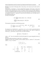
figure and self stress in a framework. We will now analyze a self-stressed
MLG (Fig. 7) in order to demonstrate the connection between self-stress
and singularity. Based on the definition of self stress framework, when a
bar-joint framework is in self stress, the sum of the forces of the bars
connected to a joint is equal to zero. Three equations corresponding to the
sum of forces in the three vertices 1,2,3 can be written as:
Sum of forces in vertex 1:
a+d+f =0
, (2)
Sum of forces in vertex 2:
b-d+e=0, (3)
Sum of forces in vertex 3:
c-e-f =0. (4)
These three equations are vector summations. We arbitrarily assign the
direction of the forces and consistently add the forces. Therefore, some of
the forces in Eq. 2-4 are negated. Summing Eq. 2, 3, and 4:
a+b+c=0
(5)
a
b
c
d
f
e
2
1

3
Figure 7. “Singular” (self stress) configuration of MLG
Equation 5 confirms a linear dependency of the three forces
a
,
b, and
c
.
These three forces are the forces corresponding to the lines of action of
the three limbs. The meaning of this dependency is that these three
limbs cannot generate instantaneous work (virtual work (Hunt, 1978)) on
the end-effector while it is moving in an instantaneous twist deformation
resulting from an external wrench applied on it. Therefore, self stress in
a framework is equivalent to a type-II singularity of a PPM. It is now
evident that the existence of a reciprocal figure indicates a self stress
framework, and in a similar way indicates a singular configuration in a
mechanism.
3.4 Locating the Singular Configurations
To find the configurations where there exists a reciprocal figure to a
particular PPM, and therefore it is in a singular configuration, one
should move the manipulator by changing its joint parameters while
tracking for configurations in which the reciprocal figure is visually
.
237
Graphical Singularity Analysis of 3-DOF PPMs
connected, e.g. in Fig. 6e, vertices p and q merge with p’ and q’
respectively. Figure 8 shows examples of PPM configurations in which
the reciprocal figure is connected and the manipulator is in a singular
configuration.
Figure 8. Two examples of singular configurations and the connected reciprocal

figures (3-R
PR left, 3-RRR right)
So far the search for a singular configuration was carried out by
changing the joint parameters of the manipulator and checking for the
existence of a connected reciprocal figure. If the analysis is constructed
the other way around, so that a connected reciprocal figure is first
constructed and only then an MLG is constructed to be reciprocal to it,
we can trace the loci of the singular configurations of the manipulator by
changing the reciprocal figure while keeping it connected (Fig. 9 left).
Note that the construction of the reciprocal figure in this case is based on
mechanical constraints of the PPM, e.g. the fixed shape of the end-
effector. Moreover, the singular configuration’s loci are traced relative to
a constant orientation of the PPM in order to enable us to plot the loci as
a 2-D graph. We refer the readers to (Sefrioui and Gosselin, 1995) to
examine the consistency of the results.
More examples, including JAVA applets of this method, can be found
at:
www.cs.cmu.edu/~adegani/graphical/
.
Figure 9. (Left) Singularity loci of 3-RPR in two different constant orientations
of the end-effector. (Right) A loci plot from six different orientations of the end-
effector (0,5, 10, 15, 20, and 25 degrees)
.
.
238 A. Degani and A. Wolf
4. Conclusion and Future Work
References
Bonev, I.A. (2002), Geometric analysis of parallel mechanisms. Ph.D. Thesis,
Laval University, Quebec, QC, Canada.
Crapo, H., and Whiteley, W. (1993), Plane self stresses and projected polyhedra I:

Gosselin, C., and Angeles, J. (1990), Singularity analysis of closed-loop kinematic
chains. IEEE Transactions on Robotics and Automation no. 3, vol. 6, pp. 281-
290.
C. Galletti, Advances in Robot Kinematics, Kluwer Acad. Publ., pp. 89-96.
Maxwell, J.C. (1864), On reciprocal figures and diagrams of forces. Phil. Mag no.
27, vol. 4, pp. 250-261.
Sefrioui, J., and Gosselin, C.M. (1995), On the quadratic nature of the
singularity curves of planar three-degree-of-freedom parallel manipulators.
Mechanism and Machine Theory no. 4, vol. 30, pp. 533-551.
Tsai, L.W. (1998), The Jacobian analysis of a parallel manipulator using
reciprocal screws, Proceedings of the 6th International Symposium on Recent
Advances in Robot Kinematics, Salzburg, Austria.
The graphical method which is presented and implemented in this paper
results in comparable outcomes to those obtained by other approaches
(e.g. Sefrioui and Gosselin, 1995), yet avoids some of the complexities in-
volved in analytic derivations. It is worth mentioning that the method we
present can be potentially applied to non-identical limb manipulators and
to other types of mechanisms as well. The method makes use of reciprocal
screws to represent the lines of action of PPMs’ limbs in a Mechanism’s
Line of action Graph (MLG), an insightful graphical representation of the
mechanism. Maxwell s theory of reciprocal figure and self stress is then
’
applied to create a dual figure of the MLG. Analyzing this dual (reciprocal)
the loci o
figure provides us with the singular configurations of the PPM and with
We are currently facing the challenge of expanding this graphical
able to use our relatively simple method to find the singular configura-
tions of complex three-dimensional manipulators, such as a 6-DOF
Gough-Stewart platform. One possible way to achieve this goal is to
method to the analysis of three-dimensional manipulators. We hope to be

project the spatial lines of action of the limbs on one or more planes
(Karger, 2004). We believe a self-stress analysis of these projected graphs,
similar to the one done on PPM, will offer insight into the singular confi-
guration of these non-planar manipulators.
The basic pattern. Structural Topology no. 1, vol. 20, pp. 55-78.
Hunt, K.H. (1978), Kinematic Geometry of Mechanisms, Oxford, Clarendon Press.
singular configurations of the manipulator. f
J. Lenarcic and
Karger, A. (2004), Projective properties of parallel manipulators,
^^
DIRECT SINGULARITY CLOSENESS
INDEXES FOR THE HEXA PARALLEL
ROBOT
Carlos Bier*, Alexandre Campos, J¨urgen Hesselbach
Institute of Machine Tools and Production Technology - TU Braunschweig
Langer Kamp 19b, 38106 Braunschweig, Germany
*
Abstract Direct kinematic singularities constrain the internal robot workspace
and the proximity to them must be detected online as fast as possible
for non deterministic trajectories. Direct singularity proximity for the
Hexa parallel robot is measured by means of three measure indexes with
two different physical bases. In this paper a new index based on Grass-
mann geometry to measure the singularity closeness is introduced. This
method and methods based on constraint minimization are applied and
validated in the Hexa robot. From the results we observe, for instance,
that the new index requires less time than the constraint minimization
methods but requires a better knowledge of the robot structure.
Keywords: Parallel Manipulator Singularities, Grassmann Geometry, Constrained
Minimization
1. Introduction

A measure of the direct singularity closeness for parallel manipulators
is required aiming at a safe operation space. For parallel robots as the
Hexa robot (Fig. 3d), workspace is limited by direct kinematic singu-
larities as well as by inverse kinematic singularities. Direct kinematic
singularities allow the end effector to gain unconstrained movements.
Its identification has been studied from different perspectives. The van-
ishing of the Jacobian determinant has been used for particular parallel
robots. However it is a product of factors and thus it suffers from the fact
that close to a singularity, where a factor shrinks to zero, other factors
may be big enough and the determinant does not indicate the singularity
closeness. Additionally, the physical meaning of the determinant is not
clear.
Qualitative conditions, based on Grassmann geometry, are proposed
to detect singularities of triangular simplified symmetric manipulators
[Merlet, 2000]. Quantitative approaches use a numerical measure to
determine how close a robot position is to a singularity. Different mea-
© 2006 Springer. Printed in the Netherlands.
J. Lenarþiþ and B. Roth (eds.), Advances in Robot Kinematics, 239–246.
239
-
sureshavebeenusedforthistask,e.g. the natural frequency measure
[Voglewede and Ebert-Uphoff, 2004], the power and the stiffness inspired
measure [Pottmann et al., 1998] based on a constraint minimization
In this paper a new method for quantitative measures of the direct
singularity closeness based on Grassmann geometry is presented. This
new method as well as the minimization based methods are applied to
the Hexa robot and the results are analyzed.
The six DOF Hexa robot is composed by six limbs connecting the
basis to the end effector, see Fig. 3d. Each limb contains an active
rotative joint A

i
(for i =1, ··· , 6). Its axes are fixed to the basis plane,
a passive universal joint B
i
and a passive spherical joint C
i
connected to
the end effector, so that all C
i
joints define the end effector plane. The
cranks and the passive links are connected at B
i
. The six limbs of the
Hexa robot are arranged in three pairs of two active joints with collinear
rotational axes. The pairs of active joints are axisymmetrical, i.e. 120
o
betweeneachpair.
2.
In spatial parallel manipulators the relationship between actuator co-
ordinates q and end effector Cartesian coordinates x can be stated as a
function f(q, x) = 0, where 0 is the 6-dimensional null vector. Therefore
the differential kinematic relation may be determined as
J
q
˙q − J
x
$
t
=0;J
q

˙q = J
x
$
t
(1)
where $
t
is the end effector velocity twist in ray order and, J
x
, J
q
and
J = J
−1
q
J
x
are the direct, inverse and standard Jacobian matrices, re-
spectively.
The rows of the direct kinematic matrix J
x
may correspond to the
normalized screw of wrenches, in axis order acting upon the end effec-
tor through the passive link, i.e. thedistallinkofeachlimb[David-
son and Hunt, 2004]. Therefore, a static relation may be stated as
J
T
x
τ =


ˆ
$
r1
, ··· ,
ˆ
$
r6

τ =$
r
,where$
r
is the result wrench acting upon
the end effector in axis order, τ =[τ
1
, ··· ,τ
6
] are the input wrench mag-
nitudes and the columns of J
T
x
are the normalized screws (axial order)
of wrenches acting on the end effector.
Singular configurations appear if either J
x
or J
q
drops rank. If J
x
is

singular, a direct singularity is encountered and the end effector gains
one or more uncontrollable degrees of freedom (DOF), on other hand if
240
matrix algebra.
method as well as the condition number [Xu et al., 1994] based on
Parallel anipulator Singularities
M
C. Bier, A. Campos and J. Hesselbach
J
q
drops rank it looses at least one DOF. The direct singularity occurs
in the workspace and is the main aim of this paper.
The new method as well as the minimization based methods are in-
troduced and applied to the Hexa robot.
3.
The constraint minimization method determines closeness to singu-
larity through an optimization problem that results in a corresponding
generalized eigenvalue problem. Using this methodology it is possible
to describe the instantaneous behavior of the end effector near singular-
ities for parallel manipulators in general [Voglewede and Ebert-Uphoff,
2004, Hesselbach et al., 2005]. In this approach, an objective function
F ($
t
) to be optimized is subject to move on a constraint h.Thisis
formulated mathematically as:
M(X)=

min/max F ($
t
)=$

T
t
J
T
SJ$
t
subject to h =$
T
t
T $
t
− c =0
(2)
where S (positive semidefinite) and T (positive definite) are n ×n sym-
metric matrix and c is some positive constant, e.g. c =1. Thesolution
of Eq. (2) gives the closeness measure to a singularity M(X)atapar-
ticular position and orientation X of the manipulator. The proposed
constrained optimization problem is found with the application of a La-
grange multiplier λ. The local extrema of the Lagrangian ζ($,λ)=
F ($
t
) − λh($
t
) are determined by its derivation. For a nontrivial solu-
tion to exist, the minimization (or maximization) of Lagrangian yields
det(J
T
SJ − λT ) = 0, which is called the corresponding general eigen-
value problem. The smallest eigenvalue λ
min

will be the minimum value
oftheobjectivefunctionF ($
t
), and so it can be utilized as a measure
value.
In general, this minimization problem was formulated based on an
arbitrary quantity for S and T [Voglewede and Ebert-Uphoff, 2004].
Taking J = J
x
, S = I
6x6
and T = diag[000111], then
√
λ
min
is associ-
ated to the minimum power [∼ W ] of the system, which indicates the
manipulator singularity closeness.
Another possible way is to choose S as the stiffness matrix of the
actuators K
Act
and T as the mass matrix of the manipulator M
EE
(or for
simplicity the end effector mass matrix, i.e. neglecting the limb masses).
Therefore,
√
λ
min
is associated to the ω natural frequency [∼ Hz]ofthe

system (M
EE
¨
X −ω
2
K
EE
= 0), indicating the singularity closeness.
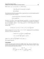
Both methods are applied in the Hexa robot (Fig. 3d) for its singu-
larity approximation measure. The measure behaviors of the minimum
power of the system through a singularity (Fig. 1a) is showed in Fig. 1b,
Direct Singularity Closeness Indexes for the Hexa Parallel Robot 241
Constraint inimization
M
here the end effector twists θ
o
around the $
min
(the end effector twist
which requires minimum power in this singularity). The singularity oc-
curs when
√
λ
min
= 0, but a singular range exists due to clearance and
compliance of the system, where the end effector is still unconstrained.
The singular range bound is experimentally identified as 0.029 ∼ W and
upon it the manipulator stiffness is warranted into the whole workspace.
q
$

tmin
20
30
40
50
60
70
80
0
20
40
60
80
q
angle
[°]
singular range
distance
[mm]
Grassmann algorithm V5b
limit value (55 mm)
singularity
V5b
c) d)
B
i
A
i
C
i

3
4
1
2
5
6
V5b
L
angle
[°]
q
0
10 20 30 40 50 60
0.01
0.02
0.03
0.04
singular range
power method
limit value (0.029 W)
~
singularity
V5a
power
(
)[
W
]
~
l

min
$
tmin
q
$
r1
$
r2
$
r3
$
r5
$
r4
a) b)
4
5
1
2
6
3
V5a
Figure 1. a) Grassmann variety V5a on the Hexa; b) Power based index; c) Grass-
man variety V5b; d) Grassman V5b based index
The same behavior is obtained through the frequency method. It is
important to notice that both methods detect all the singularities with
a unique index.
4. Grassmann Geometry
A new index to determine closeness to singularities is obtained based
on Grassmann geometry.

eties of lines, i.e. the sets of linear dependent lines to n given indepen-
dent lines, and characterized them geometrically according to their rank
(1, ··· , 6) [Hesselbach et al., 2005]. A singular configuration of the ma-
nipulator may be associated with a linear dependent set of lines, also
242
Grassmann (1809–1877) studied the vari-
C. Bier, A. Campos and J. Hesselbach
.
called line based singularities. In general, the reciprocal wrenches $
r
(Fig. 1a) to the passive twists of each manipulator leg are associated
to lines in the direction of the forces acting upon the end effector, also
called Pl¨ucker vectors. Linear dependence among these lines represents
a direct singularity. These wrenches compose the J
x
matrix (Sec. 2).
Using the Grassmann geometry we recognize that the Hexa robot may
be associated to several varieties. Some singularities of the Hexa robot
as well as correspondent varieties are shown in Figs. 1a, 1c and 2. In
the Hexa configurations of Fig. 2a, two wrenches are collinear and so $
r1
and $
r2
represent a Grassmann variety 1 (for short V1). Figure 2b shows
that four wrenches ($
r1
,$
r2
,$
r3

and $
r6
) are on a flat pencil V2b. Given
that the Hexa robot has six wrenches acting upon the end effector, the
configuration in Fig. 2a may be associated to V5a and the configuration
in Fig. 2b to V4d. In Fig. 2c all wrenches are parallel to each other and
they form a bundle of lines V3b. In Fig. 2d all wrenches lie in a plane
with different intersection points and represent a V3d. In Fig. 1a all
wrenches belong to a linear complex V5a, and Fig. 1c shows an example
where all wrenches are meeting one given line V5b. Each unconstrained
DOF of the end effector is represented by one $
min
in the Figs. 1a, 1c
and 2.
V2b
1
2
3
c) d)
$
tmin
$
tmin
$
tmin
$
tmin
$
tmin
$

tmin
$
r1
$
r2
$
r1
$
r2
$
r3
$
r6
$
r4
$
r5
a) b)
$
tmin
$
tmin
$
tmin
a
b
2
V1
1
V3b

1
2
3
4
1
2
3
4
V3d
Figure 2. Grassmann variety on the Hexa robot: a) V1; b) V2b; c) V3b; d) V3d
Considering the workspace of the Hexa robot which is limited by the
actuated joint angles, the possible Grassmann varieties may be reduced
to two: V5a and V5b. Thus only singularities of Fig. 1a and 1c may
Direct Singularity Closeness Indexes for the Hexa Parallel Robot 243
.
occur. With the help of the Grassmann geometry all possible singular
configurations on the Hexa robot are known. Aiming at quantify the
closeness to the singularities of Fig. 1a and Fig. 1c, a measure algorithm
is presented in the sequence.
A complex is generated by five skew symmetric lines (e.g. wrench
axes). Let π be a plane tangent to the complex that contains a point
of the line
B
6
C
6
(correspondent to the sixth wrench). The distance
between a certain point of this line and π gives a closeness measure to
that singularity. It is possible to build a 4×4 skew symmetric matrix G so
that B

T
i
GC
i
=0whereB
i
and C
i
(Fig. 1c) are in projective coordinates.
This linear system has six unknowns and five equations. For simplicity
and without loss of validity one unknown is set to 1. A pencil of lines of
the complex that contains B
6
defines π. Mathematically, if a projective
point X
p
=[xyz1]
T
= B
6
is an element of π,thenB
T
6
GX
p
=0.
Considering the vector U =[u
1
, ··· ,u
4

]
T
= B
T
6
G, the affine component
of plane is u
1
x + u
2
y + u
3
z + u
4
= 0. The distance between C
6
and π
may be interpreted as a measure for the line
B
6
C
6
of the complex:
d(C
6
,π)=v
1
C
6,x
+ v

2
C
6,y
+ v
3
C
6,z
+ v
4
=0;v
i
=
ui

u
2
1
+ u
2
2
+ u
2
3
(3)
If all the lengths
B
i
C
i
are the same and no other variety occurs,

d(C
6
,π) is a distance measure of the manipulator to a singularity V5a.
Singularity of V5b occurs if all six wrench axes
B
i
C
i
intersect one line
L. This line crosses two wrenches in the points C.Thesepointsmust
belong to legs whose drive axes are collinear and L must be parallel
to these drive axes. The maximal distance between L and all the six
wrenches is a measure to a singularity V5b of the Hexa robot.
This algorithm is applied in order to measure the closeness of the Hexa
robot to a singularity V5b as shown in Fig. 1c. The resulting distance
measure to the singularity is presented in Fig. 1d, where it linearly falls
down to zero in the singularity. Similarly to the minimization method,
a singular range is observed under the limit of 55 mm.
5. Conclusion
The Grassmann approach as well as the power and frequency meth-
ods are experimentally validated in the Hexa robot and investigated for
online singularity detection. All three methods allow a safe monitoring
of such positions and present some properties are described next.
movement (manually drived) from a rigid position, through a singularity
V5b and twice singularity V5a, to a rigid position. Figure 3a compares
244
The experiment presented in Figs. 3a and 3b shows the end effector
C. Bier, A. Campos and J. Hesselbach
both Grassmann algorithms with the power method and shows that a
Grassmann algorithm V5a does not detect a singularity of V5b and vice

versa. A combined Grassmann index, the lower of the both algorithms,
may be used due to that both present the same limit range of 55mm,
which is a general property. Comparing the combined Grassmann index
with the power and the frequency method in Fig. 3b, it can be observed
that all three methods have an equivalent behavior. It is important to
notice that a scale factor is required due to the different physical base
of each method. Additionally, it allows the use of a unique singularity
limit value.
2
4
6
8
10
12
0
time [s]
a)
20
40
60
80
100
120
b)
2
4
6
8
10
12

0
20
40
60
80
100
120
time [s]
singularity index
1900 x power [ W]~
combined Grassmann [mm]
38000 x frequency [ Hz]
~
1900 x power [ W]
~
Grassmann V5a [mm]
Grassmann V5b [mm]
singularity index
0
2
4681012
20
40
60
80
100
120
time [s]
computation time [µs]
power

frequency (simplified )M
EE
frequency (full )M
EE
combined Grassmann
c) d)
singularity
V5b
singularity
V5a
Figure 3. a) and b) Comparison of the singularity closeness indexes; c) Computa-
tional time; d) Hexa robot of Collaborative Research Center 562
For the online application of an approach, the computing time is a
decisive factor. For the same trajectory of example Fig. 3a, a comput-
ing time comparison is presented in Fig. 3c. The combined Grassmann
algorithm is notably faster than the minimization methods. Addition-
ally, in the frequency approach has been observed that using only the end
effector instead of the whole manipulator mass matrix M
EE
,thecompu-
tation time decreases without any loss of measure accuracy. Therefore,
it seems plausible to only use a simplified model of M
EE
.
Direct Singularity Closeness Indexes for the Hexa Parallel Robot 245
.
Properties as computational time, number of measured indexes, phys-
ical index meaning, method complexity and implementation costs must
to be considered to choose a suitable approach for a particular applica-
tion. The frequency method is general and can be applied to any type of

parallel manipulator. The drawback of this approach is its complexity
and that non-kinematic quantities (mass and stiffness) are introduced to
the measure. On the other hand the power approach does not present
this drawback and is not so complex. However, it can not detect fi-
nite and infinite (pure translation) unconstrained screw movements of
the end effector with the same index. Both minimization approach in-
dexes have a physical meaning in particular conditions (e.g. only unitary
wrenches acting upon the end effector), and generally they are only asso-
ciated to this physical meaning. The Grassmann approach offers a fast
and simple method to detect the singularities closeness with a geomet-
rical meaning index. The main weakness is that more than one index
is required if the robot presents more than one singular variety. It can-
not taken for granted that the measure index can be always combined
aiming at automatic singularity avoidance strategies.
In this paper, three singularity closeness indexes based on different
physical meanings, are evaluated in the Hexa robot. Each index is able
to detect all the direct singularities into the robot workspace. The prop-
erties of the new Grassmann based index are compared to the odder two
approaches and conclusions are presented.
References
Hesselbach, J., Bier, C., Campos, A., and L¨owe, H. (2005). Direct kinematic sin-
gularity detection of a hexa parallel robot. Proceedings - ICRA, pp. 3249-3254.
Barcelona.
Merlet, J. (2000). Parallel Robots. Kluwer Academic Publisher.
Pottmann, H., Peternell, M., and Ravani, B. (1998). Approximation in line space–
applications in robot kinematics and surface reconstruction. In Andvances in Robot
Kinematics, pp. 403-412, Salzburg. Kluwer Acad. Publ.
Sciavicco, L. and Siciliano, B. (1996). Modeling and Control of Robot Manipulators.
McGraw-Hill.
Tsai, L. (1999). Robot Analysis: the Mechanics of Serial and Parallel Manipulators.

John Wiley & Sons, New York.
Voglewede, P. and Ebert-Uphoff, I. (2004). Measuring closeness to singularities for
parallel manipulators. In Proceedings - ICRA, New Orleans.
Xu, Y. X., Kohli, D., and Weng, T. C. (1994). Direct differential kinematics of hybrid-
chain manipulators including singularity and stability analyses. Journal of Mechan-
ical Design, vol. 116, no. 2, pp. 614-621.
C
. Bier, A. Campos an
d
J. Hesse
lb
ac
h
24
6
Davidson, J. and Hunt, K. (2004). Robots and Screw The ory. Oxford University Press.
STEWART-GOUGH PLATFORMS WITH
SIMPLE SINGULARITY SURFACE
Adolf Karger
Charles University Praha
Faculty of Mathematics and Physics
Adolf.Karger@mff.cuni.cz
Abstract The singularity surface of a parallel manipulator is a very complicated
algebraic surface of high degree in six-dimensional space of all possible
positions of the manipulator (in the six-dimensional group of all space
congruences). In this paper we show that for some classes of manipula-
tors we can visualize the singularity set for any fixed orientation of the
manipulator by a quadric in the space of translations. Some properties
and examples are given.
Keywords: Stewart-Gough platforms, parallel manipulators, Study representation,

1. Introduction
is very complicated, in general it is given by 24 structural parameters
18 spatial coordinates of 6 points in the base and 18 in the platform, 12
of which can be specialized by using twice the congruence group, which
yields 12 parameters. This means that the description of the motion
leads to complicated equations and in general it is not possible to study
it in closed form.
To describe the singular set is still more complicated the general
equation of the singular set has about 10
6
terms and so it gives almost
no information about its properties. To obtain some closed form infor-
mation about singular positions of a parallel manipulator we have to
simplify the problem.
One possibility is to choose a fixed orientation of the platform and for
this orientation describe all singular positions. This can be done, but it
is easy to see that in this case we in general obtain a cubic surface in
E
3
, as the singularity surface is cubic in translations. Cubic surfaces in
space are still relatively complicated objects to give a good idea about
their shape. Using the general equation of the singular set we can show
that in case of S.
and base the equation of the singular set becomes only quadratical and
© 2006 Springer. Printed in the Netherlands.
247
J. Lenarþiþ and B. Roth (eds.), Advances in Robot Kinematics, 247–254.
singular positions
−
−

-
The geometry of a parallel manipulator of the type of S G. platform
G. platforms with affinely corresponding platform
therefore in this case the singular set for fixed orientation is given by a
quadric, which is much simpler to represent.
If the platform and base are affinely correspondent and planar, we get
much more specialized situation the singular set factorizes into three
factors either points of the platform lie on a conic section or the orien-
tation belongs to an algebraic hypersurface in the space of orientations
and the manipulator is singular for all translations or there is a plane of
singular positions (depending on the orientation). This describes the sit-
uation relatively well in both cases. It seems that the described situation
is not the only possibility for which the singular set is quadratical, but
the general solution seems to be difficult for non-planar base or platform.
This means to describe all parallel manipulators for which the singular
set is quadratical in translations. In the planar case the problem is not
difficult to solve, we show one example.
2. Description of the motion of a
Stewart
-Gough platform
Let g be a matrix of a space displacement,
g =

10
t
i
a
ij

(1)

parametrized by Euler parameters a
ij
= a
ij
(x
α
) and Study parameters
t
i
= t
i
(x
α
,y
β
),i,j =1, 2, 3,α,β =0, , 3 in the usual way, see Botema,
Roth, 1990, Husty, 1991, Husty, Karger, 2000, Karger, 2002.
We shall define the Study representation of the displacement group D
6
of the Euclidean space. We consider the 7-dimensional projective space
P
7
of the vector space R
8
with coordinates x
0
, , x
3
,y
0

, , y
3
. Points of
P
7
are determined by non-trivial 8-tuples (x
0
,x
1
,x
2
,x
3
,y
0
,y
1
,y
2
,y
3
)of
real numbers, given up to a nonzero multiple. From P
7
we remove the
subspace given by equations x
0
=0,x
1
=0,x

2
=0,x
3
=0, let P

7
be
the remaining part. Let S be the set in P

7
which is determined by the
equation
U = x
0
y
0
+ x
1
y
1
+ x
2
y
2
+ x
3
y
3
=0.
S will be called the Study quadric. We have a 1-1 correspondence

between points of S and elements of the group D
6
of space displacements.
To simplify computations we can normalize coordinates in S by the
requirement
K ≡ x
2
0
+ x
2
1
+ x
2
2
+ x
2
3
=1.
Now we shall describe the geometry of the motion of Stewart-Gough
platform. From kinematical point of view we can say that the upper
part of the platform lies in the moving space, the lower part lies in the
fixed space and the motion of the Stewart-Gough platform is generated
A. Karger248
−
−
by telescopic legs which connect six points of the moving space with six
points of the fixed space by spherical joints.
Let us suppose that we have chosen a system {O
1
,e

1
,e
2
,e
3
}
({O
2
,

f
1
,

f
2
,

f
3
}) of Cartesian coordinates in the moving (fixed) spaces,
respectively.
Let M =(A, B, C) be a point in the fixed space (lower part of the
platform), m =(a, b, c) be a point in the moving space (upper part of the
platform).
Any point m of the moving space can be also expressed by coordinates
(˜a,
˜
b, ˜c) with respect to the fixed space, where
˜a = t

1
+ a
11
a + a
12
b + a
13
c,
˜
b = t
2
+ a
21
a + a
22
b + a
23
c,
˜c = t
3
+ a
31
a + a
32
b + a
33
c.
The condition for the point m to lie on sphere with center at M and
radius r is
(˜a − A)

2
+(
˜
b − B)
2
+(˜c − C)
2
− r
2
=0.
In this equation we substitute Study parameters and the result is an
equation of degree four in x
i
,y
i
. This equation simplifies considerably
if we add 4U
2
to it. Then the factor K factorizes out and we obtain a
quadratical equation
h = RK +4(y
2
0
+ y
2
1
+ y
2
2
+ y

2
3
) −2x
2
0
(Aa + Bb + Cc)+
2x
2
1
(−Aa + Bb + Cc)+2x
2
2
(Aa −Bb −Cc)+2x
2
3
(Aa + Bb −Cc)+
4[x
0
x
1
(Bc −Cb)+x
0
x
2
(Ca − Ac)+x
0
x
3
(Ab −Ba) − x
1

x
2
(Ab + Ba)−
x
1
x
3
(Ac + Ca) −x
2
x
3
(Bc + Cb)+
(x
0
y
1
− y
0
x
1
)(A − a)+(x
0
y
2
− y
0
x
2
)(B − b)+(x
0

y
3
− y
0
x
3
)(C −c)+
(x
1
y
2
−y
1
x
2
)(C+c)−(x
1
y
3
−y
1
x
3
)(B+b)+(x
2
y
3
−y
2
x

3
)(A+a)] = 0, (2)
where R = A
2
+ B
2
+ C
2
+ a
2
+ b
2
+ c
2
−r
2
, Husty, 1991, Husty, Karger,
2000.
Let us suppose that the Stewart-Gough platform is given by six ar-
bitrary points M
i
=(A
i
,B
i
,C
i
) in the lower part and six points m
i
=

(a
i
,b
i
,c
i
) in the upper part of the platform, r
i
be also given, i =1, , 6.
We substitute coordinates of M
i
,m
i
in (2) and we obtain 6 equations
h
1
=0, , h
6
=0. (3)
By this way the geometry and kinematics of the platform is fully de-
scribed, Husty, 1991.
We would like to show how we can describe the singular positions
using the Study representation, because the reasoning is natural and
Stewart-Gough Platforms with Simple Singularity Surface
249
very simple. Let us suppose that r
i
are given as functions of time, r
i
=

r
i
(t). This generates a motion in the moving space described by a curve
x
i
= x
i
(t),y
i
= y
i
(t),i=0, , 3inP
7
. We express the velocity operator
for this motion. We can suppose that at instant t = t
0
the motion
passes through identity (the frame in the moving space is identical with
the frame in the fixed one),
10 00 j 0 j 0
The matrix of the motion is a function of the time, g = g(t)andfor
its derivative at t = t
0
we obtain
g

(t
0
)=2
⎛

⎜
⎜
⎝
0000
v
1
0 −u
3
u
2
v
2
u
3
0 −u
1
v
3
−u
2
u
1
0
⎞
⎟
⎟
⎠
, (4)
where u
j

= x

j
(t
0
),v
j
= y

j
(t
0
),j =1, 2, 3andx

0
(t
0
)=y

0
(t
0
)=0asa
consequence of K =1,U =0. The vector (u
1
,u
2
,u
3
) yields the rotational

part of the velocity operator, (v
1
,v
2
,v
3
) yields its translational part.
The derivative of (2) at t = t
0
yields
r(t
0
)r

(t
0
)/2=
u
1
(Bc−Cb)+u
2
(Ca−Ac)
+u
3
(Ab−Ba)+v
1
(A−a)+v
2
(B−b)+v
3

(C−c).
(5)
Application of this procedure to (3) yields a linear mapping φ which
transforms velocities (u
1
,u
2
,u
3
,v
1
,v
2
,v
3
) of the motion of the upper
part of the platform (end effector) into the linear velocities (r

1
, , r

6
)of
telescopic motions of legs of the manipulator. In practical problems we
more often need the inverse φ
−1
of this mapping, to express velocities
of the motion from velocities of legs. As we have 6 linear equations
for 6 unknowns, it exists iff the matrix of coefficients of φ is regular.
Coefficients are

(Bc −Cb,Ca − Ac, Ab − Ba,A − a, B −b, C −c), (6)
which are the Pl¨ucker coordinates of the line connecting points m and M.
Positions where φ is not invertible are called singular positions of the
parallel manipulator, see Botema, Roth, 1990, Karger, 2001, Karger,
2002, Ma, Angeles, 1992, Merlet, 1992.
3.
The singular surface is a very complicated hypersurface in the 6-
dimensional space of all possible configurations of the parallel manip-
ulator. It is of degree 10 in Study parameters and it has about 2000
A. Karger250
x (t )=1,y (t )=0,x (t )=y (t )=0,j =1, 2, 3.
Singular Set for Special arallel anipulators
P
M
terms in general for a given manipulator (with fully given geometry).
To give at least a partial idea how it looks like we shall concentrate at
special cases. We shall preserve translations as free parameters and use
Euler parameters for the orientation. We observe that the singular set
is of degree 3 in translations. This means that for given orientation of
the platform we obtain an algebraic surface of degree 3 in E
3
. Algebraic
surfaces of degree three were intensively studied but they have a rather
complicated structure. This is not very suitable for visualization or de-
scription. Therefore we shall concentrate at the case where the platform
and the base are affinely equivalent. In this case we observe that there
is a basic difference between the planar and nonplanar cases.
Let af first the platform (and base) be non-planar. We choose the
system of Cartesian coordinates in such a way that m
1

=[0, 0, 0],m
2
=
[a
2
, 0, 0],m
3
=[a
3
,b
3
, 0], and similarly for the base. We can suppose that
a
2
b
3
c
4
=0. Now let us suppose that there is an affine correspondence ψ
between the platform and base such that ψ(m
i
)=M
i
,i=1, , 6.ψis
X = f
11
x + f
12
y + f
13

z + f
1
,
Y = f
21
x + f
22
y + f
23
z + f
2
,
Z = f
31
x + f
32
y + f
33
z + f
3
,
where x, y, z are coordinates in the moving (platform) space, X, Y, Z are
coordinates in the fixed (base) space. Substitution of m
1
and M
1
yields
f
1
= f

2
= f
3
=0. Substitution of m
2
and M
2
yields f
11
= A
2
/a
2
,f
21
=
f
31
=0. From m
3
and M
3
we obtain
f
12
=
A
3
a
2

− A
2
a
3
a
2
b
3
,f
22
= B
3
/b
3
,f
32
=0.
The fourth pair of points m
4
and M
4
yields
A
4
= f
11
a
4
, +f
12

b
4
+
f
13
c
4
,
B
4
= f
22
b
4
+ f
23
c
4
,C
4
= f
33
c
4
and therefore
f
33
= C
4
/c

4
,
f
23
=
B
4
b
3
− B
3
b
4
b
3
c
4
,f
13
=
b
3
(A
4
a
2
− A
2
a
4

)+b
4
(A
2
a
3
− A
3
a
2
)
a
2
b
3
c
4
.
This finishes the computation of the affine correspondence and its equa-
tions are
X =
A
2
a
2
x +
A
3
a
2

− A
2
a
3
a
2
b
3
y +
b
3
(A
4
a
2
− A
2
a
4
)+b
4
(A
2
a
3
− A
3
a
2
)

a
2
b
3
c
4
z
Y =
B
3
b
3
y +
B
4
b
3
− B
3
b
4
b
3
c
4
z,Z =
C
4
c
4

z, (7)
Stewart-Gough Platforms with Simple Singularity Surface
251
Points M
5
,M
6
are determined by the correspondence ψ, because a spa-
tial affine correspondence is determined by four pairs of corresponding
points (in general position, which is our case). Let us write
Q =Σ
i,j,k
s
ijk
t
i
1
t
j
2
t
k
3
where the sum is over i, j, k,wherei ≥ 0,j ≥,k ≥ 0,i + j + k ≤ 3.
We suppose at first that s
ijk
= s
ijk
(a
α,β

), which means that we do not
substitute Euler parameters into coefficients of the orthogonal matrix
of the orientation, to keep the expression into reasonable limits. The
expansion of the equation of the singular set has then 164016 terms. We
obtain coefficients of degree three in Q of the following length given in
square brackets,
[s
300
] = 264, [s
030
] = 708, [s
003
] = 1224, [s
210
] = 1200, [s
201
] = 1590,
[s
102
] = 708, [s
021
] = 2484, [s
021
] = 2418, [s
012
] = 2928, [s
111
] = 3930.
Substitution from equations of the affine correspondence shows that
all these coefficients are equal to zero. This shows that for given orien-

tation the singular set is only a quadric in E
3
.
Example 1. We cho ose p oints
m
1
=[0, 0, 0],m
2
=[1, 0, 0],m
3
=[2, 1, 0],
m
4
=[3, 1, 1],m
5
=[5, 3, 6],m
6
=[5, 3, 4]
M
1
=[0, 0, 0],M
2
=[2, 0, 0],M
3
=[3, 2, 0],
M
4
=[1, 2, 2],M
5
=[−17, 6, 12],M

6
=[−9, 6, 8]
and orientation given by
x
0
=1/5,x
1
=2/5,x
2
= − 2/5,x
3
=4/5.
A. Karger252
The singular set can be seen at Fig. 1.
Figure 1. The singular set for non-planar platform from Example 1
4.
In the planar case we substitute C
i
= c
i
= 0 and the equation of
the singular set becomes shorter, it has 14640 terms (without Euler
Planar Platform and ase
B
.
q
1
= 0 can be explicitly solved as a linear sytem, but the solution is
too large to be given here. Instead of this we present an example of a
planar platform and base which are not affinely equivalent but they have

a singular set quadratical in translations.
Example 2. We write only first two coordinates of points.
m
1
=[0, 0],m
2
=[1, 0],m
3
=[2, 3],m
4
=[5, 7]
m
5
=[5, 8],m
6
=[12, 10],M
1
=[0, 0],M
2
=[2, 0],
M
3
=[3, 4],M
4
=[6, 8],M
5
=[3, 36/5],M
6
=[−2160/71, −2416/71].
The orientation is as in the first example. The singular set is at Fig. 2.

In the planar case the existence of an affine correspondence between
platform and base is more restrictive. Points M
4
,M
5
,M
6
are given by
the correspondence, as affine correspondence in the plane is determined
by three pairs of points. The equation for the singular set factorizes into
three factors, det(φ)=Q
1
.Q
2
.Q
3
.
Q
1
= 0 iff points m
i
lie on a conic section ( is known for a long
time), Q
2
= 0 depends only on the orientation of the platform and it
Stewart-Gough Platforms with Simple Singularity Surface
253
parameters). The equation of the singular set is still of third degree in
translations, but the cubic part factorizes into three factors,
t

3
[2t
1
(x
0
x
2
+ x
1
x
3
)+2t
2
(x
0
x
1
− x
2
x
3
)+t
3
(−x
2
0
+ x
2
1
+ x

2
2
− x
2
3
)]q
1
,
where q
1
is linear in t
1
,t
2
,t
3
with rather complicated coefficients, it is
not possible do display it here. This means that in general the singular
surface in the planar case remains cubic, but it has three asymtotic
planes. Let us have a look if the second factor can be equal to zero for
all directions. This yields equations
x
0
x
2
+ x
1
x
3
=0,x

0
x
1
− x
2
x
3
=0,x
2
0
+ x
2
3
= x
2
1
+ x
2
2
We obtain x
0
= r cos α, x
3
= r sin α, x
1
= r cos β, x
2
= r sin β, which
yields cos(α + β)=sin(α + β)=0, which is impossible. The equation
.

Figure 2. Singular set for the planar case from Example 2.
References
Husty, M.L., Karger A.: Self-motions of Griffis-Duffy type parallel manipulators. Pro-
ceedings of the 2000 IEEE international Conference on Robotics & Automation,
San Francisco, CA, April 2000, pp. 7-12.
2001.
Karger A.: Singularities ans Self-Motions of a special type of platforms. In J.Lernarˇciˇc
and F. Thomas, Advances in Robot Kinematics, Kluwer Acad. Publ. 2002, ISBN
0-7923-6426-0, pp. 355-364.
Ma O., Angeles J.: Architecture Singularities of Parallel Manipulators. Int. Journal
of Robotics and Automation 7, 23-29, 1992.
ometry. Int. Journal of Robotics Research, 8, 45-56, 1992.
A. Karger254
Bottema, O., Roth, B.: Theoretical Kinematics, Dover Publishing, 1990.
Husty, M.L.: An algorithm for solving the direct kinematics of general Stewart-Gough
platforms. Mech. Mach. Theory 31, 365-380, 1991.
Karger A.: Singularities and self-motions of equiform platforms. MMT 36, 801-815,,
,
Merlet, J.P.: Singular Configurations of Parallel Manipulators and Grasssmann Ge-
platform is singular for all translations. Q
3
= 0 is linear in translations.
We have
Q
2
=(A
3
a
2
− A

2
a
3
)(x
2
0
x
2
2
− x
2
1
x
2
3
)+(b
3
A
2
− B
3
a
2
)x
1
x
2
(x
2
0

+ x
2
3
)+
(b
3
A
2
+ B
3
a
2
)x
0
x
3
(x
2
1
+ x
2
2
)
Q
3
=2t
1
a
2
[x

1
x
3
(b
3
+ B
3
)+x
0
x
2
(b
3
− B
3
)]+
2t
2
[x
0
x
1
b
3
(A
2
− a
2
)+x
2

x
3
b
3
(A
2
+ a
2
)+(A
3
a
2
− A
2
a
3
)(x
0
x
2
− x
1
x
3
)]+
t
3
[2(A
3
a

2
− A
2
a
3
)(x
0
x
3
+ x
1
x
2
)+(b
3
− B
3
)(a
2
− A
2
)x
2
0
−
(b
3
+ B
3
)(a

2
− A
2
)x
2
1
− (b
3
− B
3
)(a
2
+ A
2
)x
2
2
+(b
3
+ B
3
)(a
2
+ A
2
)x
2
3
].
a plane. A special case was studied in Karger, 2001.

The research of this contribution was supported by research project
5. Conclusions
In this paper we have found a large class of parallel robot-manipulators
with the property that their singular set is at most quadratical in trans-
lations. In the non-planar case we have shown that this is true for
affinely equivalent base and platform. For planar platform and base the
In the planar
case it is also possible to find all manipulators which are quadratical in
translations, for the non-planar case the problem remains open.
MSM0021620839 of the Ministery of Education of the Czech Republic.
We see that in this case the singular set for given orientation is always
situation is much simpler. For affine equivalent platform and base the sin-
gular set factorizes into three factors two are independent of transla-
tions and the third one is only linear in translations.
Acknowledgements
is independent of translations. This means that if Q
2
=0, then the
,
Abstract The article presents an object-oriented representation of Frenet frame motion
along spatial curves in multibody systems. In this setting, the spatial track is
regarded as a kinetostatic transmission element transmitting motion and forces
as in a generic joint. It is shown that for the Frenet frame parameterization it is
possible to avoid singularities at the points of inflection by a special exponential
blending technique. The combination of the simple Frenet frame formulas with
singularity treatment leads to robust and efficient code for dynamic multibody
simulation. All concepts have been tested within an industrial application of
roller coaster design.
Keywords:
Guided motions along spatial curves have many applications in engineering

such as, for example, in the simulation of railways and roller coaster tracks, in
CNC machining (
ˇ
S´ır and J¨uttler, 2005), for guiding robot end effectors or for
describing the motion of bodies measured with tracking systems (Kecskem´ethy
et al., 2003).
While in unconstrained motion the path geometries for translation and ori-
entation are generated independently by dynamical equations, in guided mo-
accurately — termed fram ings. The framing of curves has been intensively
studied in previous works (Bishop, 1975, Hanson and Ma, 1995). A simple
© 2006 Springer. Printed in the Netherlands.
255
J. Lenarþiþ and B. Roth (eds.), Advances in Robot Kinematics, 255–264.
Spatial motion, Frenet frame, singularity treatment, kinematics
tion, one has to produce smooth trajectories that ensure good dynamic
behavior, and also create smooth rotation interpolations that follow the track
and computationally efficient frame parameterization uses the Frenet frame
with the axes oriented in tangential, normal and binormal direction, respec-
tively. Frenet curves have been used extensively in motion interpolation, rang-
ing from physics, e.g., to describe the motion of macromolecules (Balakrish-
nan and Blumenfeld, 1997) and to mechanical engineering, where they have
been used in constrained multibody systems using Lagrange equations of first
kind (Pombo and Ambrosio, 2003, Hansen and Elliott, 2002). One still un-
solved problem is that Frenet frames display a singularity when reaching points
of inflection, which limits their broad application. The framing suggested by
Bishop helps to circumvent this problem by minimizing angular velocity, but
on the other hand it requires the solution of a system of differential equations in
order to generate the trajectory, which is computationally expensive. The cur-
rent paper describes an approach for avoiding singularities of the Frenet frame
parameterizations and by this to provide a robust description that is suitable for

encapsulated code, such as required in object-oriented modelling. The avoid-
ance of singularities is achieved by a de l’Hospital limit analysis, allowing for
a continuous Frenet frame distribution even in the presence of points of zero
curvature.
The rest of the paper is organized as follows. Section 2 describes the idea
of object-oriented representation of multibody dynamics. This idea is applied
to spline joints in section 3. In the fourth section, the Frenet frame param-
eterization and the singularity treatment approach are described. Finally, the
application of the developed implementations to industrial roller-coaster de-
sign is presented.
For an object-oriented design, one requires a responsibility-driven approach
(Wirfs-Brock and Wilkerson, 1989) that allows for invoking complex software
by “clicking” at the elements. In mechanics, the most abstract “responsibility”
of mechanical components can be regarded to be the transmission of motion
and forces. In this view, a mechanical component acts as a kinetostatic trans-
mission element mapping motion and forces from one set of state objects —
the ‘input’ — to another set of state objects — the ‘output’ (Kecskem´ethy and
Hiller, 1994). Input and output state objects can be spatial reference frames
and/or scalar variables, including associated velocities, accelerations and gen-
eralized forces. Let the dimension of the input vector
be , and that of the
output vector
be . Then, the overall transmission behavior has the form
depicted in Fig. 1.
256
A Kecskeméthy and M. Tändl
Position
Velocity
Acceleration
Force

A simple transmission element.
The operation of motiontransmission consists of the three sub-operations
position:
velocity:
acceleration:
(1)
where
represents the Jacobian of the transmission element.
Furthermore, a force-transmission mapping can be defined by assuming that
the transmission element neither generates nor consumes power, i.e., that it is
ideal. Then, equating virtual work at the input and output yields
T
T
and, after substituting and noting that this condition must hold for
all
IR , one obtains the force transmission function
force:
T
(2)
Thus, in general, force transmission takes place in opposite direction to veloc-
ity transmission with the transposed velocity Jacobian. This relationship holds
independently of the complexity of the transmission element.
By the use of kinetostatic transmission elements, users can access the generic
properties of mechanical objects without having to refer to their internal imple-
mentation details. As shown in Kecskem´ethy and Hiller, 1994, it is possible to
generate all closure conditions of closed loops as well as the equations of mo-
tion of minimal order using only the basic kinetostatic transmission functions.
This allows one to combine models of mechanical elements without respect to
their internal complexity, making open-architecture, object-oriented libraries
possible (Kecskem´ethy, 2003).

In order to represent a guided motion as a kinetostatic transmission element,
one needs to identify inputs and outputs and describe the corresponding trans-
mission functions for motion and forces. Let a general curve be given as a
vector function
with respect to a basis frame in dependency of the
257
A Robust Model for 3D Tracking
path coordinate (Fig. 2). The coordinate frame may be located at some
spatial pose with respect to the inertially fixed coordinate system
.Themo-
tion along the curve is described by a moving frame
, which represents the
output of the kinetostatic transmission element. The inputs are embodied by
the reference frame
as well as the path coordinate .
Model of a spline joint.
In the following, we assume in general vectors to be decomposed in the
target frame, i.e., in the present case, in coordinates of
. For other decompo-
sitions, we introduce the notation
,where denotes the frame of decompo-
sition,
denotes the frame with respect to which the motion is measured, and
denotes the target frame. For motions measured with respect to frame ,the
index
is omitted. Likely, for decompositions in the target frame ,
the index
is omitted. Hence denotes the object . Furthermore, let
denote the derivative of a quantity with respect to the path coordinate ,andlet
denote the rotation matrix transforming coordinates with respect to frame

to coordinates with respect to frame . Then, the transmission behavior
of the spline joint can be defined by the following equations.
For the orientation and position of the output frame
, one obtains
T
(3)
depends on the framing of the curve as described in the next section.
Translational (
) and angular ( ) velocities of frame are obtained as
T
T T
(4)
258
A Kecskeméthy and M. Tändl
where is the rigid-body Jacobian, and is the Jacobian mapping path ve-
locity
to the velocity quantities of the output frame, as specified below for
the particular parameterization. Moreover, we employ the notation
for the
skew-symmetric matrix generated by a vector
T
as :
(5)
For the translational and angular acceleration, one obtains
(6)
According to the force transmission behavior for ideal transmission elements,
forces (
) and moments ( ) at the output frame are mapped to the correspond-
ing forces at the input frame. These are the force and moment at the frame
as well as the generalized force along the path coordinate. Hereby, the

force-moment wrench is assumed to be given with respect to the origin, and
all vectors are assumed to be decomposed in coordinates of the frame of refer-
ence. As shown in Kecskem´ethy and Hiller, 1994, this transmission is realized
by the transposed Jacobian:
T
T
(7)
For the generation of spatial curves, one can employ existing spline algorithms
from the literature. In the present context, the B-Spline routine of fifth order
from the spline library DIERCKX (Dierckx, 1993) was used.
The axes of the Frenet frame at path coordinate are the tangent vector
, the normal vector with curvature and
the binormal vector
. With , and being
the coordinate representations of , and in frame , the rotation matrix
becomes
(8)
For the Jacobian matrix , one obtains
(9)
A Robust Model for 3D Tracking
259
Frenet spline joint
where is the direction of the angular velocity of frame for and
is the tangent vector, and are the second and
third derivatives of
with respect to , all decomposed in . The acceleration
of
relative to is
(10)
At points of inflection, the standard formula for determining the normal

vector
fails, as both the nominator and the denominator vanish. However,
by a limit analysis, this difficulty can be overcome. Let the curvature
be described in the vicinity of the singularity by a linear approximation
with a still-to-be-determined positive constant . By substituting
for and using de l’Hospital’s rule, the right- and left-hand side
limits of
become, for ,
260
A Kecskeméthy and M. Tändl