Advances in Robot Kinematics - Jadran Lenarcic and Bernard Roth (Eds) Part 13 pps
Bạn đang xem bản rút gọn của tài liệu. Xem và tải ngay bản đầy đủ của tài liệu tại đây (1.03 MB, 30 trang )
Design of Mechanisms
W.A. Khan, S. Caro, D. Pasini, J. Angeles
architecture
D.V. Lee, S.A. Velinsky
Robust three-dimensional non-contacting angular motion sensor
K. Brunnthaler, H P. Schr¨ocker, M. Husty
Synthesis of spherical four-bar mechanisms using spherical
kinematic
mapping
R. Vertechy, V. Parenti-Castelli
Synthesis of 2-DOF spherical fully parallel mechanisms
G.S. Soh, J.M. McCarthy
Constraint synthesis for planar n-R robots
T. Bruckmann, A. Pott, M. Hiller
Calculating force distributions for redundantly actuated
tendon-
Stewart platforms
P. Boning, S. Dubowsky
A study of minimal sensor topologies for space robots
M. Callegari, M C. Palpacelli
Kinematics and optimization of the translating 3-CCR/3-RCC
parallel
mechanisms
359
369
377
385
395
403
413
423
based
Complexity analysis for the conceptual design of robotic
COMPLEXITY ANALYSIS
FOR THE
CONCEPTUAL DESIGN
OF ROBOTIC
ARCHITECTURES
Waseem A. Khan, St´ephane Caro, Damiano Pasini, Jorge Angeles
Department of Mechanical Engineering, McGill University
817, Sherbrooke St. West, Montreal, QC, Canada, H3A 2K6
{wakhan, caro}@cim.mcgill.ca, ,
Abstract We propose a formulation capable of measuring the complexity of kine-
matic chains at the conceptual stage in robot d esign. As an example,
two realizations of the Sch¨onflies displacement subgroup are compared.
Keywords: Conceptual design, complexity, kinematic chains, displacement sub-
groups
1. Introduction
We propose here a formulation capable of measuring the complexity
of the kinematic chains of robotic architectures at the conceptual-design
stage. The motivation lies in providing an aid to the robot designer
when selecting the best design alternative among various candidates at
the early stages of the design process, when a parametric design is not
yet available.
In this paper, the complexity of three lower kinematic pairs (LKPs),
the revolute, the prismatic and the cylindrical pairs, is first obtained.
Then, a formulation to measure the complexity of kinematic bonds
(Herv´e, 1978; Herv´e, 1999) is introduced. Based on this formulation,
the complexity of five displacement subgroups—the helical pair is left
out in this paper—is established. Finally, as an application, two realiza-
tions of the Sch¨onflies displacement subgroup (Angeles, 2004; Company
et al., 2001) are compared.
2. Kinematic Pair, Kinematic Bond
and
Kinematic Chain
A kinematic bond is defined as a set of displacements stemming from
the product of displacement subgroups (Herv´e, 1978; Angeles, 2004),
the bond itself not necessarily being a subgroup. We denote a kinematic
bond by L(i, n), where i and n stand for the integer numbers associated
© 2006 Springer. Printed in the Netherlands.
359
J. Lenarþiþ and B. Roth (eds.), Advances in Robot Kinematics, 359–368.
with the two end links of the bond. There are six basic displacement
subgroups R(A), P(e), H(A,p), C(A), F(u, v)andS(O)(Herv´e, 1978;
Herv´e, 1999; Angeles, 2004), each associated with a lower kinematic pair
(LKP). In this notation, A stands for the axis of the kinematic pair in
question; e, u and v are unit vectors, O is a point denoting the center
of the spherical pair; and p is the pitch of the helical pair.
A kinematic bond is realized by a kinematic chain. A kinematic chain
is the result of the coupling of rigid bodies, called links, via kinematic
pairs. When the coupling takes place in such a way that the two links
share a common surface, a lower kinematic pair results; when the cou-
pling takes place along a common line or a common point, a higher
kinematic pair is obtained. Examples of higher kinematic pairs include
gears and cams.
There are six lower kinematic pairs, namely, revolute R, prismatic
P, helical H, cylindrical C, planar F, and spherical S. These pairs can
be regarded as the generators of the six displacement subgroups listed
above. Although the displacement subgroups can be realized by their
corresponding LKPs, it is possible to realize some of their displacement
subgroups by appropriate kinematic chains. A common example is that
of the C(A) which, besides the C pair, can be realized by a suitable
concatenation of a P and a R pair.
3. The Loss of Regularity of a Surface
In this section, we propose a measure of the complexity of a given
surface. We base this measure on the concept of loss of regularity LOR,
defined as
LOR ≡
||κ
rms
||
2
||κ
rms
||
2
(1)
where κ
rms
is the r.m.s. of the two principal curvatures at a point of
the surface, κ
rms
is the derivative of κ
rms
with respect to a dimension-
less parameter σ. The LOR is inspired from Taguchi’s loss function
(Taguchi, 1993), and measures the diversity of the curvature distribu-
tion of the given surface, the LOR of the surfaces associated with five
lower kinematic pairs, being found below.
LOR of the Surface of the R Pair. Typically, the surface asso-
ciated with the revolute pair is assumed to be a cylinder. However, in
order to realize the R(A) subgroup, the translation in the axial direction
of the cylindrical surface must be constrained. This calls for additional
surfaces, which must then be blended smoothly with the cylindrical sur-
face in order to avoid curvature discontinuities.
360
W.A. Khan et al.
The above discussion reveals that the surface associated with a rev-
olute pair has to be a surface of revolution but cannot be an extruded
surface; the cylindrical surface is both. We should thus look for a gen-
eratrix G other than a straight line, but with G
2
-continuity everywhere.
The latter would allow a shaft of appropriate diameter to be blended
smoothly on both ends. The simplest realization of G is a 2-4-6 polyno-
mial, namely, P (x)=−x
6
+3x
4
− 3x
2
+1.
Figure 1(a) is a 3D rendering of the surface S
R
obtained by revolving
the generatrix G about the x-axis, so as to blend with a cylinder of unit
radius.
(a)
10
15
20
25
30
35
0 0.5
1 1.5
2
r
LOR
(b)
Figure 1. (a) A 3D rendering of the surface of revolution S
R
and (b) its LOR vs.
shaft radius r
The two principal curvatures of S
R
are given by (Oprea, 2004)
κ
µ
=
−y
(1 + y
2
)
3/2
,κ
π
=
1
y(1 + y
2
)
1/2
(2)
where y = P + r and r is the radius of the cylindrical shaft. The r.m.s.
of the two principal curvatures, κ
µ
and κ
π
, can now be obtained, i.e.,
κ
rms
=
1
2
(κ
2
µ
+ κ
2
π
)(3)
Next, we need to choose a suitable length parameter s and a homog-
enizing length l. A natural choice for s is the distance traveled along G;
l can be taken as the total length of the generatrix, the dimensionless
parameter being σ ≡ s/l.
The LOR of S
R
can now be evaluated by eq. (1),
Fig. 1(b). Notice that LOR
R
is not monotonic in r.Further,LOR
R
reaches a minimum of 10.2999 at r =0.1132. We thus assign LOR
R
=
10.2999.
Conceptual Design of Robotic Architectures
361
.
and depicted in
LOR of the Surface of the P P air. The most common cross
section of a P pair is a dovetail, but we might as well use an ellipse,
a square or a rectangle. A family of smooth curves that continuously
leads from a circle to a rectangle is known as Lam´e curves (Gardner,
1965). In their simplest form, these curves are given by x
m
+ y
m
=1,
where m>0isaneveninteger. Whenm = 2, the corresponding curve
is a circle of unit radius, with its center at the origin of the x-y plane.
As m increases, the curve becomes flatter and flatter at its intersections
with the coordinate axes, becoming more like a square. For m →∞,
the curve is a square of sides equal to two units of length and centered
at the origin. A Fourier analysis based on the curvature of these curves
confirms the intuitively accepted notion that the spectral richness, or
diversity, of the curvature increases with m (Khan, Caro, Pasini and
Angeles, 2006).
The LOR of the surface of the prismatic pair obtained by extruding
a square or a rectangle is expected to have a very high value. A Lam´e
curve L with m = 4 is plausibly the best candidate for the cross section
of the prismatic pair. This curve is shown in Fig. 2(a). Figure 2(b) is a
3D rendering of the surface S
P
obtained by extruding L along the z-axis.
–1
–0.5
0.5
1
–1
–0.5 0.5
1
y
x
s
(a) (b)
Figure 2. (a) Cross section of the prismatic pair; (b) A 3D rendering of the extruded
surface
The two principal curvatures of S
P
are given by
κ
µ
=
x
y
− y
x
(x
2
+ y
2
)
3/2
,κ
π
=0 (4)
The r.m.s. of the two principal curvatures, κ
µ
and κ
π
thus reduces to
κ
rms
= κ
µ
. The length parameter s and the homogenizing length l are,
correspondingly, the distance traveled along S
P
, depicted in Fig. 2(a),
and the total length l of the Lam´e curve, whence σ ≡ s/l.
The loss of regularity LOR
P
of S
P
, the surface associated with the P
pair, is thus LOR
P
=19.6802.
362
.
W.A. Khan et al.
LOR of the Surfac e of the F Pair. The F pair is a generator of
the planar subgroup F and requires two parallel planes, separated by
an arbitrary distance. In order to avoid corners and edges, a suitable
‘blending option’ is the use of the quartic Lam´e curve. The concept
is shown in Fig. 3(a). Notice that the female element of the pair is an
extruded surface S
Ff
while the male element is a solid of revolution S
Fm
.
–0.5
0.5
0.5
x,
y
d
D>>d
G
Fm
G
Ff
ξ
η
(a)
44
46
48
50
52
54
0 2
4
6 8 10
LOR
d
(b)
Figure 3. (a) Cross section of the simplest realization of the planar pair; (b) LOR
vs. diameter d of the male element
The LOR of the planar pair, LOR
F
, is defined by both the male and
the female elements. Further, the contribution of a flat surface to the
LOR is zero, a plane being a sphere of infinite radius. We thus obtain
LOR
plane
= lim
κ→0
||κ
rms
||
2
||κ
rms
||
2
= lim
κ→0
0
||κ
rms
||
2
=0 (5)
The LOR of the female element LOR
Ff
is thus the same as that of the
prismatic pair, that of the male element LOR
Fm
being evaluated below,
namely,
κ
µ
=
ξ
η
− η
ξ
(ξ
2
+ η
2
)
3/2
,κ
π
=
1
ξ
1+ξ
2
(6)
where, from Fig. 3(a), η = y and ξ = x + d/2, and d/2 is the dis-
tance between the y and the η axes. The length parameter s and the
homogenizing length l are, correspondingly, the distance traveled along
the generatrix G
Fm
depicted in Fig. 3(a) and its total length l, whence
σ ≡ s/l.
Figure 3(b) is a graph between the LOR of S
Fm
, LOR
Fm
,andthe
diameter d.NoticethatLOR
Fm
grows monotonically with d.Further,
LOR
Fm
reaches a limit of approximately 56.0399, whence LOR
Fm
=
56.0399. Finally, the LOR
F
is defined as
LOR
F
≡ (LOF
Ff
+LOF
Fm
)/2=
37.8601.
Conceptual Design of Robotic Architectures
363
.
LOR of the Surface of the C and S Pairs. The r.m.s. of the
principal curvatures of the cylindrical and the spherical surfaces is con-
stant. Hence, the loss of regularity is zero for the two surfaces, i.e.,
LOR
C
= LOR
S
=0.
4. The Geo metric Complexity of LKPs
We introduce here the geometric complexity of the LKPs based on the
LOR introduced earlier: the geometric complexity K
G|x
of a pair x is
K
G|x
≡
LOR
x
LOR
max
(7)
where LOR
x
is the loss of regularity of the surface associated with the
pair x and LOR
max
≡ max{LOR
R
,LOR
C
,LOR
P
,LOR
F
,LOR
S
}.The
geometric complexity of the five LKPs of interest is, in the foregoing
order: 0.2721; 0; 0.5198; 1.0; and 0.
5. The Complexity of Kinematic Bonds
In this section we lay the foundations for the evaluation of the com-
plexity of any kinematic bond. We first restrict our study to kinematic
bonds that are realizable using LKPs; the study of bonds including
higher kinematic pairs is as yet to be reported. Next, we define the
complexity K ∈ [0, 1] of a kinematic chain as a convex combination
(Boyd, 2004) of its various complexities:
K = w
J
K
J
+ w
N
K
N
+ w
L
K
L
+ w
B
K
B
(8)
where K
J
∈ [0, 1] is the joint-type complexity, K
N
∈ [0, 1] the joint-
number complexity, K
L
∈ [0, 1] the loop-complexity, and K
B
∈ [0, 1] the
bond-realization complexity, with w
J
, w
N
, w
L
,andw
B
denoting their
corresponding weights, such that w
J
+ w
N
+ w
L
+ w
B
=1.
5.1
J
Joint-type complexity is that associated with the type of LKPs used in
a kinematic chain. We define a preliminary joint-type complexity K
J|x
as the geometric complexity K
G|x
of the x pair, the joint-type complexity
K
J
of a kinematic bond L being defined as
K
J|L
=
1
n
(n
R
K
J|R
+ n
P
K
J|P
+ n
C
K
J|C
+ n
F
K
J|F
+ n
S
K
J|S
)(9)
where n
R
, n
P
, n
C
, n
F
and n
S
are the number of revolute, prismatic,
cylindrical, planar and spherical joints, respectively, while n is the total
number of pairs.
364
Joint-Type Complexity K
W.A. Khan et al.
5.2
N
The joint-number complexity K
N
is defined as that associated with a
kinematic bond L by virtue of its number of kinematic pairs, with respect
to the minimum required to realize the same set of displacements. We
adopt the expression
K
N|L
=1− exp(−q
N
N); N = n − m (10)
where n is the number of joints used in the realization of the bond L, m
is the minimum number of LKPs required to produce a displacement of
bond L ,andq
N
is the resolution parameter, to be adjusted according to
the resolution required. Note that K
N|L
∈ [0, 1].
5.3 Loop-Complexity K
L
The loop-complexity K
L|L
of a kinematic bond is that associated with
the number of independent loops of the kinematic chain connecting the
two links, i and n,ofakinematicbondL, with respect to the mini-
mum required to produce the prescribed displacement set. The loop-
complexity can be evaluated by means of the formula:
K
L|L
=1− exp(−q
L
L); L = l − l
m
(11)
where l is the number of kinematic loops, l
m
the minimum number of
loops required to realize such a bond and q
L
the resolution paramter.
5.4
B
The bond-realization complexity is associated with the geometric con-
straints involved in the realization of a kinematic bond. The complexity
of geometric constraints may be evaluated by the number of floating-
point operations (flops) required to realize a geometric constraint.One
flop is customarily defined as the combination of one addition and one
multiplication. Lack of space prevents us from including the flop analysis
of the geometric constraints, which is reported in (Khan, Caro, Pasini
and Angeles, 2006). A summary of the results of this analysis is dis-
played in Table 1.
The bond-realization complexity based on the geometric constraints
of its realization can now be defined as
K
B|L
=1− exp(−q
B
f) (12)
where f is the number of floating-point operations corresponding to the
constraints, q
B
being the corresponding resolution parameter.
Conceptual Design of Robotic Architectures
365
Joint-Number Complexity K
Bond-Realization Complexit y K
Table 1. Realization cost of some geometric constraints
Geometric constraint Representation flops total flops
Intersection of two lines (e
1
× e
2
) · q
21
=0 5A +9M 9
Angle of intersection e
1
· e
2
=cosα 2A +3M 3
Parallelism b/w tw o lines e
1
× e
2
= 0
3
3A +6M 6
Length of common normal ||q
21
− (q
21
· e
1
) e
1
||
2
2
= d
2
7A +9M 9
Intersection of three lines det(C)=0 30A +36M 36
e
1
, e
2
and e
3
span 3D space det([ e
1
e
2
e
3
]) =0 5A +9M 9
Definition of the resolution parameters. Three resolution para-
meters, namely q
N
, q
L
and q
B
were introduced above. These parameters
provide an appropriate resolution for the complexity at hand. Since the
foregoing formulation is intended to compare the complexities of two or
more kinematic chains, it is reasonable to assign a complexity of 0.9 to
the chain with maximum complexity and hence evaluate the normalizing
constant, i.e., for J = B, L, N,
q
J
=
− ln(0.1)/J
max
, for J
max
> 0;
0, for J
max
=0.
6. The Complexity of the Displacement
Subgroups
In Section 5, we assigned the joint-type complexity of the lower kine-
matic pairs as the geometric complexity of the surface associated with
the LKPs. The F pair requires the machining of two parallel planes,
separated by an arbitrary distance. Further, the F pair poses an ac-
cessibility problem to the male element of the coupling, this pair being
seldom used in practice as such. Moreover, precision spherical pairs are
expensive and difficult to manufacture.
Hence, using the geometric complexity of the LKPs as the correspond-
ing joint-type complexities is not justified. In order to solve this problem
we must look at the complexity of the displacement subgroups generated
by the five LKPs studied here.
The basic displacement subgroups can be realized either by their cor-
responding pairs or by a kinematic bond. The complexity of the dis-
placement subgroups is defined as the complexity of the realization that
exhibits the minimum kinematic bond complexity.
The complexity of the five displacement subgroups generated by the
LKPs considered here can now be evaluated. In this vein, we apply the
formulation introduced in the previous section to the different realiza-
tions of the displacement subgroups under study. Table 2 displays some
366
W.A. Khan et al.
.
Table 2. Complexity of five displacement subgroups
Subgroup Desc. K
J
K
N
K
B
K
R(A) R 0.2721/1 1 − e
−q
N
(0)
1 − e
−q
B
(0)
0.0907
P(e) P 0.5198/1 1 − e
−q
N
(0)
1 − e
−q
B
(0)
0.1733
C(A) C 0/1 1 − e
−q
N
(0)
1 − e
−q
B
(0)
0
PR 0.7919/2 1 − e
−q
N
(1)
1 − e
−q
B
(6)
0.4480
PPR 1.3117/3 1 − e
−q
N
(2)
1 − e
−q
B
(12)
0.5987
F(u, v) RRR 0.8163/3 1 − e
−q
N
(2)
1 − e
−q
B
(12)
0.5436
RPR 1.0640/3 1 − e
−q
N
(2)
1 − e
−q
B
(9)
0.5412
S( O) RRR 0.8163/3 1 − e
−q
N
(2)
1 − e
−q
B
(45)
0.6907
q
N
= − ln(0.1)/2=1.1513; q
B
= − ln(0.1)/45 = 0.0512
Table 3. Complexity of two realizations of the Sch¨onflies subgroup
Description K
J
K
N
K
L
K
B
K
McGill SMG 2.76/21 1 − e
−q
N
(21−2)
1 − e
−q
L
(5−0)
1 − e
−q
B
(258)
0.68
H4 16.79/22 1 − e
−q
N
(22−2)
1 − e
−q
L
(7−0)
1 − e
−q
B
(99)
0.79
q
N
= − ln(0 .1)/20 = 0.12; q
L
= − ln(0.1)/7=0.33; q
B
= − ln(0 .1)/258 = 0.01
pertinent realizations. The minimum complexity values found for R(A),
P(e), C(A), F(u, v)andS(O) are, correspondingly, 0.0907, 0.1733, 0,
0.5412 and 0.6907. Normalizing the above results so that the maxi-
mum is given a complexity of 1, we obtain the complexities of the five
displacement subgroups as
K
J|R
=0.1313,K
J|P
=0.2509,K
J|C
=0,K
J|F
=0.7836 (13)
Notice that, although these are not the joint-type complexity defined in
Section 5, which are rather based on form than on function,theabove
values can be used to evaluate the joint-type complexity in eq.(9).
7. Example
We apply our proposed formulation to compute the complexity of two
includes three independent translations and one rotation about an axis
of fixed orientation. Figure 4(b) shows the joint and loop graphs of the
McGill SMG (Angeles, 2005) and the H4 robot (Company et al., 2001).
Table 3 displays the different complexity values associated with the
topology of the two robots. Here, we note that the overall complexity
of the McGill SMG is lower than that of the H4 robot.
Conceptual Design of Robotic Architectures
367
motion capability of this subgroupSch¨onflies-motion generators. The
.
.
R
R
R
R
R
R
R
R
R
R
R
R
R
R
R
R
R
R
R
R
R
frame
tool
(a)
RR
R
R
RR
S
S
S
S
S
S
S
S
S
S
S
S
S
S
S
S
frame
tool
(b)
Figure 4. Joint and loop graphs of: (a) the McGill SMG; and (b) the H4 robot
8. Conclusions
The complexity analysis of kinematic chains at the conceptual stage
in robot design was proposed in this paper. To do this, the complexity
of five lower kinematic pairs and a formulation of the complexity of kine-
matic bonds were introduced. The complexity values of two realizations
of the Sch¨onflies displacement subgroup were computed.
References
Angeles, J. (2005). The degree of freedom of parallel robots: a grou p-theoretic ap-
proach. Proc. IEEE Int. Conf. Robotics and Automation, Barcelona, 1017–1024.
Angeles, J. (2004). The qualitative synthesis of parallel manipulators. ASME Journal
of Mechanical Design 126, 617–624.
Bo yd, S. and Vandenberghe, L. (2004). Convex Optimization. Cambridge University
Press, Cambridge.
Parallel Robot. European Patent EP1084802, March 21.
Gardner, M. (1965). T he superellipse: a curve that lies between the ellipse and the
rectangle. Scientific American, 213, 222–234.
Herv´e, J. (1978). Analyse structurelle des m´ecanismes par groupes de d´eplacements.
Mech. Mach. Theory 13, 437–450.
Herv´e, J. (1999). The Lie group of rigid body displacements, a fundamental tool for
mechanical design. Mech. Mach. Theory 34, 719–730.
Khan, W.A., Caro, S., Pasini, D. and Angeles, J. (2006). The Geometric Complexity
of Kinematic Chains. Department of Mechanical Engineering and Centre for In-
telligent Machine s Technical Report. CIM-TR 0601, McGill University, Montreal.
Oprea, J. (2004). Differential Geometry and its Applications. Pearson Prentice Hall,
New Jersey.
Taguchi, G. (1993). Taguchi on Robust Technology Development. Bringing Quality
Engineering Upstream. ASME Press, New York.
368
.
W.A. Khan et al.
Company, O., Pierrot, F., Shibukawa, T., and Koji, M. (2001). Four-Degree-of-Freedom
,
,
,
ROBUST THREE-DIMENSIONAL NON-
CONTACTING ANGULAR MOTION SENSOR
Danny V. Lee
Department of Mechanical and Aeronautical Engineering
University of California Davis
Steven A. Velinsky
Department of Mechanical and Aeronautical Engineering
University of California Davis
Abstract
Keywords:
1. Introduction
In the literature, there are a variety of devices based on a sphere
2003
, there is little work on spherical encoders or other means of three-
dimensional, orientation feedback without mechanical coupling.
In this paper, a non-contacting, angular velocity sensor based on
magnetometry is presented. The primary application for this sensor is a
ball wheel mechanism, which will serve as the drive train in a robust
omnidirectional mobile platform. Designed for operation in unstructured
environments, the spherical tire will be subject to contamination and
rotating in a cradle. These include: spherical motors as in Chirikjian and
For devices based on a sphere rotating in a cradle, the axis of rotation of the
sphere is arbitrary and can change instantaneously. Consequently, a non-
contact means of velocity sensing is desirable. For the ball wheel
mechanism, which serves as the drive train for a class of omnidirectional
mobile robots, most existing methods are not feasible, such as optical
techniques based on surface-pattern distinction. Thus, in this paper, a
robust, three-dimensional angular velocity sensor based on magnetometry is
presented that tracks the orientation of ferromagnet embedded in the
sphere. An algorithm based on vector orthogonality is used to approximate
the angular velocity vector of the sphere from the sampled orientation data.
Stein 1999, Dehez et al., 2005, spherical continuously variable trans-
missions as in Ostrowski 2000, Gillespie et al., 2002, and omni-
directional vehicles based on the ball wheel mechanism as in West and
Asada 1997, Ferriere et al., 2001. However, according to Stein et al.,
Motion-tracking, sensor, spherical motion
© 2006 Springer. Printed in the Netherlands.
369
J. Lenarþiþ and B. Roth (eds.), Advances in Robot Kinematics, 369–376.
wear. As a result, optical encoder techniques that require surface
tracking in demanding environments, magnetic sensing is commonly
invasive gastrointestinal transit monitoring.
Information on the configuration of a magnetic source provides a
means of determining the configuration of the body to which the sources
are attached. In this case, the goal is to determine the axis of rotation
and angular speed of the sphere given the absolute position of a point on
the sphere, which the magnetometry scheme provides. To solve this
1999
for applications in limb motion tracking in biomechanics.
2. Magnetometry Scheme
T
p
j
ˆ
k
ˆ
r
The proposed magnetometry scheme is based on tracking the magnetic
flux density vector of a cylindrically-symmetric ferromagnet, which will
be modeled as a magnetic dipole. Generally, the theoretical field
equations are a function of six configuration variables and physical
properties of the magnet. For this analysis it will be assumed that the
sphere and the magnet are both fixed in translation and both are
perfectly centered at the origin of an inertial reference frame.
370
D.V. Lee and S.A. Velinsky
contrast or surface patterning, as proposed by Garner et al., 2001, Stein
et al., 2003, are not feasible for this application. For non-contact motion
employed. Jacobs and Nelson 2001 use magnetic sensors to track
use magnetic sensing for vehicle guidance; and
Weitschies et al., 1994,
Figure 1. Schematic of field lines from magnetic dipole.
abdominal cavity deflection in crash test dummies; Donecker et al., 2003
loyed. This approach is described in
Panjabi 1979, Halvorsen et al., 1999
inverse problem, a method based on vector orthogonality will be emp-
Prakash and Spelman 1997 use magnetic marker tracking for non-
Consider the planar case as shown in Fig. 1. The magnet is located at
origin
m
O and the sensor is located at point . Unit vector defines the
magnet axis,
S
Op
ˆ
r is the position vector from
m
to
S
, andOO
T
is the relative
orientation between
r and . The magnetic flux density vectorp
ˆ
B is
decomposed into radial and tangential components and , and are,
respectively,
r
B
t
B
°
°
¿
°
°
¾
½
°
°
¯
°
°
®
T
S
P
T
S
P
sin
4
cos
2
3
0
3
0
r
M
B
r
M
B
t
r
, (1)
where
0
P
is the permeability and
M
is the dipole moment. The
relationship between the field components and the configuration
variables can be found in most texts on electromagnetic fields, such as
Shadowitz 1975. For the three-dimensional case, the expressions in Eq.
1 can be used in the plane defined by vectors and
p
ˆ
r . It remains, then, to
find the relationship between the radial and tangential field components
and the the three-dimensional, measured field components. A diagram of
the configuration is shown in Fig. 2.
p
ˆ
r
i
ˆ
j
ˆ
k
ˆ
T
r
e
ˆ
t
e
ˆ
n
e
ˆ
The magnetometer is positioned along the x-axis of the inertial reference
frame. This significantly simplifies the geometry of the problem.
{Bx,By,Bz} are the orthogonal field components from the magnetometer
Robust Three-Dimensional Non-Contacting Angular Motion Sensor
371
Figure 2. Sensor Diagram.
and {l,m,n} are the direction cosines used to parameterize the magnet
axis . Next, orthogonal triad is positioned at and defined as,
p
ˆ
}
ˆ
,
ˆ
,
ˆ
{
tnr
eee
S
O
°
¿
°
¾
½
°
¯
°
®
u
u
u
nrt
r
r
nr
eee
pe
pe
e
r
r
e
ˆˆˆ
,
ˆˆ
ˆˆ
ˆ
,
ˆ
. (2)
Unit vector
r
e is directed along the radial vector,
n
e is a unit vector normal
to the plane defined by and
ˆ
ˆ
p
ˆ
r , and
t
is the tangential unit vector in the
n
-plane, orthogonal to
r
. Moreover, the trigonometric functions in Eq.
1 can be expressed as a function of the direction cosines of ; as such,
e
ˆ
e
ˆ
e
ˆ
p
ˆ
°
¿
°
¾
½
°
¯
°
®
22
sin
cos
nm
l
T
T
. (3)
For an arbitrary orientation of , the theoretical magnetic flux density
vector can be expressed as,
p
ˆ
ttrr
TH
eBeBB
ˆˆ
. (4)
Eq. 2 and Eq. 3 provide the proper sign conventions through the
transformations. Substituting Eq. 1-3 into Eq. 4 results in the following
expression:
»
»
»
»
»
»
¼
º
«
«
«
«
«
«
¬
ª
#
»
»
»
¼
º
«
«
«
¬
ª
n
r
M
m
r
M
l
r
M
B
B
B
B
B
TH
M
z
y
x
M
3
0
3
0
3
0
2
4
2
S
P
S
P
S
P
. (5)
Eq. 5 states that the direction cosines of are linearly proportional to the
measured field components. In other words, this scheme directly
measures the motion of vector, fixed relative to the sphere, under
spherical motion. It remians to solve the inverse kinematics problem of
extracting the angular velocity vector of the sphere given this data.
p
ˆ
3. Inverse Kinematics of Spherical Motion
Calculating the angular displacement given the axis of rotation and
the trajectory of a point on the body, is a straightforward matter; several
orientation of the rotation axis and the angular displacement, given only
the trajectory of a point, is not well established. A method for estimating
displacements are used to locate the instantaneous axis of rotation for
D.V. Lee and S.A. Velinsky
372
techniques are shown in Murray et al., 1994. However, determining the
these values can be found in Halvorsen et al., 1999. In this work, two
represent a plane; the axis of rotation is defined by the intersection of
problem developed for post-processing. For applications in vehicle
tracking, a real-time method is necessary. The scheme presented below is
based on Halvorsen s concept of vector orthogonality but results from a
direct calculation of the on-line sampled data.
Perp
r
p
O
e
ˆ
Per p
'r
u
ˆ
'
u
ˆ
D
j
ˆ
i
ˆ
k
ˆ
p'
r
'r
e
ˆ
e
ˆ
r
ǚ
r
m
l
n
p
i
ˆ
j
ˆ
k
ˆ
O
(a) (b)
Fig. 3(a) is a diagram for the problem formulation. The position
S
ˆˆ
ˆ
Perp
r
e
Perp
Perp
Perp
Perp
ˆ
sin''
D
rrrr u . (6)
All the variables in Eq. 6 are unknown since the projections cannot be
Halvorsen’s work
Perp
r
can be replaced with a vectoru, which represents
the displacement of and calculated by normalizing its instantaneous
tangential velocity ; as such,
ˆ
p
p
r
r
v
v
u
p
p
ˆ
Robust Three-Dimensional Non-Contacting Angular Motion Sensor
373
limb motion. More specifically, each of these displacement vectors
Figure 3. Diagram for (a) general system kinematics and (b) planar sub-problem.
vector r of point p on sphere
is parameterized by the direction cosines
{l,m,n}, which is now a measured quantity from the magnetometry
scheme. As S rotates with angular velocity
ǚ , p follows the circular
arc C. Fig. 3(b) illustrates the vector relations of this motion; (r.e)e is
the projection of position vector
r along the axis of rotation, denoted
by unit vector
e , and projection is related to the other configu-
ration variables by:
made until the axis of rotation is determined. However, following
. (7)
,
,
these planes. Halvorsen s method involves a quadratic optimization
Substituting for u
ˆ
Perp
r
becomes,
eǂ'uu
ˆ
ˆˆ
u . (8)
Eq. 8 is often called the rotation vector for
D
is the radian rotation of u .
Dividing by the period T between samples results in the approximate
angular velocity vector; as such,
ˆ
ǚ(t)e
T
ǂ(t)
T
(t)uT)-(tu
|
u
ˆ
ˆˆ
. (9)
4. Experimental Verification
To verify this scheme a rod magnet rotated by a DC motor and an
Applied Physics Systems (APS) 535 fluxgate magnetometer was used to
track the resulting field. The magnet was positioned 6-inches from the
sensor origin. The rotation speed is stepped through a range of values for
comparison with the theoretical calculation. The maximum commanded
speed corresponds to a desired vehicle speed of approximately 5 mph.
The raw and filtered direction cosine data is shown in Fig. 4(a) and the
calculated tangential velocity components are shown in Fig. 4(b).
The raw data is processed with a second order Butterworth filter and the
differentiations were made using an ideal digital differentiator. While
these functions were chosen for convenience, the signal is always
sinusoidal in nature and therefore numerical differentiation of the on-
D.V. Lee and S.A. Velinsky
374
Figure 4. Experimental data for (a) position and (b) velocity.
and making a small angle approximation, Eq. 6
line sampled data is well-behaved. Fig. 5(a) is the radian rotation of the
magnet about the orthogonal axes of the inertial reference frame at each
sample, essentially the output of Eq. 8. The sensed speed compared to
the commanded speed is shown in Fig. 5(b).
10 20 30 40 50 60 70 80 90 100
0.04
0.035
0.03
0.025
0.02
0.015
0.01
0.005
0
0.005
Rotation [rad]
nx
ny
nz
(a) (b)
sensor were also carried out with equally promising results. A more
precise test fixture is being developed with optical encoders to track
transients as the axis of rotation changes orientation relative to the
sensor.
5. Conclusion
A three-dimensional, non-contacting, angular velocity sensor based on
magnetometry has been presented. The sensing scheme tracks the
orientation of the axis of a cylindrically-symmetric ferromagnet. A vector-
orthogonality approach is used to approximate the angular velocity
vector from the sampled orientation data. Initial feasibility testing has
clearly shown the potential of the approach.
References
Robust Three-Dimensional Non-Contacting Angular Motion Sensor
Figure 5. Sensor output (a) rotation vector and (b) angular speed.
y-axis of the magnetometer. Tests with the axis oriented relative to the
For the results presented, the axis of rotation was aligned with the
375
Chirikjian, G. S. and D. Stein (1999). Kinematic design and commutation of a
“
”
IEEE/ASME Transactions on Mechatronics 4(4): 342-353. spherical stepper motor.
–
–
–
–
–
–
–
–
Component of Rotation Vector
time [s]
A Mechatronic Sensing
32(11): 1221-1227.
“
”
“
”
Dehez, B., V. Froidmont, D. Grenier and B. Raucent (2005). Design, modeling
and first experimentation of a two-degree-of-freedom spherical actuator.
Donecker, S. M., T. A. Lasky and B. Ravani (2003).
System for Vehicle Guidance and Control. IEEE/ASME Transactions on Mecha-
tronics 8(4): 500-510.
Ferriere, L., G. Campion and B. Raucent (2001). ROLLMOBS, A New Drive
Garner, H., M. Klement and K. M. Lee (2001). Design and Analysis of an
Absolute Non-Contact Orientation Sensor for Wrist Motion Control. IEEE/
ASME International Conference on Advanced Intelligent Mechatronics, AIM 1: 69-74.
System for Omnimobile Robots. Robotica 19(1): 1-9.
“
”
“
”
Gillespie, R. B., C. A. Moore, M. Peshkin and J. E. Colgate (2002). Kinematic
Creep in a Continuously Variable Transmission: Traction Drive Mechanics for
Cobots. Transactions of the ASME Journal of Mechanical Design 124(4): 713-722.
”
Halvorsen, K., M. Lesser and A. Lundberg (1999). New Method for Estimating
the Axis of Rotation and the Center of Rotation. Journal of Biomechanics
Robotics and Computer-Integrated Manufacturing 21(3): 197-204.
“
“
”
Jacobs, B. C. and C. V. Nelson (2001). Development and Testing of a Magnetic Position
Sensor System for Automotive and Avionics Applications. Proceedings of SPIE -
The International Society for Optical Engineering.
Murray, R. M., Z. Li and S. S. Sastry (1994). A Mathematical Introduction to
Robotic Manipulation. Boca Raton, CRC Press.
Ostrowski, J. P. (2000). Controlling more with less using nonholonomic gears. 2000
IEEE/RSJ International Conference on Intelligent Robots and Systems,
Oct 31-Nov 5 2000, Takamatsu, Institute of Electrical and Electronics
Engineers Inc.
Panjabi, M. (1979). Center and angles of rotation of body joints: A study of errors
and optimization. Journal of Biomechanics 12(12): 911-920.
“
”
Prakash, N. M. and F. A. Spelman (1997). Localization of a Magnetic Marker for
GI Motility Studies: An In Vitro Feasibility Study. Proceedings of the 19th
Annual International Conference of the IEEE Engineering in Medicine and
Biology ociety.
Shadowitz, A. (1975). Electromagnetic Fields. New York, McGraw-Hill.
Stein, D., E. R. Scheinerman and G. S. Chirikjian (2003). Mathematical models
of binary spherical-motion encoders. IEEE/ASME Transactions on Mechatronics
8(2): 234-244.
“
”
Weitschies, W., J. Wedemeyer, R. Stehr and L. Trahms (1994). Magnetic
Transactions on Biomedical Engineering 41(2): 192-195.
Markers as a Noninvasive Tool to Monitor Gastrointestinal Transit. IEEE
“
”
West, M. and H. Asada (1997). Design of Ball Wheel Mechanisms for Omni-
directional Vehicles with Full Mobility and Invariant Kinematics. Transactions
of the ASME Journal of Mechanical Design 119(2): 153-161.
“
”
D.V. Lee and S.A. Velinsky
376
-
S
SYNTHESIS OF SPHERICAL FOUR-BAR
MECHANISMS USING SPHERICAL
KINE
Katrin Brunnthaler,
Hans-Peter Schr¨ocker,
Manfred Husty
University Innsbruck, Institute of Engineering Mathematics, Geometry and Computer
Science, Technikerstraße 13, A-6020 Innsbruck, Austria
, ,
Abstract Designing a spherical four-bar mechanism that guides a coupler system
through five given orientations is an old and well known problem. Here
we use kinematic mapping to solve the problem. We investigate the con-
straint surface belonging to a spherical RR-chain and solve the problem
in the newly defined kinematic design space. The algorithm results in
RR-chains which pairwise combined give the synthesized four-bars. It
is remarkable that with this method the univariate polynomial can be
computed completely general without specifying the parameters of the
problem with numerical values. Furthermore for the first time an exam-
ple with six real RR-chains is given. These can be combined to 30 real
four-bars that move the coupler system through the five given precision
points.
Keywords: Mechanism synthesis, spherical four-bar mechanism, five-orientations-
problem
1. Introduction
A spherical four-bar mechanism is a closed chain, which consists of
four bodies, linked by four revolute pairs incident with the same point.
One of the four bodies is called the base and is located in the fixed system
Σ
0
, which is connected with two links to the coupler, the moving system
Σ. Given five finitely separated orientations Σ
t
1
, ,Σ
t
5
of Σ (Fig. 1)
– sometimes called precision points – one can always find a finite set of
spherical RR-chains, guiding a coordinate system attached to the cou-
pler through them. To be more precise, one can find according to Roth,
1967 at most six real RR-chains, which are essentially different.
means, that solutions with axes origin-symmetric to axes of these RR-
chains are neglected. Six real RR-chains determine 30 different spherical
four-bar mechanisms, if there are just four, two or zero real RR-chains,
© 2006 Springer. Printed in the Netherlands.
MATIC MAPPING
That
377
J. Lenarþiþ and B. Roth (eds.), Advances in Robot Kinematics, 377–384.
Figure 1.
one can build only 12, one or zero spherical four-bar mechanisms guid-
ing a coordinate system attached to the coupler through the given five
orientations. Note, that not all orientations necessarily have to lie in
the same assembly branch of the spherical four-bar mechanism. There
exist a number of solutions of this synthesis problem, most of them use
kinematic properties of the motion itself. Bottema and Roth, 1979, Mc-
Carthy, 2000, Chiang, 1988, Lin, 1998, Dowler et al., 1978 solved the
problem via intersecting two center point curves to obtain the centers
respectively two circle point curves to obtain the circle points. These
points represent the points moving on circles in the synthesized spherical
four-bar motion. Bodduluri and McCarthy, 1992 solved this problem as
special case of a curve fitting method by minimizing a normal distance
in the image space. McCarthy, 2000 also solved this problem by using
a two-step elimination procedure that yields a sixth degree polynomial
in one of the coordinates of the fixed axes. In this paper the spherical
four-bar mechanism synthesis is solved in the kinematic image space of
spherical Euclidean displacements. We compute the constraint surface
representing a spherical RR-chain in this space and define then the kine-
matic design space which is sort of dual to the kinematic image space.
It turns out that in the kinematic design space the constraint surface
representing the design problem is a quadric surface with a very special
and simple structure. These geometric considerations are key to the
remarkable result that the univariate polynomial of degree six that gov-
erns this design problem can be derived completely general, i.e., without
specifying the coordinates of the five given orientations.
The paper is organized as follows: In Section 2 we give a brief intro-
duction to the mathematical framework and recall especially spherical
kinematic mapping. In Section 3 we derive the kinematic image of spher-
ical RR-chains and solve the synthesis problem using this representation.
378
K. Brunnthaler et al.
Given 5 orientations of a coordinate system
.
Section 4 illustrates the presented algorithm with a numerical example
that presents for the first time six real RR-chains.
2. Preliminaries
Spherical Euclidean displacements D can be described by
X = Ax, (1)
where X and x represent a point in the fixed and moving frame, re-
spectively and A ∈ SO(3) is a 3 × 3 proper orthogonal matrix (Husty
et al., 1997; McCarthy, 2000). For the following it is convenient to use
the Euler parameters to parameterize SO(3):
A :=
⎡
⎣
x
2
0
+ x
2
1
− x
2
3
− x
2
2
−2x
0
x
3
+2x
2
x
1
2x
3
x
1
+2x
0
x
2
2x
2
x
1
+2x
0
x
3
x
2
0
+ x
2
2
− x
2
1
− x
2
3
−2x
0
x
1
+2x
3
x
2
−2x
0
x
2
+2x
3
x
1
2x
3
x
2
+2x
0
x
1
x
2
0
+ x
2
3
− x
2
2
− x
2
1
⎤
⎦
.
(2)
In the matrix A the entries x
i
have been normalized so that x
2
0
+ x
2
1
+
x
2
2
+ x
2
3
=1. Themapping
κ : D→P ∈ P
3
A(x
i
) → (x
0
: x
1
: x
2
: x
3
) =(0:0:0:0) (3)
is called spherical kinematic mapping and maps each spherical Euclidean
displacement D to a point P in P
3
. The space P
3
is called kinematic
image space and is naturally endowed with an elliptic metric (Blaschke,
1960). It should be mentioned that x
i
are the components of the Hamil-
tonian quaternion which is associated with the corresponding element
of SO(3). Therefore one could also use the quaternion calculus as it is
done in McCarthy, 2000. The spherical kinematic mapping is the restric-
tion of the general spatial kinematic mapping to the orientation part of
the Euclidean displacement group. In spatial kinematic mapping each
Euclidean displacement D is mapped to a point P on a six dimensional
hyper-quadric S
2
6
⊂ P
7
. The spherical kinematic mapping restricts the
general one to a three dimensional subspace on S
2
6
.
3. Synthesis of Spherical Four-Bar Mechanisms
The spherical four-bar mechanism is a closed 4R-chain, where all four
revolute pairs intersect in one point. For the synthesis of such a mech-
anism we attach two of the revolute axes to the fixed system and two
axes to the moving (coupler) system. Now we prize open the coupler link
and obtain two open RR-chains. We map the possible displacements of
the first RR-chain into the spherical kinematic image space P
3
.This
379
Synthesis of Spherical Four-Bar Mechanisms
Figure 2.
yields the constraint manifold M
1
of the first RR-chain in the kinematic
image space. The same procedure we perform with the other RR-chain
and obtain a second constraint manifold M
2
. Possible assembly modes
of the two RR-chains correspond to intersection points of M
1
and M
2
.
These constraint manifolds will then be used for the synthesis algorithm.
3.1 Constraint Manifold of RR-Chains
In a spherical four-bar a point of the coupler revolute joint moves
on a circle. In Fig. 2 this is shown for the point M.ThepointM
is bound to this circle.
can say that point M is constrained to be on two spheres. One is the
unit sphere κ
0
the other is a sphere κ centered at piercing point M
0
of
the base the revolute joint with the unit sphere and radius r =
MM
0
.
Let the vector of the fixed revolute axis be v
f
=(A, B, C)
T
and the
corresponding vector of the moving revolute axis in the coupler system
be v
m
=(a, b, c)
T
. The endpoints of these vectors will be M
0
resp. M
when we have A
2
+ B
2
+ C
2
=1ora
2
+ b
2
+ c
2
=1. ThepathofM is
now modelled as the intersection curve of the two spheres:
κ
0
: X
2
1
+ X
2
2
+ X
2
3
− X
2
0
=0
κ : X
2
1
+ X
2
2
+ X
2
3
− 2AX
1
X
0
− 2BX
2
X
0
− 2CX
3
X
0
+ RX
2
0
=0. (4)
with R = A
2
+ B
2
+ C
2
− r
2
,wherer is the radius of the sphere and
A, B, C are the coordinates of the center. X
i
are the coordinates of
the moving pivot in the fixed system and can be computed via Eq. 1.
Substituting X =(X
0
,X
1
,X
2
,X
3
)
T
from Eq. 1 into Eq. 4 yields after
factorization:
(x
2
1
+ x
2
0
+ x
2
3
+ x
2
2
)(−2Ccx
2
3
− 2Aax
2
0
− 2Ccx
2
0
− 4Abx
0
x
3
+4Acx
0
x
2
+
4Bax
0
x
3
− 4Bcx
3
x
2
− 4Cax
0
x
2
− 4Cbx
3
x
2
+ a
2
x
2
0
+ a
2
x
2
3
+ a
2
x
2
2
K. Brunnthaler et al.
Four-bar and sphere
.
When we want to model this constraint we
380
b
2
x
2
2
+ c
2
x
2
3
+ b
2
x
2
0
+ b
2
x
2
3
+ c
2
x
2
0
+ c
2
x
2
2
+ x
2
1
c
2
+ x
2
1
a
2
+ x
2
1
b
2
+
Rx
2
0
+ Rx
2
3
+ Rx
2
2
+ x
2
1
R +2Bbx
2
3
+2Ccx
2
2
+2Aax
2
3
+2Aax
2
2
− 2Bbx
2
0
−
2Bbx
2
2
+2x
2
1
Cc − 2x
2
1
Aa +2x
2
1
Bb − 4x
1
Bcx
0
+4x
1
Cbx
0
− 4x
1
Abx
2
−
4x
1
Bax
2
− 4x
1
Acx
3
− 4x
1
Cax
3
)=0.
This equation can be simplified using the normalizing condition x
2
0
+
x
2
1
+ x
2
2
+ x
2
3
=1:
SCS :4Acx
0
x
2
− 4Abx
0
x
3
+4Bax
0
x
3
− 4Bcx
3
x
2
− 4Cax
0
x
2
− 4Cbx
3
x
2
−2Aa − 2Bb − 2Cc +4Bbx
2
3
+4Ccx
2
2
+4Aax
2
3
+4Aax
2
2
+4x
2
1
Cc
+
4x
2
1
Bb − 4x
1
Bcx
0
+4x
1
Cbx
0
− 4x
1
Abx
2
− 4x
1
Bax
2
− 4x
1
Acx
3
−4x
1
Cax
3
+ B
2
+ A
2
+ C
2
+ a
2
+ b
2
+ c
2
− r
2
=0. (5)
SCS is a quadratic surface (a hyperboloid) in P
3
and can be conve-
niently used for the analysis of spherical four-bar mechanisms following
the process demonstrated in Bottema and Roth, 1979 for planar four-bar
mechanisms. The four-bar motion is mapped to the intersection curve
of two hyperboloids in the image space and can easily be investigated
using the properties of the image space curve.
For the synthesis we have to adapt a different point of view. In the
synthesis some positions of a moving system are given and a mechanism
has to be synthesized. Therefore in Eq. 2 x
i
are known coefficients and
A, B, C, a, b, c, r are unknowns. Changing the point of view we have
now a seven dimensional design space DS having the coordinates A, B,
C, a, b, c, r and Eq. 2 is again a quadratic surface but now in the seven
dimensional design space. This surface is called design constraint surface
DCS and has the remarkable structure:
DCS : w
T
⎛
⎝
I −2B0
−2BI 0
0
T
0
T
−1
⎞
⎠
w =0 (6)
where the coordinates of DS are assembled to a vector w =(A, B, C, a, b,
c, r)
T
, I is the three dimensional unit matrix, B is the right lower 3 ×3-
matrix in matrix A (Eq. 1) and 0 is a 3-dimensional zero vector. From
this representation we see immediately that the squared coordinates of
DCS are free of the position parameters x
i
. This will be crucial in the
synthesis algorithm below.
3.2 Synthesis Algorithm
Given are five precision points P
1
, P
2
, P
3
, P
4
and P
5
∈ P
3
s
ponding to five orientations of a coordinate system. The goal is to
Synthesis of Spherical Four-Bar Mechanisms
, corre -
381
+
compute the design parameters A, B, C, a, b, c, r of the spherical mecha-
nism that guides the coupler system through these orientations. It is evi-
dent from the section before that the five precision point yield five design
constraint equations DCS
i
,i =1, ,5. Furthermore we have two nor-
malizing equations N
1
: A
2
+ B
2
+ C
2
−1=0,N
2
: a
2
+ b
2
+ c
2
−1=0.
DCS
i
and N
i
constitute a system of seven nonlinear equations to solve
the synthesis problem. N
i
are free of position parameters, therefore they
will be used at the very end of the the synthesis algorithm to normalize
the solution vectors.
Without loss of generality we can assume that the fixed system Σ
0
coincides with one of the five given orientations. Otherwise there exists
a unique Euclidean transformation, which does not change the design of
the mechanism, to obtain this situation. Thus, the image space point,
which represents the identity
(x
0
: x
1
: x
2
: x
3
)=(1:0:0:0) (7)
has to be on one design constraint manifold:
DCS
1
:= −2Bb−2Cc−2Aa +A
2
+ C
2
+ B
2
+ a
2
+ b
2
+ c
2
−r
2
=0. (8)
Now four simple equations are built by subtracting DCS
1
from the other
four constraint equations:
M
1j
= DCS
j
− DCS
1
,j=2, 5.
The four difference equations are bilinear in the unknowns A, B, C, a,
b, c and do not contain r. Note that at least one of the unknowns in
(A, B, C)and(a, b, c) has to be non zero. Let us assume that C and
c are nonzero. Therefore we can set for the moment C =1,c =1.
We emphasize that this is no restriction of generality. Now we have
four simple bilinear equations M
1j
. Two of these equations, say M
1,2
and M
1,3
are used to solve linearly for two of the unknowns, say a, b.
The solutions are substituted into M
1,4
and M
1,5
. Thisyieldstwocubic
equations C
1
,C
2
. The resultant of C
1
,C
2
with respect to one of the
remaining unknowns, say B yields a univariate polynomial Q
9
of degree
nine in the unknown A. Q
9
factors into the solution polynomial Q
6
of degree six and in three linear factors. The linear factors are not
solution of the system because they would cause the determinant of
the linear system to vanish. This proposition can be proven easily by
computing the resultant of the determinant polynomial of the linear
system (M
1,2
,M
1,3
)ande.g.C
1
. The linear factors are contained in
the ideal spanned by these two equations. Therefore they have to be
cancelled.
K. Brunnthaler et al.
382