Artificial Mind System – Kernel Memory Approach - Tetsuya Hoya Part 3 potx
Bạn đang xem bản rút gọn của tài liệu. Xem và tải ngay bản đầy đủ của tài liệu tại đây (478.53 KB, 20 trang )
208 10 Modelling Abstract Notions Relevant to the Mind
2
1
.
.
.
.
.
.
v
3
v
2
v
L
o
o
LTM,2
LTM,3
LTM,L
o
c
o
n
D
i
s
i
U
n
i
t
e
(HA−GRNN
Output)
o
NET
v
1
o
LTM,1
Input
STM
Direct Paths to
LTM Net 1
x
LTM
LTM
LTM
LTM
Net 1
Net 2
Net 3
Net L
o
STM
(Self−Evolution Process)
(intuitive output)
the RBFs in
Fig. 10.4. The hierarchically arranged generalised regression neural network (HA-
GRNN) – modelling the notion of attention, intuition, LTM, and STM within the
evolutionary process of the HA-GRNN. As the name HA-GRNN denotes, the model
consists of a multiple of dynamically reconfigurable neural networks arranged in a
hierarchical order, each of which can be realised by a PNN/GRNN (see Sect. 2.3)
or a collection of the RBFs and the associated mechanism to generate the output
(i.e. for both LTM Net 1 and the STM)
Then, in Fig. 10.4, x denotes the incoming input pattern vector to the
HA-GRNN, o
STM
is the STM output vector, o
LT M,i
(i =1, 2, ,L)arethe
LTM network outputs, v
i
are the respective weighting values for the LTM
network outputs, and o
NET
is the final output obtained from the HA-GRNN
(i.e. given as the pattern recognition result by 3) above).
The original concept of the HA-GRNN was motivated from various studies
relevant to the memory system in the brain (James, 1890; Hikosaka et al.,
1996; Shigematsu et al., 1996; Osaka, 1997; Taylor et al., 2000; Gazzaniga
et al., 2002).
10.6.2 Architectures of the STM/LTM Networks
As in Fig. 10.4, the LTM networks are subdivided into two types of networks;
one for generating “intuitive outputs” (“LTM Net 1”) and the rest (“LTM
Net 2 to LTM Net L”) for the regular outputs.
For the regular LTM, each LTM Net (2 to L) is the original PNN/GRNN
(and thus has the same structure as shown in the right part of Fig. 2.2, on
10.6 Embodiment of Attention, Intuition, LTM, and STM Modules 209
activated RBF
the most
Selection of
.
.
.
h
1
STM
o
h
2
h
M
x
Fig. 10.5. The architecture of the STM network – consisting of multiple RBFs and
the associated LIFO stack-like mechanism to yield the network output. Note that
the STM network output is given as a vector instead of a scalar value
(winner−take−all
strategy)
Decision Unit
.
.
.
h
1
h
2
h
M
x
LTM,1
o
Fig. 10.6. The architecture of LTM Net 1 – consisting of multiple RBFs and the
associated mechanism to yield the network output (i.e. by following the “winner-
takes-all” strategy)
page 15), whereas both the STM and LTM Net 1 consist of a set of RBFs and
the associated mechanism to generate the output from the network (alterna-
tively, they can also be seen as modified RBF-NNs) as illustrated in Figs. 10.5
and 10.6, respectively. As described later, the manner of generating outputs
from STM or LTM Net 1 is however different from ordinary PNNs/GRNNs.
Although both the architectures of the STM and LTM Net 1 are similar
to each other, the difference is left within the manner of yielding the network
output; unlike ordinary neural network principle, the network output of the
STM is given as the vector obtained by the associated LIFO stack-like mech-
anism (to be described later in Sect. 10.6.4), whilst that given by LTM Net 1
is a scalar value as in ordinary PNNs/GRNNs.
10.6.3 Evolution of the HA-GRNN
The HA-GRNN is constructed by following the evolutionary schedule which
can be subdivided further into the following five phases:
210 10 Modelling Abstract Notions Relevant to the Mind
[Evolutionary Schedule of HA-GRNN]
Phase 1: The STM and LTM Net 2 formation.
Phase 2: Formation/network growing of LTM Nets (2 to L).
Phase 3: Reconfiguration of LTM Nets (2 to L) (self-evolution).
Phase 4: Formation of LTM Net 1 (for generating intuitive outputs).
Phase 5: Formation of the attentive states.
Phase 1: Formation of the STM Network and LTM Net 2
In Phase 1, the STM network is firstly formed (how the STM network is
actually formed will be described in detail in Sect. 10.6.4), and then LTM Net
2 is constructed by directly assigning the output vectors of the STM network
to the centroid vectors of the RBFs in LTM Net 2. In other words, at the
initial stage of the evolutionary process (i.e. from the very first presentation
of the incoming input pattern vector until LTM Net 2 is filled), since each
LTM network except LTM Net 1 is represented by a PNN/GRNN, the RBFs
within LTM Net 2 are distributed into the respective sub-networks, according
to the class “label” (i.e. the label is set by the target vector consisting of a
series of indicator functions as defined in (2.4); cf. also Fig. 2.2, on page 15)
associated with each centroid vector.
Phase 2: Formation of LTM Nets (2 to L)
The addition of the RBFs in Sub-Net i (i =1, 2, ,N
cl
, where N
cl
is the
number of classes which is identical to the number of the sub-nets in each
LTM network
5
) of LTM Net 2 is repeated until the total number of RBFs in
Sub-Net i reaches a maximum M
LT M
2
,i
(i.e. the process can be viewed as the
network growing). Otherwise, the least activated RBF in Sub-Net i is moved
to LTM Net 3. Then, this process corresponds to Phase 2 and is summarised
as follows:
[Phase 2: Formation of LTM Nets (2 to L)]
Step 1)
Provided that the output vector from the STM network
falls into Class i,forj =1toL−1, perform the following:
If the number of the RBFs in Sub-Net i of LTM
Net j reaches a maximum M
LT M
j,i
,movethe
least activated RBF within Sub-Net i of LTM
Net j to that of LTM Net j +1.
5
Here, without loss of generality, it is assumed that the number of the sub-nets
isuniqueineachofLTMNets(2toL).
10.6 Embodiment of Attention, Intuition, LTM, and STM Modules 211
Step 2)
If the number of the RBFs in Sub-Net i of LTM
Net L reaches a maximum M
LT M
L,i
(i.e. all the i-th
sub-networks within LTM Nets (2 to L) are filled), there
is no entry to store the new output vector. Therefore,
perform the following:
Step 2.1) Discard the least activated RBF in Sub-Net
i of LTM Net L.
Step 2.2) Shift one by one all the least activated RBFs
in Sub-Net i ofLTMNets(L-1to2)intothatof
LTM Nets (L to 3).
Step 2.3) Then, store the new output vector from the
STM network in Sub-Net i of LTM Net 2.
(Thus, it can be seen that the procedure above is
also similar to a last-in-first-out (LIFO) stack; cf.
the similar strategy for the STM/working memory
module described in Sect. 8.3.7.)
The above process is performed based on the hypothesis that long-term
memory can be represented by a layered structure, where in the HA-GRNN
context the (regular) long-term memory is represented as a group of LTM Nets
(2 to L), and that each element of memory is represented by the corresponding
RBF and stored in a specific order arranged according to the contribution to
yield the final output of the HA-GRNN.
In Fig. 10.4, the final output from the HA-GRNN o
NET
is given as
the largest value amongst the weighted LTM network outputs o
LT M,i
(i =
1, 2, ···,L):
o
NET
= max(v
1
× o
LT M,1
,v
2
× o
LT M,2
, ,v
L
× o
LT M,L
), (10.3)
where
v
1
>> v
2
>v
3
> >v
L
. (10.4)
Note that the weight value v
1
for o
LT M,1
must be given relatively larger
than the others v
2
,v
3
, ,v
L
. This discrimination then urges the formation
of the intuitive output from the HA-GRNN to be described later.
Phase 3: Reconfiguration of LTM Nets (2 to L) (Self-Evolution)
After the formation of LTM Nets (2 to L), the reconfiguration process of
the LTM networks may be initiated in Phase 3, in order to restructure the
LTM part. This process may be invoked either at a particular (period of)
time or due to the strong excitation of some RBFs in the LTM networks by
212 10 Modelling Abstract Notions Relevant to the Mind
a particular input pattern vector(s)
6
. During the reconfiguration phase, the
presentation of the incoming input pattern vectors from the outside is not
allowed to process at all, but the centroid vectors obtained from the LTM
networks are used instead as the input vectors to the STM network (hence
the term “self-evolution”). Then, the reconfiguration procedure within the
HA-GRNN context is summarised as follows:
[Phase 3: Reconfiguration of LTM Nets (2 to L)
(Self-Evolution)]
Step 1)
Collect all the centroid vectors within LTM Nets 2 to l
(l ≤ L), then set them as the respective incoming pattern
vectors to the HA-GRNN.
Step 2)
Present them to the HA-GRNN, one by one. This process
is repeated p times. (In Fig. 10.4, this flow is depicted
(dotted line) from the regular LTM networks to the STM
network.)
It is then considered that the above reconfiguration process invoked at a
particular time period is effective for “shaping up” the pattern space spanned
by the RBFs within LTM Nets (2 to L).
In addition, alternative to the above, such a non-hierarchical clustering
method as in (Hoya and Chambers, 2001a) may be considered for the re-
configuration of the LTM networks. The approach in (Hoya and Chambers,
2001a) is, however, not considered to be suitable for the instance-based (or
rather hierarchical clustering) operation as above, since, with the approach
in (Hoya and Chambers, 2001a), a new set of the RBFs for LTM will be ob-
tained by compressing the existing LTM using a clustering technique, which,
as reported, may (sometimes) eventually collapse the pattern space, especially
when the number of representative vectors becomes small.
Phase 4: Formation of LTM Net 1
In Phase 4, a certain number of the RBFs in LTM Nets (2 to L) which keep
relatively strong activation in a certain period of the pattern presentation are
transferred to LTM Net 1. Each RBF newly added in LTM Net 1 then forms
a modified PNN/GRNN and will have a direct connection with the incoming
input vector, instead of the output vector from the STM. The formation of
LTM Net 1 is summarised as follows
7
:
6
In the simulation example given later, the latter case will not be considered due
to the analytical difficulty.
7
Here, although the LTM is divided into the regular LTM networks (i.e. LTM
Nets 2 to L) and LTM Net 1 for generating the intuitive outputs, such a division
10.6 Embodiment of Attention, Intuition, LTM, and STM Modules 213
[Phase 4: Formation of LTM Net 1]
Step 1)
In Phases 2 and 3 (i.e. during the formation/reconfiguration
of the LTM Nets (2 to L)), given an output vector from the
STM, the most activated RBFs in LTM Nets (2 to L) are
monitored; each RBF has an auxiliary variable which is ini-
tially set to 0 and is incremented, whenever the correspond-
ing RBF is most activated and the class ID of the given
incoming pattern vector matches the sub-network number
to which the RBF belongs.
Step 2)
Then, at a particular time or period (q, say), list up all the
auxiliary variables (or, activation counter) of the RBFs in
LTM Nets (2 to L) and obtain the N RBFs with the N
largest numbers, where the number N canbesetas
N<<
i
j
M
LT M
j,i
(j =2, 3, , L).
Step 3)
If the total number of RBFs in LTM Net 1 is currently
less than or equal to M
LT M
1
− N (i.e. M
LT M
1
denotes the
maximum number of the RBFs in LTM Net 1, assuming
N ≤ M
LT M
1
), move all the N RBFs to LTM Net 1. Oth-
erwise, retain the original M
LT M
1
− N RBFs within LTM
Net 1 and fill/replace the remaining RBFs in LTM Net 1
with the N newly obtained RBFs.
Step 4)
Create a direct path to the incoming input pattern vector
for each RBF added in the previous step
8
. (This data flow is
illustrated (bold line) in Fig. 10.4.) The output of LTM Net
1 is given as a maximum value within all the activations of
the RBFs (i.e. calculated by (3.13) and (3.17)).
Note that, unlike other LTM networks, the radii values of the RBFs in
LTM Net 1 must not be varied during the evolution, since the strong activation
may not be actually necessary in implementation; it is considered that the input
vectors to some of the RBFs within the LTM networks are simply changed from
o
STM
to x. Then, the collection of such RBFs represents LTM Net 1.
8
In the HA-GRNN shown in Fig. 10.4, the LTM Net 1 corresponds to the in-
tuition module within the AMS context. However, as shown in the figure, a direct
path is created to each RBF without passing through the STM network (i.e. cor-
responding to the STM/working memory module). This is since the STM network
in the HA-GRNN is designed so that it always perform the buffering process to be
described later. However, here the general concept of the STM/working memory
module within the AMS context is still valid in the sense that the intuitive outputs
can be quickly generated without a further data processing within the STM.
214 10 Modelling Abstract Notions Relevant to the Mind
from each RBF (for a particular set of pattern data) is expected to continue
after the transfer with the current radii values.
Up to here, the first four phases within the evolutionary process of HA-
GRNN have been described in detail. Before moving on to the discussion of
how the process in Phase 4 above can be interpreted as the notion of intuition
and the remaining Phase 5, the latter of which is relevant to the other notion,
attention, we next consider the associated data processing within the STM
network in more detail.
10.6.4 Mechanism of the STM Network
As depicted in Fig. 10.5, the STM network consists of multiple RBFs and the
associated mechanism to yield the network output, which selects the max-
imally activated RBF (centroid) and then passes the centroid vector as the
STM network output. (Thus, the manner of generating the STM network out-
puts differs from those of LTM Nets 1-L.) Unlike LTM Nets 1-L, the STM
network itself is not a pattern classifier but rather functions as a sort of buffer-
ing/filtering process of the incoming data by choosing a maximally activated
RBF amongst the RBFs present in the STM, imitating the functionality of
e.g. the hippocampus in the real brain to store the data within the LTM (see
Sect. 8.3.2). Then, it can be seen that the output from the STM network is
given as the filtered version of the incoming input vector x.
Note also that, unlike the regular LTM networks (i.e. LTM Nets 2-L), the
STM network does not have any sub-networks of its own; it is essentially based
upon a single layered structure which is comprised by a collection of RBFs,
where the maximum number of RBFs is fixed to M
STM
. (Then, the number
M
STM
represents the memory capacity of the STM.) Thus, as LTM Nets (2-
L) described earlier, the STM is also equipped with a mechanism similar to
a last-in-first-out (LIFO) stack queue due to the introduction of the factor
M
STM
.
The mechanism of the STM network is then summarised as follows:
[Mechanism of the STM Network]
Step 1)
• If the number of RBFs within the STM network
M<M
STM
, add an RBF with activation h
i
(i.e.
calculated by (2.3)) and its centroid vector c
i
= x in
the STM network. Then, set the STM network out-
put vector o
STM
= x. Terminate.
• Otherwise, go to Step 2).
10.6 Embodiment of Attention, Intuition, LTM, and STM Modules 215
Step 2)
• If the activation of the least activated RBF (h
j
,say)
h
j
<θ
STM
, replace it with a new one with the cen-
troid vector c
j
= x. In such a case, set the STM
network output o
STM
= x.
• Otherwise, the network output vector o
STM
is given
as the filtered version of the input vector x, i.e:
o
STM
= λc
k
+(1− λ)x (10.5)
where c
k
is the centroid vector of the most activated
RBF (k-th, say) h
k
within the STM network and λ
is a smoothing factor (0 ≤ λ ≤ 1).
In Step 2) above, the smoothing factor λ is introduced in order to deter-
mine how fast the STM network is evolved by a new instance (i.e. the new
incoming pattern vector) given to the STM network. In other words, the role
of this factor is to determine how quickly the STM network is responsive to
the new incoming pattern vector and switches its focus to the patterns in
other domains. Thus, this may somewhat pertain to the selective attention of
a particular object/event. For instance, if the factor is set small, the output
o
STM
becomes more likely to the input vector x itself. Then, it is considered
that this imitates the situation of “carelessness” by the system. In contrast,
if the factor is set large, the STM network can “cling” to only a particu-
lar domain set of pattern data. Then, it is considered that the introduction
of this mechanism can contribute to the attentional functionality within the
HA-GRNN to be described in Sect. 10.6.6.
10.6.5 A Model of Intuition by an HA-GRNN
In Sect. 10.5, it was described that the notion of intuition can be dealt within
the context of experience and is thus considered that the intuition module can
be designed within the framework of LTM.
Based upon this principle, another form of LTM network, i.e. LTM Net
1, is considered within the HA-GRNN; in Fig. 10.4, there are two paths for
the incoming pattern vector x, and, unlike regular LTM networks (i.e. LTM
Nets 2-L), the input vector x is directly transferred to LTM Net 1 (apart from
the STM network), whilst, in Fig. 5.1, the input data are given to the intu-
ition module via the STM/working memory module. Within the AMS
context, this formation corresponds to the possible situation where, the in-
put data transferred via the STM/working memory module can also activate
some of the kernel units within the intuition module, whilst the input data
(temporarily) stay within the STM/working memory module.
216 10 Modelling Abstract Notions Relevant to the Mind
Then, the following conjecture can be drawn:
Conjecture 1: In the context of HA-GRNN, the notion of intuition
can be interpreted in such a way that, for the incoming input pattern
vectors that fall in a particular domain, there exists a certain set
of the RBFs that keep relatively strong activation amongst all the
RBFs within the LTM networks.
The point of having these two paths within the HA-GRNN is therefore
that for the regular incoming pattern data the final output will be gener-
ated after the associated processing within the two-stage memory, namely the
STM and LTM, whilst a certain set of input patterns may excite the RBFs
within LTM Net 1, which is enough to yield the “intuitive” outputs from the
HA-GRNN. Then, the evidence for referring to the output of LTM Net 1 as
intuitive output is that, as in the description of the evolution of HA-GRNN
in Sect. 10.6.3, LTM Net 1 will be formed after a relatively long and iterative
exposition of incoming pattern vectors, which results in the strong excitation
of (a certain number of) the RBFs in LTM Nets (2 to L). In other words,
the transition of the RBFs from the STM to LTM Nets (2 to L) corresponds
to a regular learning process, whereas, in counter-wise, that from LTM Nets
(2 to L) to LTM Net 1 gives the chances of yielding the “intuitive” outputs
from the HA-GRNN. (Therefore, the former data flow, i.e. the STM network
−→ LTM Nets (2 to L) thus corresponds to the data flow STM/working
memory −→ LTM modules, whereas the latter indicates the reconfiguration
of the LTM, implied by the relationship between the LTM and intuition mod-
ules within the AMS context; see Sects. 8.3.2 and 10.5.)
In practice, this feature is particularly useful, since it is highly expected
that the HA-GRNN can generate faster and simultaneously better pattern
recognition results from LTM Net 1, whilst keeping the entire network size
smaller than e.g. the conventional MLP-NN trained by an iterative algorithm
(such as BP) with a large amount of (or whole) training data, than the ordi-
nary reasoning process, i.e. the reasoning process through the STM + regular
LTMNets(2toL).
In contrast, we quite often hear such episodes as, “I have got a flash to a
brilliant idea!” or “Whilst I was asleep, I was suddenly awaken by a horrible
nightmare.” It can also be postulated that all these phenomena occur in the
brain, similar to the data processing of intuition, during the self-evolution
process of memory. Within the context of HA-GRNN, this is relevant to Phase
3 in which, during the reconfiguration (or, reconstruction, in other words)
phase of the LTM, some of the RBFs in LTM are excited enough to exceed a
certain level of activation. Then, these RBFs remain in LTM for a relatively
long period, or even (almost) perpetually, because of such memorable events
to the system (therefore this is also somewhat related to the explicit/implicit
emotional learning; see Sects. 10.3.4 and 10.3.5).
10.6 Embodiment of Attention, Intuition, LTM, and STM Modules 217
Moreover, it is said that this interpretation is also somewhat relevant to
the psychological justifications (Hovland, 1951; Kolers, 1976), in which the
authors state that, once one has acquired the behavioral skill (i.e. the notion is
relevant to procedural memory), the person would not forget it for a long time.
Therefore, this view can also support the notion of the parallel functionality
of the intuition module with the implicit LTM module (as implicitly shown
in Fig. 5.1, on page 84).
10.6.6 Interpreting the Notion of Attention by an HA-GRNN
Within the HA-GRNN context, the notion of attention is to focus the HA-
GRNN on a particular set of incoming patterns, e.g. imitating the situation
of paying attention to someone’s voice or the facial image, in order to acquire
further information of interest, in parallel to process other incoming patterns
received by the HA-GRNN, and, as described in Sect. 10.6.4, the STM network
has the role.
Phase 5: Formation of Attentive States
In the model of maze-path finding (Kitamura et al., 1995; Kitamura, 2000),
the movement of the artificial mouse is controlled by a mechanism, i.e. the
so-called “consciousness architecture”
9
, in order to continue the path-finding
pursuit, by the introduction of a higher layer of memory representing the state
of “being aware” of the path-finding pursuit, whilst the lower part is used for
the actual movement. Then, it is said that the model in (Kitamura et al.,
1995; Kitamura, 2000) exploits a sort of “hierarchical” structure representing
the notion of attention.
In contrast, within the HA-GRNN context, another hierarchy can be
represented by the number of RBFs within the STM network:
Conjecture 2: In the HA-GRNN context, the state of being “at-
tentive” of something is represented in terms of a particular set of
RBFs within the STM network.
Then, it is said that the conjecture above (moderately) agrees with the no-
tion of attention within the AMS context, in that a particular subset of kernel
units within the STM/working memory module contribute to the associated
data processing due to the attention module (refer back to Sect. 10.2.1). (In
addition, the conjecture above is also relevant to the data flow attention −→
STM/working memory module within the AMS.) In the HA-GRNN, the
attentive states can then be formulated during Phase 5:
9
Strictly, the utility of the term “awareness” seems to be more appropriate in
the context.
218 10 Modelling Abstract Notions Relevant to the Mind
[Phase 5: Formation of Attentive States]
Step 1)
Collect m(≤ M
STM
) RBFs of which the auxiliary vari-
ables are the first m largest amongst all the RBFs within
LTM Nets (1-L), for given particular classes. Each aux-
iliary variable is a counter that is attached to the cor-
responding RBF and reports the number of excitations
from. (In terms of the kernel memory, the variable corre-
sponds to the excitation counter ε, i.e. cf. Fig. 3.1, 3.2, or
10.3.) Then, such a collection forms the attentive states
of the HA-GRNN.
Step 2)
Add the copies of the m RBFs back into the STM net-
work, whilst the M
STM
−m most activated RBFs in the
STM network remain intact. The m RBFs so chosen re-
main within the STM for a certain long period, without
updating their centroid vectors (whereas the radii may
be updated).
In the above, it may also be viewed that the data flow of LTM modules
−→ STM/working memory module within the AMS is realised by the
selection process of the RBFs (or generally kernel units) and then copying
them back to the STM network (cf. the memory recall process for the data-
fusion in Sect. 8.3.2). Moreover, it is said that this is in contrast to the regular
learning process (i.e. refer back to Sect. 10.6.5), i.e. the data flow: the STM
network −→ LTM Net 2-L.
Then, in Phase 5, the m RBFs so selected make the HA-GRNN focus upon
a particular (domain) set of incoming input vectors, and, by increasing m,itis
expected that the filtering process in transferring incoming pattern vectors to
the LTM networks becomes more accurate for particular classes. For instance,
if the HA-GRNN is applied to pattern recognition tasks, it is expected that
the system can compensate for the misclassified patterns that fall in to a
certain class(es). In addition, the radii values of the m RBFs so copied may
be updated in due course, since the parameters of the other remaining RBFs
within the STM network can be varied during the course of learning.
Therefore, it is postulated that the ratio between the m RBFs and the
rest of the M
STM
− m RBFs in the STM networks determines the “level” of
attention. Thereby, the following conjecture can also be drawn:
Conjecture 3: The level of attention can be determined by the ratio
between the number of m most activated RBFs selected from the
LTM networks and that of the remaining M
STM
− m RBFs within
the STM network.
10.6 Embodiment of Attention, Intuition, LTM, and STM Modules 219
Thus, Conjecture 3 also suggests that, as in the Baddeley & Hitch’s work-
ing memory (in Sect. 8.3.1), the level of attention can to a large extent af-
fect the consolidation of the LTM during the rehearsal process within the
STM/working memory; in the context of an HA-GRNN, an incoming pattern
vector (or a set of the input pattern vectors) can be compared to the input
information to the brain and is temporarily stored within the STM network
(hence the function of filtering or buffering). Then, during the evolution, the
information represented by the RBFs within the STM network is selectively
transferred to the LTM networks, as in Phases 1–3. In contrast, the RBFs
within the LTM networks may be transferred back to the STM, because the
“attention” of certain classes (or those RBFs) occurs at particular moments.
(This interaction can also be compared to the “learning” process in Hikosaka
et al. (1996).)
Unlike the AMS, in the original HA-GRNN context, since the evolution
process is, strictly speaking, not autonomous, we may want to pre-set the
state of the “attention” in advance, according to the problems encountered
in practical situations. (However, it is still possible to evolve the HA-GRNN
autonomously by appropriately setting the transition operations suited for a
specific application, though such a case is not considered here.) For instance,
in the context of pattern recognition tasks, one may limit the number of the
classes to N<N
cl
in such a way that “For a certain period of the pattern
presentations, the HA-GRNN must be attentive to only N classes amongst a
total of N
cl
”, in order to reinforce the performance of the HA-GRNN for the
particular N classes.”
10.6.7 Simulation Example
Here, we consider a simulation example of the HA-GRNN applied to the pat-
tern recognition tasks using the data sets extracted from the three databases,
i.e. the SFS (Huckvale, 1996), OptDigit, and PenDigit database (for the de-
scription of the three databases, see also Sect. 2.3.5).
In the simulation, the data set for the SFS consisted of a total of 900
utterances of the digits from /ZERO/ to /NINE/ by nine different English
speakers (including both the female and male speakers). The data set was
then arbitrarily partitioned into two sets; one for constructing an HA-GRNN
(i.e. the incoming pattern/training set) and the other for testing (i.e. unknown
to the HA-GRNN). The incoming pattern set contains a total of 540 feature
patterns, where 54 patterns were chosen for each digit, whilst the testing con-
sists of a total of 360 patterns (i.e. 36 per digit). In both the sets, each pattern
was comprised of a feature vector with a normalised set of 256 data points
obtained by applying the same LPC-Mel-Cepstral analysis (Furui, 1981) as
the one in Sect. 2.3.5. The feature vector was thus used as an input pattern
vector to the HA-GRNN x.
220 10 Modelling Abstract Notions Relevant to the Mind
Table 10.1. Network configuration parameters for the HA-GRNN used in the sim-
ulation example
Parameter SFS OptDigit PenDigit
Max. num. of centroids in STM, M
STM
30 30 30
Totalnum.ofLTMnetworks,(L +1) 3 2 4
Max. num. of centroids in LTM Net 1, M
LT M
1
525 15
Num. of sub-networks in LTM Nets 2-L, N
cl
10 10 10
Max. num. of centroids in each subnet, 4 2 4
M
LT M
j,i
(j =2, 3, ,L,i =1, 2, ···, 10)
In contrast, both the OptDigit and PenDigit data sets were composed of
1200 and 400 feature vectors for the construction and testing sets, respectively.
As summarised in Table 2.1, each of the feature vectors has 64 data points
for the OptDigit, whereas 16 data points for the PenDigit.
Parameter Setting of the HA-GRNN
In Table 10.1, the network configuration parameters of the HA-GRNN used in
the simulation example are summarised. In the table, M
LT M
1
,M
LT M
2,i
, and
M
LT M
3,i
(i.e. for the SFS; i =1, 2, ,10, corresponding to the respective
class IDs, 1, 2, ,10) were arbitrarily chosen, whilst N
cl
was fixed to the
number of the classes (i.e. the ten digits). With this setting, the total number
of RBFs in LTM Nets (1 to 3, for the SFS), M
LT M,T otal
is thus calculated as
M
LT M,T otal
= M
LT M,1
+ N
cl
(M
LT M,2
+ M
LT M,3
)
which yields i) 85 for the SFS, ii) 65 for the OptDigit, and iii) 175 for the
PenDigit data set, respectively.
The STM Network Setting
For the STM network, both the choices of M
STM
(as shown in Table 10.1)
and the unique radius setting θ
σ
= 2 in (2.6) were made a priori so that the
STM network functions as a “buffer” to the LTM networks with sparsely but
reasonably covering all the ten classes during the evolution. Then, the setting
of θ
STM
=0.1 (i.e the threshold value of the activation of the RBFs in the
STM network) and the smoothing factor λ =0.6 in (10.5) were used for all
the three data sets. (In the preliminary simulation, it was empirically found
that the choice of λ =0.6 yields a reasonable generalisation performance of
the HA-GRNN.)
Parameter Setting of the Regular LTM Networks
For the radii setting of LTM Nets (2 to L), the unique setting of θ
σ
=0.25 for
both the SFS and OptDigit or θ
σ
=0.05 in (2.6) for the PenDigit was empir-
ically found to be a choice for maintaining a reasonably good generalisation
10.6 Embodiment of Attention, Intuition, LTM, and STM Modules 221
Phase 3
Phase 4
Phase 1 & 2
STM and LTM Net from
Reconfiguration of
2 to L formation
Formation of LTM Net 1
Phase 5
231
1
Attentive States
Formation of the
LTM Net from 2 to L
nn n
n
Pattern Presentation
Nu
m
be
r
Fig. 10.7. The evolution schedule used for the simulation example
capability during the evolution. Then, to give the “intuitive” outputs from
LTM Net 1, the weighting factor v
1
was fixed to 2.0, whilst the remaining v
i
(i =2, 3, ,L) were given by the linear decay
v
i
=0.8(1 −0.05(i − 2)) .
The Evolution Schedule
Figure 10.7 shows the evolution schedule used for the simulation example. In
the figure, the index n corresponds to the presentation of the n-th incoming
pattern vector to the HA-GRNN. In the simulation, the setting n
2
= n
1
+1
was used, without loss of generality. Note that the formation of LTM Net 1
was scheduled to occur after a relatively long exposition of incoming input
vectors (thus n
1
<n
2
), as described in Sect. 10.6.5. Then, note that, with
this setting, it requires that the RBFs in LTM Net 1 should be effectively
selected from the previously (i.e. the time before n
1
) spanned pattern space
in the LTM networks. Thus, the self-evolution (in Phase 3) was scheduled to
occur at n
1
with p = 2 in the simulation (i.e. the self-evolution was performed
twice at n = n
1
, and it was empirically found that this setting does not give
any impact upon the generalisation performance).
Table 10.2 summarises the setting of n
1
and n
3
(which covers all the five
phases) used for the simulation example. Then, the evolution was eventually
222 10 Modelling Abstract Notions Relevant to the Mind
Table 10.2. Parameters for the evolution of the HA-GRNN used for the simulation
example
Parameter SFS OptDigit PenDigit
n
1
200 400 400
n
3
400 800 800
Table 10.3. Confusion matrix obtained by the HA-GRNN after the evolution –
using the SFS data set
Generalisation
Digit0123456789 Total Performance
0 29 3 2 1 1 29/36 80.6%
1 31 1 2 2 31/36 86.1%
2 1 28 2 2 1 2 28/36 77.8%
3 32 2 1 1 32/36 88.9%
4 36 36/36 100.0%
5 3 1 27 2 3 27/36 75.0%
6 32 2 2 32/36 88.9%
7 36 36/36 100.0%
8 1 1 34 34/36 94.4%
9 4 10 1 21 21/36 58.3%
Total 306/360 85.0%
stopped when all the incoming pattern vectors in the training set were pre-
sented to the HA-GRNN.
Simulation Results
To evaluate the overall recognition capability of the HA-GRNN, all the testing
patterns were presented one by one to the HA-GRNN, and the generalisation
performance over the testing set was obtained after the evolution from the
decision unit (i.e. given as the final HA-GRNN output o
NET
in Fig. 10.4).
For the intuitive outputs, the generalisation performance obtained from LTM
Net 1 during testing was also considered.
Table 10.3 shows the confusion matrix obtained by the HA-GRNN after
the evolution using the SFS data set. In this case, no attentive states were
considered at n
3
.
For comparison of the generalisation capability, Table 10.4 shows the con-
fusion matrix obtained using a conventional PNN with the same number of
RBFs in each subnet (see Fig. 2.2 on page 15) as the HA-GRNN (i.e. a total
of 85 RBFs were used), where the respective RBFs were found by the well-
known MacQueen’s k-means clustering method (MacQueen, 1967). To give
a fair comparison, the RBFs in each subnet were obtained by applying the
k-means clustering to the respective (incoming pattern vector) subsets con-
taining 54 samples per each digit (i.e. from Digit /ZERO/ to /NINE/).
10.6 Embodiment of Attention, Intuition, LTM, and STM Modules 223
Table 10.4. Confusion matrix obtained by the conventional PNN using k-means
clustering method – using the SFS data set
Generalisation
Digit0123456789Total Performance
0 34 1 1 34/36 94.4%
1 17 19 17/36 47.2%
2 28 8 28/36 77.8%
3 3 22 10 1 22/36 61.1%
4 36 36/36 100.0%
5 36 36/36 100.0%
6 36 36/36 100.0%
7 1 3 2 5 6 19 19/36 52.8%
8 2 1 7 26 26/36 72.2%
9 1 27 8 8/36 22.2%
Total 262/360 72.8%
In comparison with the conventional PNN as in Table 10.4, it is evidently
observed in Table 10.3 that, besides the superiority in the overall generalisa-
tion capability of the HA-GRNN, the generalisation performance in each digit
(except Digit /NINE/) is relatively consistent, whilst the performance with
the conventional PNN varies dramatically from digit to digit as in Table 10.4.
This indicates that the pattern space spanned by the RBFs obtained using
the k-means clustering method is rather biased.
Generation of the Intuitive Outputs
For the SFS data set, the intuitive outputs were generated three times during
the evolution, and all the three patterns were correctly classified for Dig-
its /FOUR/ and /EIGHT/. In contrast, during testing, 13 pattern vectors
amongst 360 yielded the generation of the intuitive outputs from LTM Net
1 in which 12 out of the 13 patterns were correctly classified. It was then
observed that the Euclidean distances between the twelve pattern vectors
and the respective centroid vectors corresponding to their class IDs (i.e. digit
numbers) were relatively small and, for some patterns, close to the minimum
(i.e. the distance between that of Pattern Nos. 77, 88, 104, and 113, and
the RBFs for Digits /SEVEN/, /EIGHT/, /FOUR/, and /THREE/, respec-
tively, in LTM Net 1 were minimal). From this observation, it can therefore
be confirmed that, since intuitive outputs are likely to be generated when the
incoming pattern vectors are rather close to the respective centroid vectors in
LTM Net 1, the centroid vectors correspond to the notion of “experience”.
For the OptDigit, despite the slightly worse generalisation capability by
HA-GRNN (87.0%) compared with that of the PNN with k-means (88.8%),
the generalisation performance for the 174 out of the 360 testing patterns
which yielded the intuitive outputs was better, i.e. 95.1%. This indicates that
the LTM Net 1 was successfully formed and contributed to the improved
224 10 Modelling Abstract Notions Relevant to the Mind
performance. Moreover, as discussed in Sect. 10.6.5, this leads to a faster
decision-making, since the intuitive outputs were generated, e.g. without the
processing within the STM network and the regular LTM Nets.
In contrast, for the PenDigit, whilst overall a better generalisation perfor-
mance was obtained by the HA-GRNN (89.3%) in comparison with that of the
conventional PNN (88.0%), only a single testing pattern yielded the intuitive
output (in which the pattern was correctly classified). Then, by increasing
the maximum number of allowable RBFs in LTM Net 1 (as in Table 10.1,
which was initially fixed to 15), to 100, the simulation was performed again.
As expected, the number of times that intuitive outputs are generated was
increased to 14, in which all the 14 testing patterns were correctly classified.
Simulations on Modelling the Attentive States
In Table 10.3, it is observed that the generalisation performance for Digits
/FIVE/ and /NINE/ is relatively poor. To study the effectiveness of having
the attentive states within the HA-GRNN, the attentive states were consid-
ered for both Digits /FIVE/ and /NINE/.
Then, by following both the conjectures 2 and 3 in Sect. 10.6.6, 10 (20 for
the PenDigit) amongst a total of 30 RBFs within the STM network were fixed
for the respective digits after evolution time n
3
. In addition, since the poor
generalisation performance for Digits /FIVE/ and /NINE/ was (perhaps) due
to the insufficient number of the RBFs within LTM Nets (2 to 3), the max-
imum number M
LT M
2,i
and M
LT M
3,i
(i = 5 and 10), respectively, were also
increased.
Table 10.5 shows the confusion matrix obtained by the HA-GRNN con-
figured with an attentive state of only Digit /NINE/. For this case, a total
of 8 more RBFs in LTM Nets 2 and 3 (i.e. 4 more each in LTM Nets 2 and
3) which correspond to the first 8 (instead of 4) strongest activations were
Table 10.5. Confusion matrix obtained by the HA-GRNN after the evolution –
with an attentive state of Digit 9 – using the SFS data set
Generalisation
Digit0123456789 Total Performance
0 29 1 3 2 1 29/36 80.6%
1 31 2 2 1 31/36 86.1%
2 1 28 2 2 1 2 28/36 77.8%
3 32 2 1 1 32/36 88.9%
4 36 36/36 100.0%
5 2 1 29 2 2 29/36 80.6%
6 32 2 2 32/36 88.9%
7 36 36/36 100.0%
8 1 1 34 34/36 94.4%
9 2 11 23 23/36 63.9%
Total 310/360 86.1%
10.6 Embodiment of Attention, Intuition, LTM, and STM Modules 225
Table 10.6. Confusion matrix obtained by the HA-GRNN after the evolution –
with an attentive state of Digits 5 and 9 – using the SFS data set
Generalisation
Digit0123456789 Total Performance
0 29 1 3 2 29/36 80.6%
1 31 2 2 1 31/36 86.1%
2 1 28 2 2 1 2 28/36 77.8%
3 33 2 1 33/36 91.7%
4 36 36/36 100.0%
5 1 1 33 1 33/36 91.7%
6 32 2 2 32/36 88.9%
7 4 36 36/36 100.0%
8 1 1 34 34/36 94.4%
9 3 1 8 24 24/36 66.7%
Total 316/360 87.8%
selected (following Phase 2 in Sect. 10.6.3) and added into Sub-Net 10 within
both the LTM Nets 2 and 3 (i.e. accordingly, the total number of RBFs in
LTM Nets (1 to 3) was increased to 93). As in the table, the generalisation
performance of Digit /NINE/ was improved at 63.9%, in comparison with
that in Table 10.3, whilst preserving the same generalisation performance for
other digits.
In contrast, Table 10.6 shows the confusion matrix obtained with having
the attentive states of both the digits /FIVE/ and /NINE/. Similar to the
case with a single attentive state of Digit /NINE/, a total of 16 such RBFs
for the two digits were respectively added into Sub-Nets 6 and 10 within both
the LTM Nets 2 and 3. (Thus, the total number of RBFs in LTM Nets (1
to 3) was increased to 101.) In comparison with Table 10.3, the generalisa-
tion performance for Digit /FIVE/ was remarkably improved, as well as Digit
/NINE/.
It should be noted that, interestingly, the generalisation performance for
the class(es) other than those with the attentive states was also improved (i.e.
Digit /FIVE/ in Table 10.5 and Digit /THREE/ in Table 10.6). This may be
considered as the “side-effect” of having the attentive states; since the pat-
tern space for the digits with the attentive states was more consolidated, the
coverage of the space for other digits accordingly became more accurate.
From these observations, it is considered that, since the performance im-
provement for Digit /NINE/ in both the cases was not more than expected,
the pattern space for Digit /NINE/ is much harder to cover fully than other
digits.
For both the OptDigit and PenDigit data sets, a similar performance im-
provement to the SFS case was obtained; for the OptDigit, the performance
of Digit /NINE/ was relatively poor (57.5%), then the number of the RBFs
within each of LTM Nets (2 to 3) for Digit /NINE/ was increased from 2
226 10 Modelling Abstract Notions Relevant to the Mind
to 8 (which yields the total number of RBFs in LTM Nets 1 to 3, 77), and
the performance for Digit /NINE/ was remarkably increased at 67.5%, which
resulted in the overall generalisation performance of 87.5% (initially 87.0%).
Similarly, for the PenDigit, a performance improvement of 5.0% (i.e. from
80.0% to 85.0%) for Digit /NINE/ was obtained by increasing the number of
RBFs from 4 to 6 in each LTM Net (2 to 5) for Digit /NINE/ only (then, the
total number of RBFs in LTM Nets (1 to 5) is 183), which yielded the overall
generalisation performance of 89.8% (i.e. initially 89.3%).
10.7 An Extension to the HA-GRNN Model –
Implemented with Both the Emotion and Procedural
Memory within the Implicit LTM Modules
In the previous section, it has been described that the model of HA-GRNN,
which takes into account the concept of the four modules within the AMS, i.e.
attention, intuition, LTM, and STM, can be applied to the intelligent pattern
recognition system and thereby successfully contributed to a performance im-
provement in the pattern recognition context.
In this section, we consider another model (cf. Hoya, 2003d), which can
be regarded as an extension to the HA-GRNN model.
Fig. 10.8 shows the architecture of the extended model. As in the figure,
the two modules within the AMS context, i.e. the emotion and procedural part
of implicit LTM (i.e. indicated by “Procedural Memory” in the figure), are
also considered within the extended model, in comparison with the original
HA-GRNN. It is considered that the ratio between the numbers of attentive
and non-attentive kernel units within the STM is determined by the control
mechanism, one part of which can be represented as (the functionality of) the
attention module (see Sect. 10.2), and that, within the control mechanism,
the perceptual output y is also temporarily stored. (Therefore, the control
mechanism can also be regarded as a part of the STM/working memory
or the associated module, such as intention or thinking (cf. Fig. 5.1 and
see Sects. 8.3, 9.3, and 10.4). In addition, in Fig. 10.8, both the actuators
and emotional expression mechanism can be dealt within the context of the
primary output module of the AMS.)
In the figure, the input matrix X
in
=[x
1
, x
2
, ,x
N
s
](N
L
×N
s
) is given as
a collection of the sensory input vectors
10
, where x
i
=[x
i
1
,x
i
2
, ,x
i
N
L
]
T
(i =
1, 2, ,N
s
, N
s
: number of the sensory inputs) with length N
L
= max(N
i
).
(Thus, for each column in X
in
,ifN
i
<N
L
a zero-padding operation is, for
instance, performed to fill fully in the column.) Note that, since the STM, as
well as the LTM (i.e. “Kernel Memory” (1 to L) and the procedural mem-
ory in Fig. 10.8) is based upon the kernel memory concept, it can simultane-
10
Here, it is assumed that the input data are already acquired after the necessary
pre-processing steps, i.e. via the cascade of pre-processing units in the sensation
module within the AMS context (See Chap 6).
10.7 An Extension to the HA-GRNN Model 227
.
.
.
Mechanism
Expression
Emotional
E
i
θ( =N )
θ( =2)
θ
s
E
.
.
.
( =1)
Procedural
Memory
E
12
Input
Input
STM Output
Mechanism
Selection
(Attentive Kernels)
Units & A Buffer to Store the
Sequence of Perception (LIFO)
y
L
y
3
y
2
Kernel Mem. 1
Unit
Decision
. . . y
(Self-Evolution Process: for the Reconfiguration of Kernel Memory 2 to L)
.
.
.
Kernels)
(Non-Attentive
LTM
y
1
X
STM
O
in
Perceptual
Output
Actuators
Input
Selection of Attentive Kernel
Emotion Module
Stabilising Mechanism for the Emotion States
Regular LTM
Intuition
(Direct Paths to the Template Vectors in Kernel Memory 1)
STM
E
N
e
.
.
.
.
.
.
.
.
.
.
.
.
.
.
.
. . .
. . .
. . .
.
.
.
.
.
.
.
.
.
.
.
.
. . .
. . .
. . .
.
.
.
Kernel Mem. 2
Kernel Mem. 3
.
.
.
.
.
.
Kernel Mem. L
.
.
.
Fig. 10.8. An extension to the HA-GRNN model, with both the modules represent-
ing emotion (i.e. equipped with N
e
emotion states) and procedural memory within
the implicit LTM (i.e. indicated by “Procedural Memory”). Note that “Kernel Mem-
ory” (1 to L) within the extended model correspond respectively to LTM Nets (1
to L) within the original HA-GRNN (cf. Fig. 10.4); each kernel memory can be
formed based upon the kernel memory principle (in Chaps. 3 and 4) and thus shares
more flexible properties than PNNs/GRNNs. (Moreover, in the figure, two different
types of the arrows are used; the arrows filled in black depict the actual data flows,
whereas the ones filled with white indicate the control flows)
ously receive and then process the multi-modal input data X
in
and eventually
yields the STM output matrix O
STM
(N
L
× N
s
) via the STM output selec-
tion mechanism. Then, the STM output matrix O
STM
is presented to the
LTM, resulting in the generation of the output vectors y
j
=[y
1
j
,y
2
j
, ,y
N
s
j
]
T
(j =1, 2, ,L) from the respective kernel memory (1 to L). Eventually, sim-
ilar to the HA-GRNN (cf. Fig. 10.4), the final output y =[y
1
,y
2
, ,y
N
s
]
can be obtained from the decision unit (e.g. by following the “winner-takes-
all” scheme) as the perceptual output (i.e. corresponding to the secondary
output within the AMS context).
10.7.1 The STM and LTM Parts
As aforementioned, both the STM and LTM parts can be constructed based
upon the kernel memory concept within the extended model;