Field and Service Robotics - Corke P. and Sukkarieh S.(Eds) Part 7 docx
Bạn đang xem bản rút gọn của tài liệu. Xem và tải ngay bản đầy đủ của tài liệu tại đây (6.51 MB, 40 trang )
Further Results with Localization and Mapping Using Range from Radio235
Results
In order to evaluate the performance of the filter we turn to the two commonly
used error metrics, the Cross-Track Error (XTE) and the Along-Track Error
(ATE). The XTE accounts for the position error that is orthogonal to the
robot’s path (i.e. orthogonal to the true robot’s orientation), while the ATE
accounts for the tangential component of the position error. As part of our
error analysis of the path estimates, we observe the average of the absolute
values of the XTE and ATE for each point in the path, as well as the maximum
and standard deviation of these errors.
In the experiment illustrated here, the true initial robot position from GPS
was used as the initial estimate. Furthermore, the location of each tag was
known. Figure 1 shows the estimated path using the Kalman filter, along with
the GPS ground truth (with 2 cm accuracy) for comparison.
0 20 40 60 80 100 120
−10
0
10
20
30
40
50
60
y position (m)
x position (m)
Path Estimate from Kalman Filter Localization
KF
GT
beacons
Fig
.1
.
Th
ep
at
he
st
im
at
ef
ro
ml
oc
aliz
at
ion
(r
ed
),
gr
ou
nd
tr
ut
h(
bl
ue
)a
nd
be
ac
on
lo
ca
ti
on
s(
*)
ar
es
ho
wn
.T
he
fil
te
ru
se
s
od
om
et
ry
an
da
gy
ro
wi
th
ra
ng
em
ea
su
re
-
me
nt
sf
ro
mt
he
RF
be
ac
on
st
ol
oc
aliz
ei
t
se
lf
.T
he
pa
th
be
gin
s
at
(0
,0)
an
de
nds
at
(3
3,0)
,t
ra
ve
llin
ga
to
ta
lo
f3
.7
km
an
d
co
mp
le
ti
ng
11
id
en
ti
ca
ll
oo
ps
,w
it
ht
he
fina
l
lo
op
(0
.343
km
)s
ho
wn
ab
ov
e.
(N
ot
et
he
a
xe
sa
re
fli
pp
ed
).
Num
e
ri
ca
lr
es
ul
ts
ar
e
given in Table1.
Ta
bl
e1
.
Cr
oss-
Tr
ac
ka
nd
Al
on
g-
Tr
ac
kE
rro
rs
fo
rK
alm
an
fil
te
rL
oc
ali
za
ti
on
es
ti
-
mate forthe entire data setusingthe Kalman Filter with gyro bias compensation.
XTE ATE
Me
an Abs.
0.3439 m 0.3309 m
Max. 1.7634 m 1.7350 m
Std. Dev.n 0.3032 m 0.2893 m
Failure
Sensor Silence. An issue that requires attention while dealing with the
Kalman filter is that of extensive sensor silence. When the system encoun-
ters a long period during which no range measurements are received from the
beacons, it becomes heavily dependant on the odometry and its estimate di-
verges. Upon recovering from this period of sensor silence, the Kalman filter
is misled into settling at a diverged solution. The Figure 2 shows the failure
state of the Kalman filter when presented with a period of sensor silence. In
this experiment, all range measurements received prior to a certain time were
ignored so that the position estimate is derived through odometry alone. As
can be seen in the figure, when the range data starts onc
e agai
n
, the Kalman
filter fails to converge to an accurate esti
ma
te
.
0 20 40 60 80 100
0
20
40
60
80
y position (m)
x position (m)
Path Estimate from Kalman Filter Localization
Sensor Silence
KF
GT
beacons
Recovery from
Sensor Silence
Fig
.2
.
Th
ep
at
he
st
im
at
ed
ur
in
gt
he
ex
te
nde
dp
er
io
do
f”
sim
ul
at
ed
”
se
ns
or
sile
nc
e
(c
ya
n)
,K
alm
an
fil
te
r’
sr
ec
ov
er
yf
ro
mt
he
di
ve
rg
ed
solu
ti
on
(r
ed
),
gr
ou
nd
tr
ut
h(
bl
ue
)
an
db
ea
co
nl
oc
at
ion
sa
re
sh
ow
n.
(N
ot
et
he
ax
es
ar
efl
ip
pe
d)
.T
he
fil
te
ri
sn
ot
ab
le
to
properly recoverfromthe diverged solution resultantofthe initial period of sensor
silence.
Al
th
ou
gh
th
is
is
ch
arac
te
ri
st
ic
of
al
l
Kal
ma
nfi
lt
er
si
ng
en
e
ral
,t
his
pr
ob
lem
is
es
pe
cia
ll
yc
ri
ti
ca
lw
hil
ed
ea
li
ng
w
it
hr
an
ge
-o
nly
se
ns
o
rs
.D
ue
to
th
ee
xt
ra
level of ambiguityassociatedwitheachrange measurementitbecomesfar
easier forthe estimate to converge at an incorrect solution.
4.2LocalizationwithParticleFilter
As
we
se
ea
bo
ve
,t
he
Kal
ma
nfi
lt
er
ca
nf
ai
lw
he
nt
he
as
su
mp
ti
on
so
fl
inea
ri
ty
ca
nn
ot
be
ju
st
ified.
In
th
is
ca
se
,i
ti
su
se
fu
lt
ol
oo
ka
tm
et
ho
ds
li
ke
Pa
rt
icle
236 J. Djugash, S. Singh, and P. Corke
Further Results with Localization and Mapping Using Range from Radio237
Filters that can converge without an initial estimate. Particle Filters are a way
of implementing multiple hypothesis tracking. Initially, the system starts with
a uniform distribution of particles which then cluster based on measurements.
As with the Kalman filter, we use the dead reckoning as a means of prediction
(by drifting all particles by the amount measured by the odometry and gyro
before a diffusion step to account for increased uncertainty). Correction comes
from resampling based on probability associated with each particle. Position
estimates are obtained from the centroid of the particle positions.
Formulation
The particle filter evaluated in this work estimates only position on the plane,
not vehicle orientation. Each “particle” is a point in the state space (in this
case the x, y plane) and represents a particular solution. The particle resam-
pling method used is as described by Isard and Blake [3]. Drift is applied
to all particles based on the displacement estimated by dead reckoning from
the state at the previous measurment. Diffusion is achieved by applying a
Gaussian distibuted displacement with a standard deviation of B m/s which
scales according to intersample interval. Given a range measurement r from
the beacon at location X
b
= ( x
b
, y
b
) the probability for the i ’th particle is
P ( r, X
b
, X
i
) =
1
σ
√
2 π
e
− ( r −|X
b
− X
i
| )
2 σ
2
+ P
0
(3)
whi
ch
ha
sa
ma
xi
mu
mi
na
cir
cle
of
rad
ius
r ab
ou
tt
he
be
ac
on
wit
ha
rad
ia
l
cr
os
s-sec
ti
on
th
at
is
Ga
us
si
an
.T
he
mi
nim
um
pr
ob
ab
ilit
y,
P
0
,h
elp
sr
ed
uc
e
pr
ob
lem
sw
it
hp
art
icle
ex
ti
nc
ti
on
.
σ is
re
la
te
dt
ot
he
va
ri
an
ce
in
th
er
eceiv
ed
ran
ge
me
as
ur
em
en
ts
.
It wasfound to be importanttogaterange measurements through anor-
ma
lize
de
rror
an
da
ran
ge
me
as
ur
em
en
tb
an
d,
[7
].
In
th
ee
ve
nt
of
am
ea
su
re
-
me
nt
ou
ts
ide
th
er
an
ge
gat
ea
no
pe
n-
lo
o
pu
pd
at
ei
sp
er
fo
rm
ed
,t
he
pa
rt
icle
s
are
dis
pla
ced
by
th
ed
ea
dr
ec
ko
ning
dis
pla
cem
en
tw
it
ho
ut
re
sa
mp
ling
or
dif
-
fu
si
on
.
The location of thevehicleistaken as theprobabilityweighted mean of
allparticles. Thereisnoattemptmadetoclusterthe particles so if there
are
,f
or
ex
am
ple
,t
wo
dis
ti
nc
tp
art
icle c
lus
te
rs
th
em
ea
nw
o
uld
li
eb
et
we
en
th
em
.I
nit
ia
ll
yt
his
es
ti
ma
te
ha
sa
si
g
nific
an
tl
yd
iff
er
en
tv
al
ue
to
th
ev
eh
icl
e’s
po
si
ti
on
but
co
nv
er
ge
sr
ap
idly
.H
er
ew
eu
se
1000
pa
rt
icle
s,
σ =0. 37,
an
d
B =0. 03.
Results
In theexperimentillustrated here,the initial conditionf
or
theparticlesis
ba
se
do
n
no pr
io
ri
nf
orm
at
io
n,
th
ep
art
icle
sa
re
dis
tr
ibu
te
du
nif
orm
ly
ov
er
a
la
rge
bo
unding
re
ct
an
gl
et
ha
te
nc
lo
se
sa
ll
th
eb
ea
co
ns
.T
he
lo
ca
ti
on
of
ea
ch
tag was known apriori. Figure 3(a) contains the plot of the particle filter
estimated path, along with the GPS ground truth.
It should be noted that the particle filter is a stochastic estimation tool and
results vary from run to run using the same data. However it is consistently
reliable in estimating the vehicle’s location with no prior information.
0 20 40 60
0
20
40
60
80
100
120
x position (m)
y position (m)
Path Estimate from Particle Filter Localization
beacons
PF
GT
(a
)
0 20 40 60
0
20
40
60
80
100
120
x position (m)
y position (m)
Path Estimate from Particle Filter Localization
Sensor Silence
PF
GT
beacons
Recovery from
Sensor Silence
(b
)
Fig
.3
.
(a
)T
he
pa
th
es
ti
ma
te
fr
om
lo
ca
liz
at
ion u
sin
ga
Pa
rt
ic
le
Fi
l
te
r(
re
d)
,g
ro
und
truth(blue)and beacon locations(*) areshown.The filteruses theodometryand
ag
yr
ow
it
ha
bs
olu
te
me
asu
re
men
ts
fr
om
th
eR
Fb
ea
co
ns
to
pr
od
uc
et
hi
sp
at
he
st
i-
ma
te
.T
he
Pa
rt
ic
le
Fi
lt
er
is
no
tg
iv
en
a
ny
in
fo
rma
ti
on
re
gar
di
ng
th
ei
ni
ti
al
lo
ca
ti
on
of
th
er
ob
ot
,h
en
ce
it
be
gin
si
ts
es
ti
ma
te
wi
th
ap
ar
ti
cl
ec
lo
ud
uni
fo
rml
yd
ist
ri
but
ed
wi
th
am
ea
na
t(
-3
.6
m,
-2
.5
m)
.T
he
fina
ll
oo
p(
0.343
km
)o
ft
he
d
at
as
et
is
sh
ow
n
he
re
,w
he
re
th
eP
ar
ti
cl
eF
ilt
er
co
nve
r
ge
st
oas
olu
ti
on
.N
um
er
ic
al
re
su
lt
sa
re
giv
en
in
Table2.(b) Thepathestimateduringthe extendedperiodof”simulated”sensor si-
lence(cyan), Particle filter’srecoveryfromthe diverged solution (red), ground truth
(b
lu
e)
an
db
ea
co
nl
oc
at
ion
sa
re
sh
ow
n.
Th
efi
lt
er
ea
sily
re
co
ve
rs
fr
om
th
ed
iv
er
ge
d
solu
ti
on
,e
xhi
bi
ti
ng
th
et
ru
en
at
ur
eo
ft
he
pa
rt
ic
le
fil
te
r.
The next experiment addressesthe problem of extensivesensorsilence
discussedinSection4.1.Whenthe Particle filter is presentedwiththe same
scenariothatwas giventothe Kalmanfilter earlier we acquirethe Figure
3(
b).This figurereveals theabilityofthe Particle filter to
re
coverfrom an
initially divergedestimate. It canbeobservedthatalthoug
hinmostcases the
pa
rt
icle
filt
er
pr
od
uc
es
al
oc
al
ly
no
n-
st
ab
le
so
lut
io
n(
due
to
re
sa
mp
ling
of
th
e
238 J. Djugash, S. Singh, and P. Corke
Further Results with Localization and Mapping Using Range from Radio239
Table 2. Cross-Track and Along-Track Errors for Particle filter Localization esti-
mate for the entire data set.
XT
E
AT
E
Mean Abs. 0.4053 m 0.3623 m
Max. 1.6178 m 1.8096 m
Std. Dev. 0.2936 m 0.2908 m
pa
rt
icle
s)
,i
ts
ab
l
it
yt
or
eco
ve
rf
rom
a
div
er
ge
ds
ol
ut
io
nm
ak
es
it
an
eff
ect
iv
e
lo
ca
liza
ti
on
al
gorit
hm
.
5 SLAM – Simultaneous Localization and Mapping
Here we deal with the case where the location of the radio tags is not known
ahead of time. We consider an online (Kalman Filter) formulation that esti-
mates the tag locations at the same time as estimating the robot position.
5.1 Formulation of Kalman Filter SLAM
The Kalman filter approach described in Section 4.1 can be reformulated for
the SLAM problem.
Process Model: In order to extend the formulation from the localization case
to perform SLAM, we need only to include position estimates of each beacon
in the state vector. So,
q
k
=
x
k
y
k
θ
k
x
b 1
y
b 1
x
bn
y
bn
T
(4)
where n is the number of initialized RF beacons at time k . The process used
to initialize the beacons is described later in this section.
Measurement Model: To perform SLAM with a range measurement from bea-
con b , located at ( x
b
, y
b
), we modify the Jacobian H(k) (the measurement
matrix) to include partials corresponding to each beacon within the current
state vector. So,
H ( k ) =
∂h
∂q
k
|
q = q
=
∂h
∂x
k
∂h
∂y
k
∂h
∂θ
k
∂h
∂x
t 1
∂h
∂y
t 1
∂h
∂x
b
∂h
∂y
b
,
∂h
∂x
tn
∂h
∂y
tn
(5)
wher
e,
∂h
∂x
ti
=
∂h
∂y
ti
=0,f
or
ti = b,
and
1 ≤ i ≤ n.
∂h
∂x
b
=
− ( x
k
− x
b
)
√
( x
k
− x
b
)
2
+(y
k
− y
b
)
2
∂h
∂x
b
=
− ( y
k
− y
b
)
√
( x
k
− x
b
)
2
+(y
k
− y
b
)
2
(6
)
On
ly theterms in H(k)directlyrelatedtothe current range me
asurement
(i
.e., thepartials withrespect to therobot pose andthe posit
ionofthe bea-
congiving thecurrent measurement) are non-zero. To complet
ethe SLAM
fo
mu
la
ti
on
,P
(th
ec
ov
ari
an
ce
ma
tr
ix
)i
se
xp
an
de
dt
ot
he
co
rr
ect
dimen
ti
on
-
al
it
y(
i.e.,
2n
+3
squ
are
)w
he
ne
ac
hn
ew
be
ac
on
is
init
ia
lized
.
Beacon Initialization: For perfect measurements, determining position from
range information is a matter of simple geometry. Unfortunately, perfect mea-
surements are difficult to achieve in the real world. The measurements are con-
taminated by noise, and three range measurements rarely intersect exactly.
Furthermore, estimating the beacon location while estimating the robot’s lo-
cation introduces the further uncertainty associated with the robot location.
The approach that we employ, similar to the method proposed by Olson
et al [10], considers pairs of measurements. A pair of measurements is not
sufficient to constrain a beacon’s location to a point, since
e
ach pair can
provide up to two possible solutions. Each meas
ur
em
en
t pa
ir
“votes” for its
two solutions (and all its neighb
ors
) wit
hin
a tw
od
im
en
si
on
al probability
grid to provide esti
ma
te
s of
th
e
be
ac
on
l
oc
at
io
n.
Idea
lly
, s
olutions that are
near
ea
ch
ot
he
r in
th
e wo
rl
d,
sh
are
th
e sa
me
cell
wi
th
in
th
e gr
id. In
ord
er
to
accomplish this requirement, the grid size is chosen such that it matches the
total uncertainty in the solution: range measurement uncertainty plus Kalman
filter estimate uncertainty. After all the votes have been cast, the cell with
the greatest number of votes contains (with high probability) the true beacon
location.
5.2 Results from Kalman Filter SLAM
In this experiment, the true initial robot position from GPS was used as an
initial estimate. There was also no initial information, about the beacons,
provided to the Kalman filter. Each beacon is initialized in an online method,
as described in Section 5.1. Performing SLAM with Kalman filter produces
a solution that is globally misaligned, primarily due to the dead reckoning
that had accumulated prior to the initilization of a few beacons. Since, until
the robot localizes a few beacons, it must rely on dead reckoning alone for
navigation. Although this might cause the Kalman filter estimate to settle
into an incorrect global solution, the relative structure of the path is still
maintained.
In order to properly evaluate the performance of SLAM with Kalman filter,
we must study the errors associated with the estimated path, after removing
any global translational/rotation offsets that had accumulated prior to the
initialization of a few beacons. Figure 4 shows the final 10% of the Kalman
filter path estimate after a simple affine transform is performed based on the
final positions of the beacons and their true positions. The plot also includes
the corresponding ground truth path, affine transformed versions of the final
beacon positions and the true beacon locations. Table 3 provides the XTE
and ATE for the path shown in Figure 4.
Several experiments were performed, in order to study the convergence
rate of SLAM with Kalman filter. The plot in Figure 5 displays the XTE and
its 1 sigma bounds for varying amounts of the data used to perform SLAM
(i.e., it shows the result of performing Localization after performing SLAM
on different amounts of the data to initialize the beacons).
240 J. Djugash, S. Singh, and P. Corke
Further Results with Localization and Mapping Using Range from Radio241
0 20 40 60 80 100 120
−10
0
10
20
30
40
50
60
y position (m)
x position (m)
Tranformed Path from Kalman Filter SLAM
GT
Affine Trans. KF
AT final beacon est.
true beacon positions
Fig
.4
.
Th
ep
at
he
st
im
at
ef
r
om
SL
AM
us
in
gaK
alm
a
nF
ilt
er
(g
re
en
),
th
ec
or
re
-
sp
on
di
ng
gr
ou
nd
tr
u
th
(b
lu
e)
,t
ru
eb
ea
c
on
lo
ca
ti
on
s(
bl
ac
k
*)
an
dK
alm
an
Fi
lt
er
es
ti
ma
te
db
ea
co
nl
o
ca
ti
on
s(
gr
een
di
mo
nd)
ar
es
ho
wn
.(
No
te
th
ea
xe
sa
re
fli
pp
ed
)
.
Asimpleaffinetransform is performedonthe finalestimatebeaconlocationsfrom
theKalman Filter in ordertore-align themisaligned global solution.The path
showncorresponds to thefinalloop(0.343 km)ofthe full data setafter theaffine
transform. Numerical resultsare given in Table3.
Table3. Cross-Trackand Along-TrackErrors fo
rthe finalloop(0.343
km)ofthe
Data Setafter theAffineTransform.
XT
E
AT
E
Me
an
Ab
s.
0.5564 m 0.6342 m
Ma
x.
1.3160 m 1.3841 m
St
d.
De
v.
0.3010 m 0.2908 m
0 10 20 30 40 50 60 70 80 90 100
0
1
2
3
4
5
6
7
Percent of Data used for SLAM
Cross−Track Error (XTE)
XTE for the last 10 percent of the dataset (After Affine Transform)
XTE Avg.
XTE std.(1 sigma)
Fig.5. Kalman Filter Covergence Graph. Varyingamountofdataisusedtoperform
SLAM,after whichthe locationsofthe initialized beaconsare fixedand simple
Kalman filterlocalization is performonthe remainingdata.
Th
eplot aboveshows
theaverage absolute XTEand its1sigmabounds forvarioussub
sets of thedata
us
ed
fo
rS
LA
M.
6 Summary
This paper has reported on extensions for increasing robustness in localization
using range from radio. We have examined the use of a particle filter for
recovering from large offsets in position that are possible in case of missing
or highly noisy data from radio beacons. We have also examined the case
of estimating the locations of the beacons when their location is not known
ahead of time. Since practical use would dictate a first stage in which the
locations of the beacons are mapped and then a second stage in which these
locations are used, we have presented an online method to locate the beacons.
The tags are localized well enough so that the localization error is equal to
the error in the case where the tag locations are known exactly in advance.
References
1. P. Bahland V. Padmanabhan. Radar: An in-buildingrf-baseduserlocation and
tracking system.In In Proc.ofthe IEEE Infocom2000,Tel Aviv, Israel,2000.
2. D. Fox, W. Burgard, F. Dellaert,and S. Thrun. Monte carlolocalizatoin:Ef-
ficient position estimation formobile
robots.In
Proceedings of theNational
Conference on ArtificialIntelligence
(AAAI)
,1999.
3. M. Isardand A. Blake. Condensationc
on
ditional densityp
ropagation forvisual
tracking.In International Journal of Computer Vision,1998.
4.
R.
Wa
nt
J.
Hi
gh
to
we
ra
nd
G.
Bo
rri
el
lo. S
po
to
n:
An
in
do
or
3d
lo
ca
ti
on
se
ns
in
g
te
ch
no
logy
ba
se
do
nr
fs
ign
al
st
re
ng
th
.T
ec
hni
ca
lr
ep
or
t.
5.
G.
Ka
nt
or
an
dS
.S
in
gh
.P
re
lim
in
ar
yr
es
ul
ts
in
ra
ng
e-
on
ly
lo
ca
liz
at
ion
an
d
ma
ppi
ng
.I
n
Pr
oc
eed
in
gs
of
IE
EE
Co
nf
er
en
ce
on
Ro
bo
ti
cs
and
Au
to
ma
ti
on
,
Wa
sh
in
gt
on
D.
C.
,U
SA,
Ma
y2
002.
6. D. Kurth.Range-onlyrobot localization andslam with radio. Master’s thesis,
Ro
bo
ti
cs
Ins
ti
tu
te
,C
ar
ne
gie
Me
llon
U
ni
ve
rs
it
y,
Pit
ts
burgh,
PA
,M
ay
2004.
te
ch
.
re
po
rt
CM
U-RI
-T
R-0
4-
29.
7.
D.
Kur
th
,G
.K
an
to
r,
an
dS
.S
in
gh
.E
xp
er
im
en
ta
lr
es
ul
ts
in
ra
ng
e-
on
ly
lo
ca
liz
a-
ti
on
wi
th
ra
di
o.
In
Pr
oc
eed
in
gs
of
IR
OS
2003
,L
as
Ve
gas,
USA,
Oc
to
be
r2
003.
8.
A.
M.
La
dd,
K.
E.
Bek
ri
s,
G.
Mar
ce
au
,A
.R
udys
,D
.S
.W
allac
h
,a
nd
L.
E.
Ka
vr
ak
i.
Robotics-basedlocation sensingfor wireless ethernet.In Eighth ACMMobiCom,
Atlanta,GA, September2002.
9.
A.
Ch
ak
ra
bo
rt
yN
.P
ri
ya
nt
ha
an
dH
.B
a
lak
ri
sh
ma
n.
Th
ec
ri
c
ke
tl
oc
at
ion
su
p-
po
rt
sy
st
em
.I
n
In
Pr
oc
.o
ft
he
6t
hA
nnual
AC
M/
IE
EE
In
te
rn
at
io
nal
Co
nf
er
en
c
e
on
Mo
bi
le
Co
mp
ut
in
ga
nd
Ne
tw
or
ki
ng
(M
O
BI
COM
2000)
,B
ost
on
,M
A,
Aug
us
t
2000.
10. EdwinOlson,JohnLeonard,and Seth Teller. Robust range-only beacon local-
ization.In Proceedings of Autonomous Underwater Vehicles, 2004,2004.
11. S. Thrun, D. Fox, W. Burgard, andF.Dellaert.Robustmonte carlolocalization
formobile robots. ArtificialIntelligence,101:99–141, 2000.
242 J. Djugash, S. Singh, and P. Corke
Experiments with Robots and Sensor Networks
for Mapping and Navigation
Keith Kotay
1
, Ron Peterson
2
, and Daniela Rus
1
1
Massachusetts Institute of Technology, Cambridge, MA, USA
{ kotay| rus} @csail.mit.edu
2
Dartmouth College, Hanover, NH, USA
Summary. In this paper we describe experiments with networks of robots and
sensors in support of search and rescue and first response operations. The system
we consider includes a network of Mica Mote sensors that can monitor temperature,
light, and the movement of the structure on which they rest. We also consider an
extension to chemical sensing in simulation only. An ATRV-Mini robot is extended
with a Mote sensor and a protocol that allows it to interact with the network. We
present algorithms and experiments for aggregating global maps in sensor space and
using these maps for navigation. The sensor experiments were performed outdoors
as part of a Search and Rescue exercise with practitioners in the field.
Keywords: Sensor network, search and rescue, robot navigation
1Introduction
Anetwork of robots and sensors consists of acollection of sensorsdistributed
over some area that form an ad-hocnetwork, and acollection of mobile robots
that
can
in
teractw
ith
the
sensor
net
wo
rk.
Eac
hs
ensor
is
equipp
ed
with
some
limited memory and processing capabilities, multiple sensing modalities, and
communication capabilities. Sensor networks extend the sensing capabilities of
the
rob
ots
and
allo
wt
hem
to
act
in
resp
onse
to
ev
en
ts
outside
their
pe
rception
range. Mobile robots extend sensornetworks throughtheir abilitytobring new
sensors to designated locations and move across thesensor field for sensing,
data collection, and communication purposes. In this paper we explore this
synergy between robot and sensor networks in the context of searchand rescue
applications.
We extend the mapping and navigation algorithms presented in [8] from
the
case
of
as
tatic
sensorn
et
wo
rk
to
that
of
am
obile
sensor
net
wo
rk.
In
this
algorithm, the sensornetwork models the sensorreadings in terms of “dan-
ger” levels sensed across its area and creates aglobalmap in sensor space.
P. Corke and S. Sukkarieh (Eds.): Field and Service Robotics, STAR 25, pp. 243–254, 2006.
© Springer-Verlag Berlin Heidelberg 2006
244 K. Kotay, R. Peterson, and D. Rus
The regions that have sensor values above a certain threshold are represented
as danger. A protocol that combines the artificial potential field of the sen-
sors with a notion of “goal” location for a mobile node (perhaps to take a
high resolution picture) computes a path across the map that maintains the
safest distance from the danger areas. The focus of this paper is on particular
issues related to building systems of sensors and robots that are deployable
in realistic physical situations. We present sensor network mapping data from
our participation in a search and rescue exercise at Lakehurst, NJ. We then
show how these kinds of maps can be used for navigation in two settings: (1)
in a simulated scenario involving chemical spills and (2) in a physical scenario
implemented on Mica Motes [3] that sense light and guide an ATRV-Mini
robot.
2R
elated
Wo
rk
This work builds on our researchagendafor providing computationaltools
for situationalawareness and “googling” for physical information for first re-
sponders [5]. We are inspiredbyprevious work in sensornetworks [2] and
robotics [6]. [7] proposesarobot motion planner that rasterizes configuration
spaceo
bstacles
in
to
as
eries
of
bitmap
slices,
and
then
uses
dynamic
program-
ming to compute the distance from eachpointtothe goal and the paths in
this space—this is the inspiration for our distributed algorithm. This method
guarantees that therobot finds thebest path to the goal. [4] discusses the use
of an artificial potential field forrobot motion planning. The concept of using
asensor network to generate apotential field of sensed “danger” and then
using
this
information
to
generate
ap
ath
of
minimu
md
anger
from
as
tart
location to agoal location wasproposedin[8]. In this paper,the proximity
to danger is based on the number of hops from nodes whichbroadcastdan-
ger messages,and the total danger is the summation of the danger potentials
from all nodes whichsense danger. Then, given start and goalnodelocations,
it is possible for the network to direct the motionofthe agentfrom node to
no
de
along
ap
ath
which
mini
mizes
the
exp
osure
of
the
agen
tt
od
anger.I
na
related work, [1] addresses coverageand exploration of an unknown dynamic
environmentusing amobile robot and beacons.
3Guiding Algorithm
To
supp
ort guidance, the sensor network computes an adaptivemap in per-
ception space. The map is used by mobile nodes to compute safe paths to goal
locations. The goals maybemarked by auser or computed internally by the
net
wo
rk.
The
map
is
built
from
lo
cally
sensedd
ata
and
is
represent
ed
globally
as agradientstarting at the nodes thattrigger sensorvalues denotingdanger,
using the artificial potential protocoldescribed in [8]. Given suchamap, we
Experiments with Robots and Sensor Networks 245
Algorithm 1 Algorithm for followingapath to thegoal node.
1: GoalId =19
2: QueryId
=N
ONE
3: NextNode.Id=NONE
4: NextNode.Potential =POTENTIAL
MAX
5: NextNode.Position=(0 , 0)
6: Error =RobotSynchronize()
7: while !Error AND (NextNode.Id != GoalId) do
8: if QueryId == NONE then
9: Address
=T
OS
BCAST ADDR { send
query
to
all
no
des
}
10: else
11: Address =QueryId { send query to the next node on the goalpath}
12: NextNode.Id =NONE { set this to detect 0responses}
13: No
deQuery(Address,
GoalId)
{ send
the
query
}
14: for all Node queryresponses, R
i
do
15: if ( R
i
.Potential < NextNode.Potential) OR ((R
i
.Potential ==
NextNode.Potential) AND ( R
i
.Hops < NextNode.Hops)) then
16: NextNode.Id = R
i
.Id
17: NextNode.Potential = R
i
.Potential
18: NextNode.Hops=R
i
.Hops
19: NextNode.PriorId = R
i
.PriorId
20: NextNode.Position = R
i
.Position
21:
if (NextNode.Id == NONE) OR ((QueryId != NONE) AND
(NextNode.Id != QueryId)) then
22: QueryId =NONE { no valid response, go backtobroadcast }
23:
else
24: QueryId =NextNode.PriorId { PriorId is the next node on the goalpath}
25:
Error
=R
ob
otMo
ve
(NextNo
de.P
osition)
{ mo
ve
to
po
sition
of
be
st
R
i
}
modify the algorithm in [8] to compute safe navigation paths as shown in
Algorithm 1.
Once a path query message is sent, the replies are processed to select the
best path available. This is done by selecting the response with the lowest
danger potential. If two or more replies with the minimum danger potential
are received, the reply with the minimum number of hops to the goal is used
to select the path.
4 Sensor Experiments
4.1 Search and Rescue Experiments
Experiments were conducted on February 11, 2005 at the Lakehurst Naval
Air Base, NJ as part of the New Jersey Task Force 1 search and rescue train-
ing exercise. The purpose of the experiments was to validate the utility of
sensor networks for mapping, to characterize the ambient conditions of a typ-
ical environment for search and rescue missions. 34 Mica Motes with light,
temperature, and acceleration sensors were manually placed on a large pile of
rubble which is used to simulate the environment of destroyed buildings. The
rubble consists mostly of concrete with embedded rebar or steel cable, though
various destroyed appliances and scraps of sheet metal are also constituent el-
ements. In this experiment, node locations were given to the Motes via radio
messages after deployment.
The sensors were in place by 11:15am and gathered data until 12:45pm.
The sensor data was stored on each Mote and downloaded at a later time.
The day was cold (below freezing at the start of tests), clear and sunny, and
very windy. The sensors were placed at approximately 1.2 meter intervals to
form a 6x6 meter grid. People and robots were traversing the rubble while
readings were taken. The particular section of rubble where the sensors were
placed can be seen in Fig. 1.
Fig.1. Wide angle view of sensors placed on rubble. Most of the sensors are behind
outcroppings
and
hence
are
not
visible.T
he
circless
ho
wt
he
lo
cations
of
af
ew
of
thesensors.
To protect them from dust and weather,the sensors were placedinziploc
freezer bags. All had fresh batteries and were placedsothe lightsensor was
generally pointing up, though most of the sensors were not on level surfaces.
After
ab
out
35
min
utes,
sensor2
3b
lew
off
its
concrete
pe
rc
ha
nd
fell
do
wn
atwo meter hole. This eventisdiscernable in the graphs that follow. The
strong winds alsorearranged some of the sensors during the course of the
experiment. Four sensors failed, most likely due to temperature extremes,
and hence produced no data.
Sensor Radio Connectivity
The connectivity between the sensors wasmeasured by eachsensor sending
and acknowledging 20 ping messages. The resultsare shown in Fig. 2(left).
246K. Kotay, R. Peterson, and D. Rus
Experiments with Robots and Sensor Networks 247
1
2
3
4
5
6
7
8
9
10
11
12
13
14
15
16
17
18
19
20
21
22
23
24
25
26
27
28
29
30
31
32
33
34
Fig. 2. Connectivity and acceleration data for sensorsplaced on rubble. The left
image
shows connectivityb
et
ween sensors in therubble field. The relative thic
kness
of the lines indicates the connection strength. Those sensorsnear thetop of the
rubble pile had poorconnectivity. The rightimages showX-axis (top) and Y-axis
(bottom) acceleration data for Sensor A, shown in Fig. 1asthe leftmostblackcircle.
Whilethe lowerlaying sensors,whichwere mostly on flat slabs of concrete,
had reasonable connectivity,the sensors embedded in the more diverse rub-
ble higher in the pile had poorconnectivity. In previous experiments we have
found that we get fairconnectivitywith adistance of twometers between sen-
sors lyingonearth. Even withthe shorter distance we used between sensors
here (1.2 meters) the metal in the environmenthas reduced connectivitydra-
matically.The three dimensionalnature of thesensor deploymentisalso likely
to have had an effect, since the antennas of the sensors are not on the same
plane, and have varying orientations.The antennas have atoroidally-shaped
reception pattern withpoorconnectivityalong the axis of the antenna.
Ligh
tS
ensing
Fig. 3shows atwo dimensionallightintensitymap at threedifferent times
during the experiment. The map is bilinearly interpolated from the sensed
lightvalues, withthe nearest two sensors contributingtothe points in the
mapbetwe
en
them. Because the lightsensors were pointed at the sky and
it wasabrightday,they saturated at their maximum value for most of the
test, even if they were in shadow,although nearthe end of the test shadows
from
the
mo
ving
sun
brough
ts
ome
of
thes
ensors
out
of
saturation.
The
ligh
t
reading for sensor23goesdownafter it falls into ahole.Later, lightagain
reached thesensor from another angle. Other sensors experienced some brief
changes in intensity due to the shadows of people walking by. The shadows
from the rubble and the wind causing sensors to shift account for the rest of
the changes.
Fig. 3. Sensed lightintensity map at times of 35, 55, and 90 minutes.
Te
mperature Sensing
Fig. 4shows atwo dimensionaltemperature map at three differenttimes
during
the
exp
eriment
.T
he
temp
erature
va
ried
dramatically
ove
rt
ime
and
based on sensor location. The Motesgot quitewarm (40C,105F),whichis
surprising since the daywas coldand there wasastrong windblowing,though
the
da
yw
armedu
pg
radually
.T
he
Motes
we
re
in
plastic
bagsa
nd
the
blac
k
plastic of the battery holder and the blackheat sensor itselfwere exposed
directly to sunlight. The bags acted as insulators from the cold, holdingwarm
air inside and thesunlightonthe blackplastic heated the air in the bags. The
blackheat sensors themselves were also heated to higher than surrounding
temperature by the sun.This is quite interesting since it shows that asensor
in an environmentisn’t necessarily sensing that environment. It needs some
direct connection to the outside world, or else it is only sensing it’s own
microclimate.
Mote 23 fell into ahole at about 35 minutes andcools down slowly (when
viewingthe complete data set). The sensors near the base of the rubble and
on the peak of therubble were mostly laying exposedonflat surfaces. The
in-between sensors were in amongst jumbled rubble and recorded cooler tem-
peratures. The sensors mostexposed to the sun became the warmest. The
changes in temperature were caused by the sun warming the air as it rose
higher, the shifting of shadowsinthe rubble, and sensors being shifted by
the
wind.
Acceleration Sensing
In additiontothe lightand temperature sensors, three acceleration sensors
were deployed. The sensing elementwas an Analog Devices ADXL202E, 2-
248 K. Kotay, R. Peterson, and D. Rus
Experiments with Robots and Sensor Networks 249
axis device, capable of measurements down to 2 milli-gs, with a +/-2g range.
Due to a higher data rate, we were only able to record about a half hour of
readings.
Fig. 4. Sensed temperaturemap at timesof5,25, and 65 minutes.
Fig. 2(right) shows the readingsfrom the sensorlaying on the ground, The
readingsatthe start of eachgraph showthe sensors being placed in position.
Sensor Awas picked up and then replaced by atask force memberhalfway
throught
he
exp
erimen
t.
It
apparen
tly
slo
wly
tipp
ed
ove
rd
uring
the
course
of the next four minutes. The other large shifts in the readings are due to
wind blowing the plastic bagsthe sensors were in. We have collected similar
data
from
sev
eral
other
sensors
placed
on
lo
ose
rubble
at
va
rious
po
in
ts
up
the rubble pile.
Between wind, weather,shifting rubble, peoplemoving about, lighting and
temp
erature
ch
anges
duet
ot
he
motion
of
the
sun,
lo
cal
va
riations
in
line
of
sight, and the jumbling of the radio environment by sheet metal and rebar,
thisisclearly achallenging environmentfor wireless sensing applications.
4.2 Chemical Sensing Experiment
In manyfirst response calls the presenceofdeadly,invisible chemicals is first
noticed when peoplestartcoughingorfallingill. Even afterthe presence of
agas has been verified, unless it is visible it is difficult to avoid exposure
due to air motion. Chemicalsensing networks can provide afirst warning of
nearbytoxins, and more importantly,can tell us where they are,where they
are moving towards, and howtoavoid them.
As partofongoing work in medicaland environmental sensors for first
responders, we devised asimulatedair crash scenario that involves achem-
ical leak. The crash throws some debris into anearbyfarmers fieldwhere a
tankofanhydrous ammonia used as fertilizer is presentonatrailer attached
to
at
ractor.
Anh
ydrous
ammonia,w
hen
released
in
to
the
atmosphere,
is
a
clear colorless gas, whichremains near the ground and driftswith the wind.
It attacksthe lungs and breathing passages and is highly corrosive, causing
damage even in relatively small concentrations. It can be detected with an
appropriate sensor such as the Figaro TGS 826 Ammonia sensor. We ran ex-
periments designed to map the presence of an ammonia cloud and guide a
first responder to safety along the path of least chemical concentration. The
sensors were Mica Motes, programmed with the same potential field guidance
algorithm described above in Section 3. Light sensors on the Motes were used
instead of ammonia sensors, due to the difficulty of working with ammonia
gas.
The sensors were programmed with locations arranged in a grid with 50
feet between sensors. The experiment was carried out on a tabletop with the
RF transmission range of the sensors reduced to match a physically larger
deployment. Radio messages between sensors were limited by software to one
hop, using the known locations of the sensors, to reduce message collisions.
Potential field messages were repeated five times to ensure their propagation.
The computed field values were read from the sensors every four seconds to
update a command and control map display. It took 10 to 15 seconds for the
potential field to propagate each new event and stabilize. Chemical detections
were triggered at sensors 9, 20, and 32.
Fig. 5. (Left) Potential field danger map computed by sensors in response to the
sim
ulated
presence
of
ac
hemical
agen
t.
(Righ
t)
Safest
path
computedf
or
at
rappe
d
firstresponder by the sensor field.
Fig. 5(Left)shows adanger map computed by a38sensor field after the
ammonia has been detected.The danger in the areasbetween the sensors is
computed using abilinearinterpolation of the stored potential field values
fromthe nearest two
sensors to eachp
oin
tonthe map.
After the ammonia has movedintothe locale of the field operations, afirst
responderlocatedinthe lowerleft corner (the +symbolthere) needs guidance
to safely find away to the operationsbase (the +symbolinthe upper right
corner.) The guidance algorithm uses the potential field to compute all safest
directions from one sensor to the next, and then computes the overall safest
250 K. Kotay, R. Peterson, and D. Rus
Experiments with Robots and Sensor Networks 251
and most direct path for the first responder to follow, which minimizes the
exposure to the chemical agent. Fig. 5 (Right) shows the safest path computed
by the sensor field.
Such a system can not be relied on by itself for guiding people through
danger. This is due in part to the presence of obstacles which the sensors
know nothing about, such as fences, bodies of water, vehicles, etc. In addition,
the commander on the scene may have additional knowledge which overrides
the path chosen by the sensors (e.g., if there’s a tank of jet fuel which is
overheating along part of the path, it may be best to try a different way,
even if the chemical haze is thicker.) Thus, although the sensors guidance
computations can not be the sole source for guidance, they can be a very
useful addition to the knowledge which the commander and responders in the
field use to choose a way to safety.
4.3 Robot Navigation Experiment
We implemented the algorithm used for the simulations in Fig. 5 and the
algorithm for safe path following, Algorithm 1, on a system of physical robots
and sensors. In our implementation we have a notion of “obstacle” or “danger”
much like in the chemical spread simulation. The values for danger could come
from any of the sensors deployed and tested as described above.
Experimental Setup
Our experimental setup consists of a network of Mica Motes suspended above
the ground and an iRobot ATRV-Mini robot being guided through the network
space. The network space was above a paved area surrounded by grass. The
goal was to guide the robot from a start location to a goal location along a
curved path, while avoiding any grassy area which corresponds to “danger”.
Network
The network is comprised of 18 Mica Motes attached to a rope net suspended
above the ground (see Fig. 6). Motes were attached at the rope crossing points,
spaced 2 meters apart. Deploying nodes above ground level improves radio
performance and prevents damage from the robot wheels. Although the use
of a net is not representative of a typical real-world deployment, it allowed
research to proceed without fabricating protective enclosures for the Motes
and it does not invalidate the algorithmic component of the work.
In our implementation, the location of the nodes in the network is known a
priori, since the Mica Motes are not capable of self-localization without extra
hardware. When the robot communicates with the next node on the path to
the goal, the node passes its location to the robot. The robot then uses its
compass and odometry to move to the node location.
Fig. 6. Thenetwork configurationfor the guided navigation experiments. 18 Mica
Motes are located at the junctionsofthe ropes,indicatedbythe ID numbers. Nodes
10,11, 12, and 18 broadcast“danger”messages, andnode19isthe goal. Node
number 1isonthe robot, communicating with the network andguiding the robot.
The robot is shown in the starting position for the experiments.
The presenceof“danger” wasdetected by uncovering the lightsensor on
the
Mica
Mote
sensor
bo
ard.T
his
wo
uld
cause
the
no
de
to
broadcast
fiv
e
separate danger messages, whichwouldthen flood the network due to each
receiver relaying the messages to its neighbors. Multiple messages were used
as
am
eans
of
determining
“reliable”
comm
unication
links—if
the
nu
mb
er
of received danger messages is above athreshold based on the number of
expected danger messages, then the link is determined to be reliable, and
is therefore suitable to be on aguiding path [8]. In the experimental setup
shown in Fig. 6, nodes 10,11, 12, and 18 sensed danger,equivalent to being
over grass in this case. The goalnodewas number 19, and the robot starting
position is shown in Fig. 6. Forthese condition, the optimal path consists of
nodes 2, 3, 4, 9, 13,16, 19.
The robot usedinour experiments is an iRobot ATRV-Mini with afour-
wheel skid-steer drive.Itisequipped with an internalcomputerrunning Linux,
as well as odometry,sonar,compass, and GPSsensors. Forour experiments,
the sonarsensors were only used to avoid collisions by stopping the robot if
anysensor detected an object with 25cm of the robot. The GPS sensor was
not used in our experiments, since its resolution wasinadequate for the size
of the network. Odometry wasused to measure forward motion of the robot,
and the compass wasused to turn the robot to anew heading.
The interface to the network is by means of an onboard Moteconnected
to therobot by aserial cable. In fact, the onboard Moteisincommandofthe
system
and
the
AT
RV
-Mini
is
merely
al
oc
omotion
slav
e.
The
path
algorithm
describedinSection 3isrun on the Mote, whichsends motion commands to
the robot and receives acknowledgements after the move is completed.
252K. Kotay, R. Peterson, and D. Rus
Experiments with Robots and Sensor Networks 253
Experimental Results
Experiments were performed with the setup shown in Fig. 6. A sequence of
snapshots of an experimental run is shown in Fig. 7. Initial experiments were
hampered by poor compass performance on the ATRV -Mini robot, due to
the compass being mounted too close to the drive motors. Despite turning
the robot drive motors off to minimize the compass deflection the compass
heading was not precise, due to the large amount of steel in the adjacent
building and buried electrical cables. The result is some additional deviation
from the path node positions as shown in Fig. 7.
Fig.7
.
Six
snapshots
of
ag
uidedn
av
igatione
xp
erimen
t.
The
Mica
Motes
are
lo
cated
as shown in Fig. 6. The optimal node sequence is 2, 3, 4, 9, 13, 16, 19. Because the
viewing angle is not directly from above and thereissome distortion in the net, the
robot does not line up exactly withthe node locations.
Despite the difficulties with the compass, the navigationwas successfully
pe
rformed
man
yt
imes.A
lthough
the
finall
oc
ation
of
ther
ob
ot
is
offsetf
rom
node 19,the robot did followthe path of minimum danger and avoided the
dangerareas while being guided by the sensornetwork. We plan to conduct
further
exp
erimen
ts
to
get
be
tter
statisticso
nt
he
precision
of
this
na
vigation
algorithm.
Discussion
This implementation demonstrated robot guidancebyasensor network. The
sensornetwork is very effectiveatcomputing usefulglobalmaps in perception
space. However, the precisionofthe navigation system is greatly dependent
on therobot hardware.Navigation by compass can be problematic if environ-
mental factors suchaselectricalcables and steel structures exist. Although it
is possible to compensate for these effects in a known environment, a search
and rescue scenario may not permit elaborate offline calibration.
Another option would be to use a directional antenna in place of (or in
addition to) the compass. The standard Mica Mote antenna is omnidirectional,
but using a directional antenna would allow the robot to determine a bearing
to the next node in the goal path. This technique, coupled with the use of
radio signal strength (RSSI) to determine the proximity of the robot to a
node would make network localization optional, since the robot could directly
sense its proximity to a node.
3
Since localization is sometimes not possible in
a sensor network due to the cost of additional hardware such as GPS sensors
or acoustic transducers like those on the MIT Crickets, enabling the robot
to move through a non-localized network is a useful feature. It is also cost
effective since adding extra hardware to a small number of robots is less costly
than adding localization hardware to all the nodes in a large sensor network.
Acknowledgements
This work has been supported in part by Intel, Boeing, ITRI, NSF awards
0423962, EIA-0202789, and IIS-0426838, the Army SWARMS MURI. This
project was also supported under Award No. 2000-DT-CX-K001 from the
Office for Domestic Preparedness, U.S. Department of Homeland Security.
Points of view in this document are those of the authors and do not necessarily
represent the official position of the U.S. Department of Homeland Security.
References
1. M. Batalin and G.S. Sukhatme. Efficient exploration without localization. In
Int. Conference on Robotics and Automation (ICRA), Taipei, May 2003.
2. D. Estrin, R. Govindan, and J. Heidemann. Embedding the internet. Commu-
nications of ACM , 43(5):39–41, May 2000.
3. J. Hill, R. Szewczyk, A. Woo, S. Hollar, D. Culler, and K. Pister. System archi-
tecture directions for network sensors. In ASPLOS, pages 93–104, 2000.
4. D. Koditschek. Planning and control via potential fuctions. Robotics Review I
(Lozano-Perez and Khatib, editors), pages 349–367, 1989.
5. V. Kumar, D. Rus, and S. Singh. Robot and sensor networks for first responders.
Pervasive Computing, 3(4):24–33, December 2004.
6. J C. Latombe. Robot Motion Planning. Kluwer, New York, 1992.
7. J. Lengyel, M. Reichert, B. Donald, and D. Greenberg. Real-time robot motion
planning using rasterizing computer graphics hardware. In Proc. SIGGRAPH,
pages 327–336, Dallas, TX, 1990.
8. Q. Li, M. de Rosa, and D. Rus. Distributed algorithms for guiding navigation
across sensor networks. In MOBICOM, pages 67–77, San Diego, October 2003.
3
Although RSSI cannotprovidereliableabsolute distance estimation, it still may
be sufficientfor determining the pointofclosest approachtoastationary Mote.
254K. Kotay, R. Peterson, and D. Rus
Applying a New Model for Machine Perception
and Reasoning in Unstructured Environments
Richard Grover, Steve Scheding, Ross Hennessy, Suresh Kumar, and
Hugh Durrant-Whyte
ARC Centre of Excellence for Autonomous Systems
The University of Sydney, NSW. 2006, Australia
r.grover,scheding,r.hennessy,suresh,
Summary. This paper presents a data-fusion and interpretation system for op-
eration of an Autonomous Ground Vehicle (AGV) in outdoor environments. It is
a practical implementation of a new model for machine perception and reasoning,
which has its true utility in its applicability to increasingly unstructured environ-
ments. This model provides a cohesive, sensor-centric and probabilistic summary
of the available sensory data and uses this richly descriptive data to enable robust
interpretation of a scene. A general model is described and the development of a
specific instance of it is described in detail. Preliminary results demonstrate the
utility of the approach in very large, unstructured, outdoor environments.
1 Introduction
The robust interpretation of sensory data represents a critical problem in
the development of autonomous systems in a wide range of application ar-
eas, particularly those involving natural or unstructured environments. At its
most fundamental level perception involves using sensory information to eval-
uate a series of decisions; understanding how various sensors interact with the
surroundings; capturing and interpreting cues including location, geometry,
texture, colour and other perceptual properties; and combining and manip-
ulating the available information to improve the robustness of the processes.
It is known that as the complexity of an environment increases, the level of
informational abstraction required to support a given task also rises and this
method aims to directly address this issue.
This paper introduces a new general model for the perception problem
and highlights its efficacy through the application to the specific problem of
terrain-based navigation and control of an autonomous ground vehicle (AGV).
Both the practical development of the vehicle and the supporting data ma-
nipulation systems will be discussed in detail.
The proposed model is shown in Figure 1. The model has three significant
characterisitics:
P. Corke and S. Sukkarieh (Eds.): Field and Service Robotics, STAR 25, pp. 257–268, 2006.
© Springer-Verlag Berlin Heidelberg 2006
258 R. Grover et al.
Data Condensation
Data Condensation
X
Y
Z
Likelihood
Generator
Likelihood
Generator
φ
θ
R
Sensor n
z
x
Likelihood
Generator
Raw Data
a
Raw Data
Liklihood
Liklihood
Liklihood
Data Subset
Data Subset
Application 1
Application m
Feature Space
Feedback
p a
p b
p b
p c
Fig.1. Aschematic view of the proposed perception model highlighting the three
main characteristics: asensor-centric information summary; explicit use of likelihood
models; and delayed, application-specific interpretativestages.
• The data is modelled in a sensor centric manner,representing the per-
ceptual
inf
ormationi
nt
erms
of
th
eo
bserv
ed
sensory
res
po
nses.
Separate
stimuli aredescribed and quantified as separate degrees of freedom in a
high-dimensional “sensorspace”whichcaptures,inasingle structure, the
data from all available sensors. No attempt is made, at this stage, to infer
the existence of important characteristics or features. The sensory data
itself is treated as thebest available model of theexternal world.
• Unc
ertai
nty
and
ambiguity
in
sensing
is
capt
ured
in
ap
robabilisticf
orm
as alikelihood function. Theexplicit use of aprobabilisticmodel allows
operations of temporal propagation of data andtemporal fusion of infor-
mation to occur through the use of theChapman-Kolmogorov andBayes
equations respectively.The actual form used to encode these likelihoodsis
an important computational issue andmanydifferenttechniques are ap-
propriate under different circumstances, including: sets of particles, kernel
approximations andfunctionalrepresentations.
• The tasks of perception and reasoning areinterpreted as processes which
abstract or compressthe stored information.Inthis context, we focus on
re-interpretation of thedata forthe purposeofincreasingthe contrast in
thedata relevanttosome specifictask.Itisshown that entropymeasures
canbeused to explicitly estimate the changes to theinformation content
as aresult of this process.
What distinguishes this approachtomachine perception is this emphasis
on processing data in its‘raw’ sensory form anddelaying anyinterpretative
tasks
un
til
the
time
and
pl
ace
wh
eret
hey
arer
equired
to
ac
hi
ev
es
ome
goal.
This is motivated by thebelief that the sensory stimuli themselves represent
Applying a New Model for Machine Perception and Reasoning 259
a robust, appropriate, and the most complete, summary of the available data.
Sections 2 and 3 introduce the general problem of machine perception and
reasoning and derive the general form of the solution as described in the pre-
sented model. Section 4.1 introduces the AGV system for which the practical
implementation is designed and develops the requirements and characteristics
necessary for successful operation. The specific instantiation of the general
approaches of section 2 and 3 for this application is described in section 4.3.
While the results and methods presented here are preliminary, ongoing work
will be described which demonstrates that this approach is an effective imple-
mentation for the multi-sensor perception problem.
2 Modelling Unstructured Environments
This section introduces the data gathering task; outlines the justification for
the utilisation of the model presented in this work; describes general methods
for data manipulation, management and representation; and once the common
repository of data is developed, the process of re-interpreting the data to aid
task-specific processing is examined. Section 4 derives a specific example of
this approach adapted to the AGV problem.
Assume that the sensor-centric representation amounts to estimating the
value of m distinct properties over a physical space of dimension n . Each
of the individual sensory cues would represent a separate property in this
arrangement. This forms a (rank-zero) tensor field over a physical space, which
is equivalent to a feature space of ( m + n ) dimensions except that it explicitly
invokes the spatial correspondences between properties. Let the vector y , an
arbitrary vector in R
n
, represent a particular location in the physical space
and let the tensor function x
k
( y ) yield the values of the m properties at that
location for the k
th
time step.
Real sensors yield a measurement of l properties over the same n-dimensional
space. These will be different to the properties to be estimated and will, for
any particular sensor, correspond to a subset of the estimated properties. For
example, a radar measures return intensities which infer the reflectivity at the
radar wavelength. Let the tensor function z
k
( y ) ∈ R
l
represent the k
th
obser-
vation. Denote by Z
k
the sequence of k observations { z
1
( y ) , z
2
( y ) , . . . , z
k
( y ) } .
The goal of the framework is to determine an appropriate estimate of the
function, that is,
ˆ
x
k
( y )given Z
k
.Inorder to maintain thisestimate, we use
Bayes’ rule to re-arrange the sensor model to yield
p ( x
k
( y ) | Z
k
)(1)
where Z
k
= { z
1
( y ) , z
2
( y ) , ,z
k
( y ) } ,whichisequivalenttothe ‘standard’
formulation of theBayesian problem, except that explicitly encodes the spatial
dep
endencies
of
thec
omp
onen
ts
in
thef
ormo
ft
he
tensorf
unctions.
It
is
possible to transform the state function x
k
( y )fromthe spatial frame into
a function space with an appropriately defined basis set. A general form of
this approach is the Kernel decompositions, where the function is treated as
a linear summation of a known set of basis functions. In the sense of these
kernel approximations, the functions can be re-written as
x
k
( y ) =
∞
i =1
K
x
i
( y ,α
x
k
i
)(2)
z
k
( y )=
∞
j =1
K
z
j
( y ,α
z
k
j
)(3)
where i, j ∈ Z aresummation indices;the kernels K
x
i
and K
z
j
represent the
i and j
th
functions in thebasissets for eachofthe equations; andthe α are
the parameters (includingamixtureco-efficient)whichdefinethe i
t h
and j
t h
state and observationkernel function respectively.
Now, given that knowledge of the α
x
k
i
and α
z
k
j
uniquelydefines the func-
tions x
k
( y )and z
k
( y ), then the estimationofthesefunctions canbeconsidered
as theequivalentproblemofestimating these parameters. Thus,wecan write
the equivalentofequation 1as
p ( α
x
k
| A
k
)where A
k
= { α
z
1
,α
z
2
, ,α
z
k
} (4)
In order to makethis problemtractable,however, it is necessary to select
an appropriate kernel basissuchthatthe number of parameters required to
yield an acceptable approximationisfinite. Thereare many suchapproxima-
tions, including: truncated Fourierseries, truncated Wavelet decompositions
and
Ga
ussian
mixturem
od
els,
wherew
ec
an
limitt
he
req
uiredn
um
be
ro
f
Gaussians apriori.Ifthe number of mixturecomponents is N and M forthe
state andobservation mixtures respectively,then we can rewrite this as,
p ( α
x
k
| A
k
)where A
k
= { α
z
1
,α
z
2
, ,α
z
k
} (5)
and α
x
∈ R
N
,α
z
∈ R
M
3Reasoning/Data Condensation
In this sectionanalternativemodel of the featureextraction process is pre-
sented, one whichisbasedonthe underlying assumption that the vast array
of acceptedmethods all sharecommon featuresand should, therefore, be de-
scribable as subsetsofamore generalapproach. In thisapproachreasoning
is treated as an abstraction (or condensing) process in that it reduces the
amount
of
data
during
th
eo
pe
ration.T
he
ov
erall
goal
of
an
yf
eature
extrac-
tion algorithmistodeterminewhichsubsetofthe sensory data best enables
the identificationoffeatures, so that the system mayachieveits desired goals.
In this approach, consider the salientcharacteristicsofthe combined sensory
260 R. Grover et al.
representation as ‘feature descriptors’ and therefore the basis for the identifica-
tion and description of features. That is, the goal of the interpretative process
is to determine firstly the aspects of the data which support the identification
of the elements within it which, in turn, enable some decision process to be
evaluated. We will refer to these tasks as feature promotion and extraction
respectively. The overall scheme is shown in figure 2. It is beyond the scope
of this paper to develop this feature-extraction process fully and a thorough
treatment will be available in a forthcoming paper.
f gffff gg
Model
Featur
ePro motion
SensoryData
Featur
eExtra ct
io n
Fig.2. Feature extraction block-
diagram
sho
wing
promot
ion
and
extrac
-
tionp
hases
in
grey
Fig. 3. The Argo vehicle at arecentfield
trial
The firststageofthis algorithm (incorporating the‘generalisedconvolu-
tion’ and‘model’ blocks) involves promoting relevantcharacteristicsofthe
data
with
respe
ct
to
the
ba
ck
ground.
As
an
example,a
system
whic
hr
elies
on the reliable detection of edges in avisual field will utilise an appropriate
methodology depending on thetypes of edges whichare of greatestimpor-
tance. Fundamentally, this is acontrast enhancing operation andinvolves the
application of biasestothe data,treating parts as either significantornoise.
Mathematically, these biasescan be conveniently encoded as functions and
combinedwith the data, suchthatthe outputofthe operationasaset of new
measures (one for eachmodel function) whichlocate thedata in anew space.
This is an explicit re-interpretation of the rawdata foraspecific purpose.
The final stageofthe approachinvolves isolatingand identifyingthe parts
of thesignal whichare identified by these characteristics as distinct from
background noise. As the previous stage is ageneralised contrast enhancing
operation,this step involves ageneral extension of athresholding operation.
The existence of ameaningfulthreshold as afeature criteria is implicit in most
feature extractionalgorithms, consider support vector machines (SVMs) [1]
wheret
he
nonlinearp
ro
cess
is
use
dt
og
enerate
ah
yp
erplane
classifier;
or
th
e
scale-invariant keypoints of [2] wherekeypoints are selected at the scale-space
extrema in an imagespace.
Applying a New Model for Machine Perception and Reasoning 261