Robot Manipulator Control Theory and Practice - Frank L.Lewis Part 5 potx

145
with the control input defined by
(3.4.18)
This is a nonlinear state equation of the form (3.4.4). It is important to note
that this dynamical equation is linear in the control input u, which excites
each component of the generalized momentum p(t).
This Hamiltonian state-space formulation was used to derive a PID control,
law using the Lyapunov approach in [Arimoto and Miyazaki 1984] and to
derive a trajectory-following control in [Gu and Loh 1985].
Position/Velocity Formulations
Alternative state-space formulations of the arm dynamics may be obtained by
defining the position/velocity state x
⑀
R
2n
as
(3.4.19)
For simplicity, neglect the disturbance τ
d
and friction F
v
+F
d
( )and note that
according to (3.4.2), we may write
(3.4.20)
Now, we may directly write the position/velocity state-space representation
(3.4.21)
which is in the form of (3.4.4) with u(t)=
τ

(t)
An alternative linear state equation of the form (3.4.5) may be written as
(3.4.22)
with control input defined by
(3.4.23)
Both of these position/velocity state-space formulations will prove useful in
later chapters.
Feedback Linearization
Let us now develop a general approach to the determination of linear state-
space representations of the arm dynamics (3.4.1)–(3.4.2). The technique
involves a linearization transformation that removes the manipulator
3.4 State-Variable Representations and Feedback Linearization
Copyright © 2004 by Marcel Dekker, Inc.
Robot Dynamics146
nonlinearities. It is a simplified version of the feedback linearization technique
in [Hunt et al. 1983, Gilbert and Ha 1984]. See also [Kreutz 1989].
The robot dynamics are given by (3.4.2) with q ⑀ R
n
Let us define a general
sort of output by
(3.4.24)
with h(q) a general predetermined function of the joint variable q ⑀ R
n
and s(t)
a general predetermined time function. The control problem, then, will be to
select the joint torque and force inputs τ(t) in order to make the output y(t) go
to zero.
The selection of h(q) and s(t) is based on the control objectives we have in
mind. For instance, if h(q)=-q and s(t)=q
d

(t), the desired joint space trajectory
we would like the arm to follow, then y(t)=q
d
(t)-q(t)=e(t) the joint space tracking
error. Forcing y(t) to zero in this case would cause the joint variables q(t) to
track their desired values q
d
(t), resulting in arm trajectory following.
As another example, could represent the Cartesian space
tracking error, with the position error and e
0
⑀ R
3
the orientation
error. Controlling y(t) to zero would then result in trajectory following directly
in Cartesian space, which is, after all, where the desired motion is usually
specified.
Finally, -h(q) could represent the nonlinear transformation to a camera
frame of reference and s(t) the desired trajectory in that frame. Then y(t) is the
camera frame tracking error. Forcing y(t) to zero would then result in tracking
motion in camera space.
Feedback Linearizing Transformation. To determine a linear state-variable
model for robot controller design, let us simply differentiate the output y(t)
twice to obtain
(3.4.25)
(3.4.26)
where we have defined the Jacobian
(3.4.27)
If y ⑀ R
p

, the Jacobian is a p×n matrix of the form
Copyright © 2004 by Marcel Dekker, Inc.
147
(3.4.28)
Given the function h(q), it is straightforward to compute the Jacobian J(q)
associated with h(q). In the special case where represents the Cartesian velocity,
J(q) is the arm Jacobian discussed in Appendix A. Then, if all joints are
revolute, the units of J are those of length.
According to (3.4.2),
(3.4.29)
so that (3.4.26) yields
(3.4.30)
Define the control input function
(3.4.31)
and the disturbance function
(3.4.32)
Now we may define a state x(t) ⑀ R
2p
by
(3.4.33)
and write the robot dynamics as
(3.4.34)
This is a linear state-space system of the form
(3.4.35)
driven both by the control input u(t) and the disturbance v(t). Due to the
special form of A and B, this system is said to be in Brunovsky canonical
form (Chapter 2). The reader should determine the controllability matrix to
verify that it is always controllable from u(t).
Equation (3.4.31) is said to be a linearizing transformation for the robot
dynamical equation. We may invert this transformation to obtain

(3.4.36)
3.4 State-Variable Representations and Feedback Linearization
Copyright © 2004 by Marcel Dekker, Inc.
Robot Dynamics148
where J
+
is the Moore-Penrose inverse [Rao and Mitra 1971] of the Jacobian
J(q). If J(q) is square (i.e., p=n) and nonsingular, then J
+
(q)=J
-1
(q) and we may
write
(3.4.37)
As we shall see in Chapter 4, feedback linearization provides a powerful
controls design technique. In fact, if we select u(t) so that (3.4.34) is stable
(e.g., a possibility is the PD feedback ), then the control
input torque
τ
(t) defined by (3.4.36) makes the robot arm move in such a way
that y(t) goes to zero.
In the special case y(t)=q(t), then J=I and (3.4.34) reduces to the linear
position/velocity form (3.4.22).
3.5 Cartesian and Other Dynamics
In Section 3.2 we derived the robot dynamics in terms of the time behavior of
q(t). According to Table 3.3.1,
(3.5.1)
or
(3.5.2)
where the nonlinear terms are

(3.5.3)
We call this the dynamics of the arm formulated in joint space, or simply the
joint-space dynamics.
Cartesian Arm Dynamics
It is often useful to have a description of the dynamical development of variables
other than the joint variable q(t). Consequently, define
(3.5.4)
with h(q) a generally nonlinear transformation. Although y(t) could be any
variable of interest, let us think of it here as the Cartesian or task space
position of the end effector (i.e., position and orientation of the end effector in
base coordinates).
Copyright © 2004 by Marcel Dekker, Inc.
149
The derivation of the Cartesian dynamics from the joint-space dynamics is
akin to the feedback linearization in Section 3.4. Differentiating (3.5.4) twice
yields
(3.5.5)
(3.5.6)
where the Jacobian is
(3.5.7)
The Cartesian velocity vector is
, with v ⑀ R
3
the linear
velocity and ω ⑀ R
3
the angular velocity. Let us assume that the number of
links is n=6, so that J is square. Assuming also that we are away from workspace
singularities so that |J|≠0, according to (3.5.6), we may write
(3.5.8)

which is the “inverse acceleration” transformation. Substituting this into (3.5.2)
yields

Recalling now the force transformation τ=J
T
F, with F the Cartesian force vector
(see Appendix A) we have
(3.5.9)
This may be written as
(3.5.10)
where we have defined the Cartesian inertia matrix, nonlinear terms, and
disturbance by
(3.5.11)
(3.5.12)
(3.5.13)
Equation (3.5.9)–(3.5.10) gives the Cartesian or workspace dynamics of the
robot manipulator.
3.5 Cartesian and Other Dynamics
Copyright © 2004 by Marcel Dekker, Inc.
Robot Dynamics150
Note that , , and f
d
depend on q and , so that strictly speaking, the
Cartesian dynamics are not completely given in terms of However.
, and given y(t) we could use the inverse kinematics to determine
q(t), so that , , f
d
can be computed as functions of y and using computer
subroutines.
Structure and Properties of the Cartesian Dynamics

It is important to realize that all the properties of the joint-space dynamics
listed in Table 3.3.1 carry over to the Cartesian dynamics as long as J is
nonsingular [Slotine and Li 1987]. Note particularly that is symmetric
and positive definite. For a revolute arm the Jacobian has units of length and
is bounded. In that case, is bounded above and below.
Defining
(3.5.14)
it follows that
(3.5.15)
with
(3.5.16)
where V
m
was defined in Section 3.3.
It is easy to show that
(3.5.17)
is skew-symmetric. Indeed, use the identity
(3.5.18)
to see that

Copyright © 2004 by Marcel Dekker, Inc.
151
which is skew symmetric since is.
The friction terms in the Cartesian dynamics are
(3.5.19)
and they satisfy bounds like those in Table 3.3.1. Notice that in Cartesian
coordinates the friction effects are not decoupled (e.g., J
-T
F
v

J
-1
is not diagonal).
The Cartesian gravity vector
(3.5.20)
is bounded.
The property of linearity in the parameters holds and is expressed as
(3.5.21)
where the known Cartesian function of robot functions is
(3.5.22)
and
ϕ
is the vector of arm parameters.
EXAMPLE 3.5–1: Cartesian Dynamics for Three-Link Cylindrical Arm
Let us show how to convert the joint space dynamics found in Example
3.2.3 to Cartesian dynamics. From Example A.3–1, the arm Jacobian is
(1)
whence its inverse is
(2)
From Example 3.2.3 the arm inertia matrix is
(3)
3.5 Cartesian and Other Dynamics
Copyright © 2004 by Marcel Dekker, Inc.
Robot Dynamics152
Applying (3.5.11) yields (verify!)
(4)
where
.
In a similar fashion, one may compute .
᭿

3.6 Actuator Dynamics
We have discussed the dynamics of a rigid-robot manipulator in joint space
and Cartesian coordinates. However, the robot needs actuators to move it;
these are generally either electric or hydraulic motors. It is now required,
therefore, to add the actuator dynamics to the arm dynamics to obtain a
complete dynamical description of the arm plus actuators. A good reference
on actuators and sensors is provided by [de Silva 1989].
Dynamics of a Robot Arm with Actuators
We shall consider the case of electric actuators, assuming that the motors are
armature controlled. Hydraulic actuators are described by similar equations.
In this subsection we suppose that the armature inductance is negligible.
The equations of the n—link robot arm from Table 3.3.1 are given by
(3.6.1)
where q ⑀ R
n
is the arm joint variable. The dynamics or the armature-controlled
do motors that drive the links are given by the n decoupled equations
(3.6.2)
where with, q
Mi
, the ith rotor position angle and vec{α
i
}
denoting a vector with components α
i
. The control input is the motor voltage
vector v ⑀ R
n
The actuator coefficient matrices are all constants given by
Copyright © 2004 by Marcel Dekker, Inc.

153
The actuator coefficient matrices are all constants given by
(3.6.3)
where the ith motor has inertia J
Mi
, rotor damping constant B
Mi
, back emf
constant K
bi
, torque constant K
Mi
, and armature resistance R
ai
.
The gear ratio of the coupling from the ith motor to the ith arm link is r
i
,
which we define so that
q
i
=r
i
q
Mi
or q=Rq
M
. (3.6.4)
If the ith joint is revolute, then r
i

is a dimensionless constant less than 1. If q
i
is prismatic, then r
i
has units of m/rad.
The actuator friction vector is given by
F
M
=vec{F
Mi
}
with F
Mi
the friction of the ith rotor.
Note that capital “M” denotes motor constants and variables, while V
m
is
the arm Coriolis/centripetal vector defined in terms of Christoffel symbols.
Using (3.6.4) to eliminate q
M
in (3.6.2), and then substituting for τ from
(3.6.1) results in the dynamics in terms of joint variables
(3.6.5)
or, by appropriate definition of symbols,
(3.6.6)
Properties of the Complete Arm-Plus-Actuator Dynamics. The complete
dynamics (3.6.6) has the same form as the robot dynamics (3.6.1). It is very
easy to verify that the complete arm-plus-actuator dynamics enjoys the same
properties as the arm dynamics that are listed in Table 3.3.1 (see the Problems).
In particular, V’ is one-half the difference between and a skew-symmetric

matrix, all the boundedness assumptions hold, and linearity in the parameters
holds. Thus, in future work where we design controllers, we may assume that
the actuators have been included in the arm equation in Table 3.3.1
3.6 Actuator Dynamics
Copyright © 2004 by Marcel Dekker, Inc.
Robot Dynamics154
Independent Joint Dynamics. In many commercial robot arms the gear
ratios r
i
are very small, providing a large torque advantage in the actuator/
link coupling. This has important ramifications that greatly simplify the design
of robot arm controllers.
To explore this, let us write the complete dynamics by components as
(3.6.7)
where B≡diag{B
i
} and d
i
is a disturbance given by
(3.6.8)
with m
ij
the off-diagonal elements of M’, V
jki
the tensor components of
the friction of the ith link, and G
i
the ith gravity component.
This equations reveals that if r
i

is small, the arm dynamics are
approximately given by n decoupled second-order equations with constant
coefficients. The dynamical effects of joint coupling and gravity appear only
as disturbance terms multiplied by . That is, robot controls design is virtually
the problem of simply controlling the actuator dynamics.
Unfortunately, modern high-performance tasks make the Coriolis and
centripetal terms large, so that d
i
is not small. Moreover, modern high-
performance arms have near-unity gear ratios (e.g., direct drive arms), so
that the nonlinearities must be taken into account in any conscientious controls
design.
Third-Order Arm-Plus-Actuator Dynamics
An alternative model of the complete robot arm is sometimes used in controls
design [Tarn et al. 1991]. It is a third-order differential equation that should
be used when the motor armature inductance is not negligible.
When the armature inductances L
i
are not negligible, instead of (3.6.2) we
must use the armature-controlled do motor equations
(3.6.9)
(3.6.10)
with I ⑀ R
n
the vector of armature currents,
Copyright © 2004 by Marcel Dekker, Inc.
155
(3.6.11)
It is important to note that T is a matrix of motor electric time constants. In
the preceding subsection, these time constants were assume negligibly small

in comparison to the motor mechanical time constant.
To determine the overall dynamics of the arm plus do motor actuators,
eliminate τ between (3.6.1) and (3.6.10) to obtain an expression for I. Then,
differentiate to expose explicitly . Substitute these expressions into (3.6.9)
(see the Problems) to obtain dynamics of the form
(3.6.12)
The coefficient matrix D is given by
D(q)=TM’(q), (3.6.13)
so that it is negligible when L
i
are small.
Dynamics with Joint Flexibility
We have assumed that the coupling between between the actuators and the
robot links is provided through rigid gear trains with gear ratios of r
i
. In
actual practice, the coupling suffers from backlash and gear train flexibility
or elasticity. Here we include the flexibility of the joints in the arm dynamic
model, assuming for simplicity that r
i
=1.
This is not difficult to do. Indeed, suppose that the coupling flexibility is
modeled as a stiff spring. Then the torque mentioned in Equations (3.6.1),
(3.6.2) is nothing but
(3.6.14)
with B
s
=diag{b
si
}, K

s
=diag{k
si
}, and b
si
and k
si
the damping and spring constants
of the ith gear train. Thus the dynamical equations become
(3.6.15)
(3.6.16)
3.6 Actuator Dynamics
Copyright © 2004 by Marcel Dekker, Inc.
Robot Dynamics156
The structure of these equations is very different from the rigid joint arm
described in Table 3.3.1. We discuss the control of robot manipulators with
joint flexibility in Chapter 6 (see [Spong 1987]). The next example shows the
problems that can occur in controlling flexible joint robots.
EXAMPLE 3.6–1: DC Motor with Flexible Coupling Shaft
To focus on the effects of joint flexibility, let us examine a single armature-
controlled do motor coupled to a load through a shaft that has significant
flexibility. The electrical and mechanical subsystems are shown in Figure
3.6.1.
The motor electrical equation is
(1)
with i(t), u(t) the armature current and voltage, respectively. The back emf
is .
The interaction force exerted by the flexible shaft is given by
f= , where the shaft damping and spring constants
are denoted by b and k. Thus the mechanical equations of motion may be

written down as
(2)
(3)
with subscripts m and L referring, respectively, to motor parameters and
load parameters. The load inertia J
L
is assumed constant. The definitions
of the remaining symbols may be inferred from the foregoing text.
To place these equations into state-space form, define the state as
(4)
with the motor and load angular velocities. Then
Copyright © 2004 by Marcel Dekker, Inc.
Robot Dynamics158
a. Rigid Coupling Shaft
If there is no compliance in the coupling shaft,
ω
m
=
ω
L
=
ω
and the state equations
reduce to (see the Problems)
(6)
where x=[i
ω
]
T
, J=J

m
+J
L
. Defining the output as the motor speed gives

The transfer function is computed to be
(7)
Using parameter values of J
m
=J
L
=0.1 kg-m
2
, L=0.5 H,
b
m
=0.2 N-m/rad/s, and R=5 Ω yields
(8)
so that there are two real poles at s=-2.3, s=-8.7.
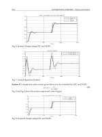
Using Program TRESP in Appendix B to perform a simulation (see Section
3.3) yields the step response for w shown in Figure 3.6.2.
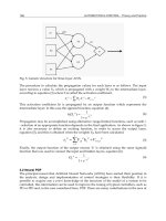
b. Very Flexible Coupling Shaft
Coupling shaft parameters of k=2 N-m/rad and b=0.2 N-m/rad/s correspond
to a very flexible shaft. Using these values, software like PC-MATLAB can be
employed to obtain the two transfer functions
(9)
(10)
Copyright © 2004 by Marcel Dekker, Inc.
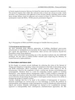
Robot Dynamics160
of approximately 0.1 s due to the flexibility in the shaft.

It is extremely interesting to note that the shaft flexibility has the effect of
speeding up the slowest motor real pole [compare (8) and (9)], so that w
L
approaches its steady-state value more quickly than in the rigid-shaft case.
This is due to the “whipping” action of the flexible shaft.
The shaft dynamics make the control of θ
L
, which corresponds in a robot
arm to the joint angle q
i
, very difficult without some sort of specially designed
controller.
᭿
Figure 3.6.3: Step response of motor with very flexible shaft.
Copyright © 2004 by Marcel Dekker, Inc.
161
3.7 Summary
In this chapter we have laid the foundation for a study of robot control systems.
Using Lagrangian mechanics in Section 3.2, we derived the dynamics of some
robot arms that will be used for demonstration designs throughout the text.
We provided expressions for the general robot arm dynamics for any serial-
link arm.
In Section 3.3 we studied the properties of the robot dynamics such as
boundedness, linearity in the parameters, and skew symmetry that are needed
in controls design. Table 3.3.1 gives a summary of our findings. We used a
Kronecker product approach that yields great insight into the relations between
the terms in the robot equation.
A vital form in modern control systems design is the state-variable
formulation. In Section 3.4 we derived several state-space forms of the arm
dynamics, setting the stage for several design techniques to be provided in

subsequent chapters. The state formulation is also useful in computer simulation
of robot controllers, as we see in Section 3.3.
The dynamics in Cartesian form were given in Section 3.5. The dynamics
of the actuators that drive the robot manipulator links were analyzed and
included in Section 3.6.
3.7 Summary
Copyright © 2004 by Marcel Dekker, Inc.
163
REFERENCES
[Anderson 1989] Anderson, R.J., “Passive computed torque algorithms for robots,”
Proc. IEEE Conf. Decision Control, pp. 1638–1644, Dec. 1989.
[Arimoto and Miyazaki 1984] Arimoto, S., and F.Miyazaki, “Stability and robustness
of PID feedback control for robot manipulators of sensory capability,” Proc.
First Int. Symp., pp. 783–799, MIT, Cambridge, MA, 1984.
[Asada and Slotine 1986] Asada, H., and J J.E.Slotine, Robot Analysis and Control,
New York: Wiley, 1986.
[Borisenko and Tarapov 1968] Borisenko, A.I., and I.E.Tarapov, Vector and Tensor
Analysis with Applications. Englewood Cliffs, NJ: Prentice Hall, 1968.
[Brewer 1978] Brewer, J.W., “Kronecker products and matrix calculus in system
theory,” IEEE Trans. Circuits Syst., vol. CAS-25, no. 9, pp. 772–781, Sept.
1978.
[Craig 1988] Craig, J.J., Adaptive Control of Mechanical Manipulators. Reading,
MA: Addison-Wesley, 1988.
[de Silva 1989] de Silva, C.W., Control Sensors and Actuators. Englewood Cliffs, NJ:
Prentice Hall, 1989.
[Gilbert and Ha 1984] Gilbert, E.G., and I.J.Ha, “An approach to nonlinear feedback
control with applications to robotics,” IEEE Trans. Syst. Man Cybern., vol.
SMC-14, no. 6, pp. 879–884, Nov./Dec. 1984.
[Gu and Loh 1985] Gu, Y L., and N.K.Loh, “Dynamic model for industrial robots
based on a compact Lagrangian formulation,” Proc. IEEE Conf. Decision

Control, pp. 1497–1501, 1985.
[Gu and Loh 1988] Gu, Y-L., and N.K.Loh, “Dynamic modeling and control by
utilizing an imaginary robot model,” IEEE J. Robot. Autom., vol. 4, no. 5, pp.
532–534, Oct. 1988.
Copyright © 2004 by Marcel Dekker, Inc.
165
[Spong and Vidyasagar 1989] Spong, M.W., and M.Vidyasagar, Robot Dynamics
and Control. New York: Wiley, 1989.
[Tarn et al. 1991] Tarn, T J., A.K.Bejczy, X.Yun, and Z.Li, “Effect of motor dynamics
on nonlinear feedback robot arm control,” IEEE Trans. Robot. Autom., vol. 7,
no. 1, pp. 114–122, Feb. 1991.
REFERENCES
Copyright © 2004 by Marcel Dekker, Inc.
166
PROBLEMS
Section 3.2
3.2–1 Dynamics. Find the dynamics for the spherical wrist in Example
A.2–4.
3.2–2 Dynamics from Derived Equations. In Example 3.2.2 we found the
dynamics of the two-link planar elbow arm from first principles. In
this problem, begin with the expressions for the kinetic and potential
energy in that example and:
(a) Write K in the form (3.2.29) to determine M(q).
(b) Use (3.2.42) and (3.2.43) to determine V(q, ) and G(q).
3.2–3 Dynamics from Derived Equations. Repeat Problem 3.2–2 for the
three-link arm in Example 3.2.3.
Section 3.3
3.3–1 Prove (3.3.22) by finding V
p1
(q) and V

v1
(q).
3.3–2 Prove (3.3.23) by finding the matrices V
i
(q).
3.3–3 Prove (3.3.27).
3.3–4 Coriolis Term. Find V
cor
(q) and V
cen
(q) in (3.3.40).
3.3–5 Coriolis Term. Demonstrate that the Coriolis/centripetal term in the
dynamics equation may be expressed [Paul 1981] as V(q, )= vec{V(q,
)}where

with

and T
i
defined in Appendix A. Compare this to V
m1
, V
m2
, V
m
as
defined in Section 3.2.
3.3–6 Bounds and Structure. Derive in detail the results in Example 3.3.1.
REFERENCES
Copyright © 2004 by Marcel Dekker, Inc.

167
3.3–7 Bounds and Structure. Derive the bounds and structural matrices for
the two-link polar arm in Example 3.2.1. Use:
(a) The 1—norm.
(b) The 2-norm .
(c) The ∞—norm.
3.3–8 Bounds and Structure. Repeat Problem 3.3–7 for the three-link
cylindrical arm in Exercise 3.2.3.
3.3–9 Bounds Using 2-Norm. Derive the bounds for the two-link planar
elbow arm in Example 3.3.1 using the 2—norm.
Section 3.4
3.4–1 Prove (3.4.15).
3.4–2 Hamiltonian State Formulation. Demonstrate that (3.4.15) is
equivalent to

with the skew-symmetric matrix defined in Section 3.3.
3.4–3 Hamiltonian State Formulation. Use (3.4.17) to derive the
Hamiltonian state-variable formulation for the two-link polar arm
in Example 3.2.1.
3.4–4 Hamiltonian State Formulation. Repeat Problem 3.4–3 for the two-
link planar elbow arm in Example 3.2.2.
Section 3.5
3.5–1 Cartesian Dynamics. Complete Example 3.5.1, computing the
nonlinear terms in Cartesian coordinates.
3.5–2 Cartesian Dynamics. Find the Cartesian dynamics of the two-link
polar arm in Example 3.2.1.
3.5–3 Cartesian Dynamics. Find the Cartesian dynamics of the two-link
planar elbow arm in Example 3.2.2.
Section 3.6
3.6–1 Actuator Dynamics. Verify that the arm-plus-actuator dynamics (3.6.6)

has the properties listed in Table 3.3.1.
REFERENCES
Copyright © 2004 by Marcel Dekker, Inc.
168
3.6–2 Actuator Dynamics. Derive the third-order dynamics (3.6.12),
providing explicit expressions for Verify that they reduce to
(3.6.5) when L
i
is negligible.
3.6–3 Flexible Coupling Shaft. Verify the state equation for the rigid-shaft
case in Example 3.6.1.
REFERENCES
Copyright © 2004 by Marcel Dekker, Inc.
169
Chapter 4
Computed-Torque Control
In this chapter we examine some straightforward control schemes for robot
manipulators that fall under the class known as “computed-torque controllers.”
These generally perform well when the robot arm parameters are known
fairly accurately. Some connections are given with classical robot control,
and modern design techniques are provided as well. The effects of digital
implementation of robot controllers are shown. Trajectory generation is
outlined.
4.1 Introduction
A basic problem in controlling robots is to make the manipulator follow a
preplanned desired trajectory. Before the robot can do any useful work, we
must position it in the right place at the right instances. In this chapter we
discuss computed-torque control, which yields a family of easy-to-understand
control schemes that often work well in practice. These schemes involve the
decomposition of the controls design problem into an inner-loop design and

an outer-loop design.
In Section 4.4 we provide connections with classical manipulator control
schemes based on independent joint design using PID control. In Section 4.6
we show how to use some modern design techniques in conjunction with
computed-torque control. Thus this chapter could be considered as a bridge
between classical design techniques of the sort used several years ago in robot
control, and the modern design techniques in the remainder of the book which
are needed to obtain high performance in uncertain environments.
We assume here the robot is moving in free space, having no contact with
its environment. Contact results in the generation of forces. The force control
Copyright © 2004 by Marcel Dekker, Inc.
Computed-Torque Control170
problem is dealt with in Chapter 7. We will also assume in this chapter that
the robot is a well-known rigid system, thus designing controllers based on a
fairly well-known model. Control in the presence of uncertainties or unknown
parameters (e.g., friction, payload mass) requires refined approaches. This
problem is dealt with using robust control in Chapter 4 and adaptive control
in Chapter 5.
An actual robot manipulator may have flexibility in its links, or compliance
in its gearing (joint flexibility). In Chapter 6 we cover some aspects of control
with joint flexibility.
Before we can control a robot arm, it is necessary to know the desired path
for performing a task. There are many issues associated with the path planning
problem, such as avoiding obstacles and making sure that the planned path
does not require exceeding the voltage and torque limitations of the actuators.
To reduce the control problem to its basic components, in this chapter we
assume that the ultimate control objective is to move the robot along a
prescribed desired trajectory. We do not concern ourselves with the actual
trajectory-planning problem; we do, however, show how to reconstruct a
continuous desired path from a given table of desired points the end effector

should pass through. This continuous-path generation problem is covered in
Section 4.2.
In most practical situations robot controllers are implemented on
microprocessors, particularly in view of the complex nature of modern control
schemes. Therefore, in Section 4.5 we illustrate some notions of the digital
implementation of robot controllers.
Throughout, we demonstrate how to simulate robot controllers on a
computer. This should be done to verify the effectiveness of any proposed
control scheme prior to actual implementation on a real robot manipulator.
4.2 Path Generation
Throughout the book we assume that there is given a prescribed path q
d
(t) the
robot arm should follow. We design control schemes that make the manipulator
follow this desired path or trajectory. Trajectory planning involves finding
the prescribed path and is usually considered a separate design problem
involving collision avoidance, concerns about actuator saturation, and so on.
See [Lee et al. 1983].
We do not cover trajectory planning. However, we do cover two aspects of
trajectory generation. First, we show how to convert a given prescribed path
from Cartesian space to joint space. Then, given a table of desired points the
end effector should pass through, we show how to reconstruct a continuous
desired trajectory.
Copyright © 2004 by Marcel Dekker, Inc.
171
Converting Cartesian Trajectories to Joint Space
In robotic applications, a desired task is usually specified in the workspace or
Cartesian space, as this is where the motion of the manipulator is easily
described in relation to the external environment and workpiece. However,
trajectory-following control is easily performed in the joint space, as this is

where the arm dynamics are more easily formulated.
Therefore, it is important to be able to find the desired joint space trajectory
q
d
(t) given the desired Cartesian trajectory. This is accomplished using the
inverse kinematics, as shown in the next example. The example illustrates
that the mapping of Cartesian to joint space trajectories may not be unique-
that is, several joint space trajectories may yield the same Cartesian trajectory
for the end-effector.
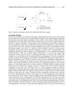
EXAMPLE 4.2–1: Mapping a Prescribed Cartesian Trajectory to Joint
Space
In Example A.3–5 are derived the inverse kinematics for the two-link planar
robot arm shown in Figure 4.2.1. Let us use them to convert a path from
Cartesian space to joint space.
Suppose that we want the two-link arm to follow a given workspace or
Cartesian trajectory
p(t)=(x(t), y(t)) (1)
in the (x, y) plane which is a function of time t. Since the arm is moved by
actuators that control its angles
␪
1
,
␪
2
, it is convenient to convert the specified
Cartesian trajectory (x(t), y(t)) into a joint space trajectory (
␪
1
(t),
␪

2
(t)) for
control purposes.
This may be achieved by using the inverse kinematics transformations
r
2
=x
2
+y
2
(2)
(3)
(4)
␪
2
=ATAN2 (D, C) (5)
4.2 Path Generation
Copyright © 2004 by Marcel Dekker, Inc.
173
Suppose that the end of the arm should repeatedly trace out the circular
workspace path p(t) shown in Figure 4.2.2, which is described by
x(t)=2+½cos t
y(t)=1+½sin t. (7)
By using these expressions for each time t in the inverse kinematics equations,
we obtain the required joint-space trajectories q(t)=(
␪
1
(t),
␪
2

(t)) given in Figure
4.2.3 that yield the circular Cartesian motion of the end effector (using a
1
=2,
a
2
=2).
We have computed the joint variables for the “elbow down” configuration.
Selecting the opposite sign in (4) gives the “elbow up” joint space trajectory
yielding the same Cartesian trajectory.
Polynomial Path Interpolation
Suppose that a desired trajectory for the manipulator motion has been
determined, either in Cartesian space or, using the inverse kinematics, in joint
space. For convenience, we use the joint space variable q(t) for notation. It is
not possible to store the entire trajectory in computer memory, and few
practically useful trajectories have a simple closed-form expression. Therefore,
it is usual to store in computer memory a sequence of points q
i
(t
k
) for each
joint variable i that represent the desired values of that variable at the discrete
times t
k
. Thus q(t
k
) is a point in R
n
that the joint variables should pass through
at time t

k
.We call these via points.
Most robot control schemes require a continuous desired trajectory. To
convert the table of via points q
i
(t
k
) to a continuous desired trajectory q
d
(t), we
may use many options. Let us discuss here polynomial interpolation.
Suppose that the via points are uniformly spaced in time and define the
sampling period as
T=t
k+1
-t
k
. (4.2.1)
For smooth motion, on each time interval [t
k
, t
k+1
] we require the desired
position q
d
(t) and velocity q
.
d
(t) to match the tabulated via points. This yields
boundary conditions of

᭿
4.2 Path Generation
Copyright © 2004 by Marcel Dekker, Inc.