The MEMS Handbook (1st Ed) - M. Gad el Hak Part 2 ppt
Bạn đang xem bản rút gọn của tài liệu. Xem và tải ngay bản đầy đủ của tài liệu tại đây (121.41 KB, 4 trang )
© 2002 by CRC Press LLC
4.7 Molecular-Based Models
In the continuum models discussed thus far, the macroscopic fluid properties are the dependent variables,
while the independent variables are the three spatial coordinates and time. The molecular models recognize
the fluid as a myriad of discrete particles: molecules, atoms, ions and electrons. The goal here is to
determine the position, velocity and state of all particles at all times. The molecular approach is either
deterministic or probabilistic (refer to Figure 4.1). Provided that there is a sufficient number of micro-
scopic particles within the smallest significant volume of a flow, the macroscopic properties at any location
in the flow can then be computed from the discrete-particle information by a suitable averaging or
weighted averaging process. This section discusses molecular-based models and their relation to the
continuum models previously considered.
The most fundamental of the molecular models is a deterministic one. The motion of the molecules
is governed by the laws of classical mechanics, although, at the expense of greatly complicating the
problem, the laws of quantum mechanics can also be considered in special circumstances. The modern
molecular dynamics (MD) computer simulations have been pioneered by Alder and Wainwright (1957;
1958; 1970) and reviewed by Ciccotti and Hoover (1986), Allen and Tildesley (1987), Haile (1993) and
Koplik and Banavar (1995). The simulation begins with a set of N molecules in a region of space, each
assigned a random velocity corresponding to a Boltzmann distribution at the temperature of interest.
The interaction between the particles is prescribed typically in the form of a two-body potential energy,
and the time evolution of the molecular positions is determined by integrating Newton’s equations of
motion. Because MD is based on the most basic set of equations, it is valid in principle for any flow
extent and any range of parameters. The method is straightforward in principle but has two hurdles:
choosing a proper and convenient potential for particular fluid and solid combinations and the colossal
computer resources required to simulate a reasonable flowfield extent.
For purists, the former difficulty is a sticky one. There is no totally rational methodology by which a
convenient potential can be chosen. Part of the art of MD is to pick an appropriate potential and validate
the simulation results with experiments or other analytical/computational results. A commonly used
potential between two molecules is the generalized Lennard–Jones 6–12 potential, to be used in the
following section and further discussed in the section following that.
The second difficulty, and by far the most serious limitation of molecular dynamics simulations, is
the number of molecules N that can realistically be modeled on a digital computer. Because the compu-
tation of an element of trajectory for any particular molecule requires consideration of all other molecules
as potential collision partners, the amount of computation required by the MD method is proportional
to N
2
. Some saving in computer time can be achieved by cutting off the weak tail of the potential (see
Figure 4.11) at, say, r
c
= 2.5 σ and shifting the potential by a linear term in r so that the force goes smoothly
to zero at the cutoff. As a result, only nearby molecules are treated as potential collision partners, and
the computation time for N molecules no longer scales with N
2
.
The state of the art of molecular dynamics simulations in the early 2000s is such that with a few hours
of CPU time general-purpose supercomputers can handle around 100,000 molecules. At enormous
expense, the fastest parallel machine available can simulate around 10 million particles. Because of the
extreme diminution of molecular scales, the above translates into regions of liquid flow of about 0.02
µm
(200 Å) in linear size, over time intervals of around 0.001
µs, enough for continuum behavior to set in
for simple molecules. To simulate 1 s of real time for complex molecular interactions (e.g., including
vibration modes, reorientation of polymer molecules, collision of colloidal particles) requires unrealistic
CPU time measured in hundreds of years.
Molecular dynamics simulations are highly inefficient for dilute gases where the molecular interac-
tions are infrequent. The simulations are more suited for dense gases and liquids. Clearly, molecular
dynamics simulations are reserved for situations where the continuum approach or the statistical
methods are inadequate to compute from first principles important flow quantities. Slip-boundary
conditions for liquid flows in extremely small devices are such a case, as will be discussed in the following
section.
© 2002 by CRC Press LLC
5
Integrated Simulation
for MEMS: Coupling
Flow-Structure-
Thermal-Electrical
Domains
5.1 Abstract
5.2 Introduction
Full-System Simulation • Computational Complexity of
MEMS Flows • Coupled-Domain Problems • A Prototype
Problem
5.3 Coupled Circuit-Device Simulation
5.4 Overview of Simulators
The Circuit Simulator: SPICE3 • The Fluid Simulator:
N
εκ
T
α
r
• Formulation for Flow-Structure
Interactions • Grid Velocity Algorithm • The Structural
Simulator • Differences between Circuit, Fluid and Solid
Simulators
5.5 Circuit-Microfluidic Device Simulation
Software Integration • Lumped Element and Compact Models
for Devices
5.6 Demonstrations of the Integrated
Simulation Approach
Microfluidic System Description • SPICE3–
N
εκ
T
α
r
Integration • Simulation Results
5.7 Summary and Discussion
Acknowledgments
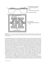
5.1 Abstract
Full-system simulation of microelectromechanical systems (MEMS) involves coupling of many diverse pro-
cesses with disparate spatial and temporal scales. In its simplest form, all elements in a MEMS device are
represented as equivalent analog circuits so that robust simulators such as SPICE can solve for the entire
system. However, devices, and especially fluidic devices, do not usually have such equivalent analogs and
may require full simulation of individual components. This is particularly true for new designs, which
often involve unfamiliar physics; such lumped models and continuum approximations are inappropriate
in this case. In this chapter, we address such issues for an integrated simulation approach for MEMS with
Robert M. Kirby
Brown University
George Em Karniadakis
Brown University
Oleg Mikulchenko
Oregon State University
Kartikeya Mayaram
Oregon State University
© 2002 by CRC Press LLC
6
Liquid Flows in
Microchannels
6.1 Introduction
Unique Aspects of Liquids in Microchannels • Continuum
Hydrodynamics of Pressure Driven Flow in
Channels • Hydraulic Diameter • Flow in Round
Capillaries • Entrance Length Development • Transition to
Turbulent Flow • Noncircular Channels
6.2 Experimental Studies of Flow
Through Microchannels
Proposed Explanations for Measured
Behavior • Measurements of Velocity in
Microchannels • Nonlinear Channels • Capacitive Effects
6.3 Electrokinetics Background
Electrical Double Layers • EOF with Finite EDL • Thin EDL
Electro-Osmotic Flow • Electrophoresis • Similarity
between Electric and Velocity Fields for Electro-Osmosis and
Electrophoresis • Electrokinetic Microchips • Engineering
Considerations: Flowrate and Pressure of Electro-Osmotic
Flow • Electrical Analogy and Microfluidic
Networks • Practical Considerations
6.4 Summary and Conclusions
Nomenclature
6.1 Introduction
Nominally, microchannels can be defined as channels whose dimensions are less than 1 mm and greater
than 1
µ
m. Above 1 mm the flow exhibits behavior that is the same as most macroscopic flows. Below
1
µ
m the flow is better characterized as nanoscopic. Currently, most microchannels fall into the range
of 30 to 300
µ
m. Microchannels can be fabricated in many materials—glass, polymers, silicon, metals—
using various processes including surface micromachining, bulk micromachining, molding, embossing
and conventional machining with microcutters. These methods and the characteristics of the resulting
flow channels are discussed elsewhere in this handbook.
Microchannels offer advantages due to their high surface-to-volume ratio and their small volumes.
The large surface-to-volume ratio leads to a high rate of heat and mass transfer, making microdevices
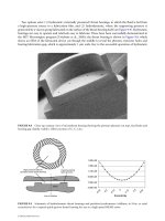
excellent tools for compact heat exchangers. For example, the device in Figure 6.1 is a cross-flow heat
exchanger constructed from a stack of 50 14-mm
×
14-mm foils, each containing 34 200-
µ
m-wide
×
100-
µ
m-deep channels machined into the 200-
µ
m-thick stainless steel foils by the process of direct,
high-precision mechanical micromachining [Brandner et al., 2000; Schaller et al., 1999]. The direction
of flow in adjacent foils is alternated 90
°
, and the foils are attached by means of diffusion bonding to
create a stack of cross-flow heat exchangers capable of transferring 10 kW at a temperature difference of
Kendra V. Sharp
University of Illinois at
Urbana–Champaign
Ronald J. Adrian
University of Illinois at
Urbana–Champaign
Juan G. Santiago
Stanford University
Joshua I. Molho
Stanford University