The MEMS Handbook Introduction & Fundamentals (2nd Ed) - M. Gad el Hak Part 3 pptx
Bạn đang xem bản rút gọn của tài liệu. Xem và tải ngay bản đầy đủ của tài liệu tại đây (359.56 KB, 30 trang )
In boundary layers, the relevant length scale is the shear-layer thickness
δ
, and for laminar flows
ϳ (4.9)
Kn ϳ ϳ (4.10)
where Re
δ
is the Reynolds number based on the freestream velocity v
o
, and the boundary layer thickness
δ
, and Re is based on v
o
and the streamwise length scale L.
Rarefied gas flows are in general encountered in flows in small geometries, such as MEMS devices, and
in low-pressure applications, such as high-altitude flying and high-vacuum gadgets. The local value of
Knudsen number in a particular flow determines the degree of rarefaction and the degree of validity of
the Navier–Stokes model. The different Knudsen number regimes are determined empirically and are
therefore only approximate for a particular flow geometry. The pioneering experiments in rarefied gas
dynamics were conducted by Knudsen in 1909. In the limit of zero Knudsen number, the transport terms
in the continuum momentum and energy equations are negligible, and the Navier–Stokes equations then
reduce to the inviscid Euler equations. Both heat conduction and viscous diffusion and dissipation are
negligible, and the flow is then approximately isentropic (i.e., adiabatic and reversible) from the contin-
uum viewpoint, while the equivalent molecular viewpoint is that the velocity distribution function is
everywhere of the local equilibrium or Maxwellian form. As Kn increases, rarefaction effects become
more important, and eventually the continuum approach breaks down altogether. The different Knudsen
number regimes are depicted in Figure 4.2, and can be summarized as follows:
Euler equations (neglect molecular diffusion): Kn → 0 (Re
→
∞)
Navier–Stokes equations with no-slip boundary conditions: Kn Ͻ 10
–3
Navier–Stokes equations with slip boundary conditions: 10
–3
р Kn Ͻ 10
–1
Transition regime: 10
–1
р Kn Ͻ 10
Free-molecule flow: Kn у 10
As an example, consider air at standard temperature (T ϭ 288 K) and pressure (p ϭ 1.01 ϫ10
5
N/m
2
).
A cube one micron on a side contains 2.54 ϫ 10
7
molecules separated by an average distance of
0.0034 microns. The gas is considered dilute if the ratio of this distance to the molecular diameter exceeds
7; in the present example this ratio is 9, barely satisfying the dilute gas assumption. The mean free path
computed from Equation (4.1) is L ϭ 0.065 µm. A microdevice with characteristic length of 1 µm would
have Kn ϭ 0.065, which is in the slip-flow regime. At lower pressures, the Knudsen number increases. For
example, if the pressure is 0.1 atm and the temperature remains the same, Kn ϭ 0.65 for the same 1 µm
Ma
ᎏ
͙
R
ෆ
e
ෆ
Ma
ᎏ
Re
δ
1
ᎏ
͙
R
ෆ
e
ෆ
δ
ᎏ
L
Flow Physics 4-5
Kn = 0.0001 0.001 0.01 0.1 1 10010
Continuum flow
(ordinary density levels)
(slightly rarefied)
Slip-flow regime
Transition regime
Free-molecule flow
(moderately rarefied)
(highly rarefied)
FIGURE 4.2 Knudsen number regimes.
© 2006 by Taylor & Francis Group, LLC
device, and the flow is then in the transition regime. There would still be more than 2 million molecules
in the same 1 µm cube, and the average distance between them would be 0.0074 µm. The same device at
100 km altitude would have Kn ϭ 3 ϫ 10
4
,well into the free-molecule flow regime. Knudsen number for
the flow of a light gas like helium is about three times larger than that for air flow at otherwise the same
conditions.
Consider a long microchannel where the entrance pressure is atmospheric and the exit conditions are
near vacuum. As air goes down the duct, the pressure and density decrease while the velocity, Mach num-
ber, and Knudsen number increase. The pressure drops to overcome viscous forces in the channel. If
isothermal conditions prevail,
1
density also drops and conservation of mass requires the flow to acceler-
ate down the constant-area tube. The fluid acceleration in turn affects the pressure gradient resulting in
a nonlinear pressure drop along the channel. The Mach number increases down the tube, limited only by
choked-flow condition Ma ϭ 1. Additionally, the normal component of velocity is no longer zero. With
lower density, the mean free path increases, and Kn correspondingly increases. All flow regimes depicted
in Figure 4.2 may occur in the same tube: continuum with no-slip boundary conditions, slip-flow regime,
transition regime, and free-molecule flow. The air flow may also change from incompressible to com-
pressible as it moves down the microduct. A similar scenario may take place if the entrance pressure is,
say, 5atm, while the exit is atmospheric. This deceivingly simple duct flow may in fact manifest every single
complexity discussed in this section. The following six sections discuss in turn the Navier–Stokes equa-
tions, compressibility effects, boundary conditions, molecular-based models, liquid flows, and surface
phenomena.
4.4 Navier–Stokes Equations
This section recalls the traditional conservation relations in fluid mechanics. A concise derivation of these
equations can be found in Gad-el-Hak (2000). Here, we reemphasize the precise assumptions needed to
obtain a particular form of the equations. A continuum fluid implies that the derivatives of all the
dependent variables exist in some reasonable sense. In other words, local properties, such as density and
velocity, are defined as averages over elements that are large compared with the microscopic structure of
the fluid but small enough in comparison with the scale of the macroscopic phenomena to permit the use
of differential calculus to describe them. As mentioned earlier, such conditions are almost always met. For
such fluids, and assuming the laws of nonrelativistic mechanics hold, the conservation of mass, momen-
tum, and energy can be expressed at every point in space and time as a set of partial differential equations
as follows:
ϩ (
ρ
u
k
) ϭ 0
(4.11)
ρ
ϩ
u
k
ϭ ϩ
ρ
g
i
(4.12)
ρ
ϩ u
k
ϭ Ϫ ϩ Σ
ki
(4.13)
where
ρ
is the fluid density, u
k
is an instantaneous velocity component (u, v, w), Σ
ki
is the second-order
stress tensor (surface force per unit area), g
i
is the body force per unit mass, e is the internal energy, and
q
k
is the sum of heat flux vectors due to conduction and radiation. The independent variables are time t
and the three spatial coordinates x
1
, x
2
, and x
3
or (x, y, z).
∂u
i
ᎏ
∂x
k
∂q
k
ᎏ
∂x
k
∂e
ᎏ
∂x
k
∂e
ᎏ
∂t
∂Σ
ki
ᎏ
∂x
k
∂u
i
ᎏ
∂x
k
∂u
i
ᎏ
∂t
∂
ᎏ
∂x
k
∂
ρ
ᎏ
∂t
4-6 MEMS: Introduction and Fundamentals
1
More likely the flow will be somewhere between isothermal and adiabatic, Fanno flow. In that case both density
and temperature decrease downstream, the former not as fast as in the isothermal case. None of that changes the qual-
itative arguments made in the example.
© 2006 by Taylor & Francis Group, LLC
Equations (4.11), (4.12), and (4.13) constitute five differential equations for the 17 unknowns
ρ
, u
i
, Σ
ki
,
e, and q
k
. Absent any body couples, the stress tensor is symmetric having only six independent compo-
nents, which reduces the number of unknowns to 14. Obviously, the continuum flow equations do not
form a determinate set. To close the conservation equations, the relation between the stress tensor and
deformation rate, the relation between the heat flux vector and the temperature field, and appropriate
equations of state relating the different thermodynamic properties are needed. The stress–rate-of-strain
relation and the heat-flux–temperature-gradient relation are approximately linear if the flow is not too
far from thermodynamic equilibrium. This is a phenomenological result but can be rigorously derived
from the Boltzmann equation for a dilute gas assuming the flow is near equilibrium. For a Newtonian,
isotropic, Fourier, ideal gas, for example, those relations read
Σ
ki
ϭ Ϫp
δ
ki
ϩ
µ
ϩ
ϩ
λ
δ
ki
(4.14)
q
i
ϭ Ϫ
κ
ϩ Heat flux due to radiation (4.15)
de ϭ c
v
dT and p ϭ
ρ
T (4.16)
where p is the thermodynamic pressure,
µ
and
λ
are the first and second coefficients of viscosity, respectively,
δ
ki
is the unit second-order tensor (Kronecker delta),
κ
is the thermal conductivity, T is the temperature
field, c
v
is the specific heat at constant volume, and
is the gas constant which is given by the Boltzmann
constant divided by the mass of an individual molecule k ϭ m
. Stokes’ hypothesis relates the first and
second coefficients of viscosity thus,
λ
ϩ
ᎏ
2
3
ᎏ
µ
ϭ 0, although the validity of this assumption for other than
dilute, monatomic gases has occasionally been questioned [Gad-el-Hak, 1995]. With the above constitu-
tive relations and neglecting radiative heat transfer, Equations (4.11), (4.12), and (4.13) respectively read
ϩ (
ρ
u
k
) ϭ 0 (4.17)
ρ
ϩ u
k
ϭ Ϫ ϩ
ρ
g
i
ϩ
΄
µ
ϩ
ϩ
δ
k
i
λ
΅
(4.18)
ρ
ϩ u
k
ϭ
κ
Ϫ
p
ϩ
φ
(4.19)
The three components of the vector Equation (4.18) are the Navier–Stokes equations expressing the con-
servation of momentum for a Newtonian fluid. In the thermal energy Equation (4.19),
φ
is the always
positive dissipation function expressing the irreversible conversion of mechanical energy to internal
energy as a result of the deformation of a fluid element. The second term on the right-hand side of (4.19)
is the reversible work done (per unit time) by the pressure as the volume of a fluid material element
changes. For a Newtonian, isotropic fluid, the viscous dissipation rate is given by
φ
ϭ
µ
ϩ
2
ϩ
λ
2
(4.20)
There are now six unknowns,
ρ
, u
i
, p, and T, and the five coupled Equations (4.17), (4.18), and (4.19) plus
the equation of state relating pressure, density, and temperature. These six equations together with suffi-
cient number of initial and boundary conditions constitute a well-posed, albeit formidable, problem. The
system of Equations (4.17)–(4.19) is an excellent model for the laminar or turbulent flow of most fluids,
such as air and water, under many circumstances including high-speed gas flows for which the shock
waves are thick relative to the mean free path of the molecules.
∂u
j
ᎏ
∂x
j
∂u
k
ᎏ
∂x
i
∂u
i
ᎏ
∂x
k
1
ᎏ
2
∂u
k
ᎏ
∂x
k
∂T
ᎏ
∂x
k
∂
ᎏ
∂x
k
∂e
ᎏ
∂x
k
∂e
ᎏ
∂t
∂u
j
ᎏ
∂x
j
∂u
k
ᎏ
∂x
i
∂u
i
ᎏ
∂x
k
∂
ᎏ
∂x
k
∂
ρ
ᎏ
∂x
i
∂u
i
ᎏ
∂x
k
∂u
i
ᎏ
∂t
∂
ᎏ
∂x
k
∂
ρ
ᎏ
∂t
∂T
ᎏ
∂x
i
∂u
j
ᎏ
∂x
j
∂u
k
ᎏ
∂x
i
∂u
i
ᎏ
∂x
k
Flow Physics 4-7
© 2006 by Taylor & Francis Group, LLC
Considerable simplification is achieved if the flow is assumed incompressible, usually a reasonable
assumption provided that the characteristic flow speed is less than 0.3 of the speed of sound. The incom-
pressibility assumption is readily satisfied for almost all liquid flows and many gas flows. In such cases,
the density is assumed either a constant or a given function of temperature (or species concentration).
The governing equations for such flow are
ϭ 0 (4.21)
ρ
ϩ
u
k
ϭ Ϫ ϩ
΄
µ
ϩ
΅
ϩ
ρ
gi (4.22)
ρ
c
p
ϩ
u
k
ϭ
κ
ϩ
φ
incomp
(4.23)
where
φ
incomp
is the incompressible limit of Equation (4.20). These are now five equations for the five
dependent variables u
i
, p, and T. Note that the left-hand side of Equation (4.23) has the specific heat at
constant pressure c
p
and not c
v
. It is the convection of enthalpy — and not internal energy — that is balanced
by heat conduction and viscous dissipation. This is the correct incompressible-flow limit — of a compressi-
ble fluid — as discussed in detail in Section 10.9 of Panton (1996); a subtle point, perhaps, but one that
is frequently missed in textbooks.
For both the compressible and the incompressible equations of motion, the transport terms are neg-
lected away from solid walls in the limit of infinite Reynolds number (Kn → 0). The fluid is then approx-
imated as inviscid and nonconducting, and the corresponding equations read (for the compressible case)
ϩ (
ρ
u
k
) ϭ 0 (4.24)
ρ
ϩ
u
k
ϭ Ϫ ϩ
ρ
g
i
(4.25)
ρ
c
v
ϩ
u
k
ϭ Ϫp (4.26)
The Euler Equation (4.25) can be integrated along a streamline, and the resulting Bernoulli’s equation
provides a direct relation between the velocity and pressure.
4.5 Compressibility
The issue of whether to consider the continuum flow compressible or incompressible seems straightfor-
ward but is in fact full of potential pitfalls. If the local Mach number is less than 0.3, then the flow of a
compressible fluid like air can — according to the conventional wisdom — be treated as incompressible.
But the well-known Ma Ͻ 0.3 criterion is only a necessary criterion, not a sufficient one, to allow a treat-
ment of the flow as approximately incompressible. In other words, in some situations the Mach number
can be exceedingly small while the flow is compressible. As is well documented in heat transfer textbooks,
strong wall heating or cooling may cause the density to change sufficiently and the incompressible
approximation to break down, even at low speeds. Less known is the situation encountered in some
microdevices where the pressure may strongly change due to viscous effects even though the speeds may
not be high enough for the Mach number to go above the traditional threshold of 0.3. Corresponding to
the pressure changes would be strong density changes that must be taken into account when writing the
continuum equations of motion. In this section, we systematically explain all situations where compress-
ibility effects must be considered. Let us rewrite the full continuity Equation (4.11) as follows
ϩ
ρ
ϭ 0 (4.27)
∂u
k
ᎏ
∂x
k
D
ρ
ᎏ
Dt
∂u
k
ᎏ
∂x
k
∂T
ᎏ
∂x
k
∂T
ᎏ
∂t
∂p
ᎏ
∂x
i
∂u
i
ᎏ
∂x
k
∂u
i
ᎏ
∂t
∂
ᎏ
∂x
k
∂
ρ
ᎏ
∂t
∂T
ᎏ
∂x
k
∂
ᎏ
∂x
k
∂T
ᎏ
∂x
k
∂T
ᎏ
∂t
∂u
k
ᎏ
∂x
i
∂u
i
ᎏ
∂x
k
∂
ᎏ
∂x
k
∂p
ᎏ
∂x
i
∂u
i
ᎏ
∂x
k
∂u
i
ᎏ
∂t
∂u
k
ᎏ
∂x
k
4-8 MEMS: Introduction and Fundamentals
© 2006 by Taylor & Francis Group, LLC
where
is the substantial derivative
ϩ u
k
expressing changes following a fluid element. The proper criterion for the incompressible approximation
to hold is that
is vanishingly small. In other words, if density changes following a fluid particle are small, the flow is
approximately incompressible. Density may change arbitrarily from one particle to another without vio-
lating the incompressible flow assumption. This is the case, for example, in the stratified atmosphere and
ocean, where the variable-density/temperature/salinity flow is often treated as incompressible.
From the state principle of thermodynamics, we can express the density changes of a simple system in
terms of changes in pressure and temperature,
ρ
ϭ
ρ
(p, T) (4.28)
Using the chain rule of calculus,
ϭ
α
Ϫ
β
(4.29)
where
α
and
β
are respectively the isothermal compressibility coefficient and the bulk expansion coeffi-
cient — two thermodynamic variables that characterize the fluid susceptibility to change of volume —
which are defined by the following relations
α
(p, T) ≡
Έ
T
(4.30)
β
(p, T) ≡ Ϫ
Έ
p
(4.31)
For ideal gases,
α
ϭ 1/p and
β
ϭ 1/T. Note, however, that in the following arguments invoking the ideal
gas assumption will not be necessary. The flow must be treated as compressible if pressure- and/or
temperature-changes — following a fluid element — are sufficiently strong. Equation (4.29) must, of
course, be properly nondimensionalized before deciding whether a term is large or small. Here, we follow
closely the procedure detailed in Panton (1996).
Consider first the case of adiabatic walls. Density is normalized with a reference value
ρ
o
, velocities
with a reference speed v
o
, spatial coordinates and time with respectively L and L/v
o
, the isothermal com-
pressibility coefficient and bulk expansion coefficient with reference values
α
o
and
β
o
. The pressure is
nondimensionalized with the inertial pressure-scale
ρ
o
v
2
o
. This scale is twice the dynamic pressure; that is,
the pressure change as an inviscid fluid moving at the reference speed is brought to rest.
Temperature changes for adiabatic walls can only result from the irreversible conversion of mechanical
energy into internal energy via viscous dissipation. Temperature is therefore nondimensionalized as follows
T
*
ϭ
T Ϫ T
o
ϭ
T Ϫ T
o
Pr
(4.32
)
where T
o
is a reference temperature,
µ
o
,
κ
o
, and c
p
o
are respectively reference viscosity, thermal, conductiv-
ity, and specific heat at constant pressure, and Pr is the reference Prandtl number, (
µ
o
c
p
o
)/
κ
o
.
v
2
o
ᎏ
c
p
o
µ
o
v
2
o
ᎏ
c
κ
o
∂
ρ
ᎏ
∂T
1
ᎏ
ρ
∂
ρ
ᎏ
∂p
1
ᎏ
ρ
DT
ᎏ
Dt
Dp
ᎏ
Dt
D
ρ
ᎏ
Dt
1
ᎏ
ρ
D
ρ
ᎏ
Dt
1
ᎏ
ρ
∂
ᎏ
∂x
k
∂
ᎏ
∂t
D
ᎏ
Dt
Flow Physics 4-9
© 2006 by Taylor & Francis Group, LLC
In the present formulation, the scaling used for pressure is based on the Bernoulli’s equation and there-
fore neglects viscous effects. This particular scaling guarantees that the pressure term in the momentum
equation will be of the same order as the inertia term. The temperature scaling assumes that the conduc-
tion, convection, and dissipation terms in the energy equation have the same order of magnitude. The
resulting dimensionless form of Equation (4.29) reads
ϭ
γ
o
Ma
2
Ά
α
* Ϫ
·
(4.33)
where the superscript * indicates a nondimensional quantity, Ma is the reference Mach number (v
o
/a
o
,
where a
o
is the reference speed of sound), and A and B are dimensionless constants defined by A ≡
α
o
ρ
o
c
p
o
T
o
and B ≡
β
o
T
o
. If the scaling is properly chosen, the terms having the * superscript in the right-hand side
should be of order one, and the relative importance of such terms in the equations of motion is deter-
mined by the magnitude of the dimensionless parameters appearing to their left (e.g. Ma, Pr, etc.).
Therefore, as Ma
2
→ 0, temperature changes due to viscous dissipation are neglected (unless Pr is very
large as, for example, in the case of highly viscous polymers and oils). Within the same order of approx-
imation, all thermodynamic properties of the fluid are assumed constant.
Pressure changes are also neglected in the limit of zero Mach number. Hence, for Ma Ͻ 0.3 (i.e.,
Ma
2
Ͻ 0.09), density changes following a fluid particle can be neglected and the flow can then be approx-
imated as incompressible.
2
However, there is a caveat to this argument. Pressure changes due to inertia
can indeed be neglected at small Mach numbers, and this is consistent with the way we nondimensional-
ized the pressure term above. If, on the other hand, pressure changes are mostly due to viscous effects, as
is the case, for example, in a long microduct or a micro-gas-bearing, pressure changes may be significant
even at low speeds (low Ma). In that case the term
in Equation (4.33) is no longer of order one and may be large regardless of the value of Ma. Density then
may change significantly, and the flow must be treated as compressible. Had pressure been nondimen-
sionalized using the viscous scale
instead of the inertial one
(
ρ
o
v
2
o
)
the revised Equation (4.33) would have Re
Ϫ1
appearing explicitly in the first term in the right-hand side,
accentuating this term’s importance when viscous forces dominate.
A similar result can be gleaned when the Mach number is interpreted as follows
Ma
2
ϭ ϭ v
2
o
Έ
s
ϭ
Έ
s
ϳ
ϭ (4.34)
where s is the entropy. Again, the above equation assumes that pressure changes are inviscid, and there-
fore small Mach number means negligible pressure and density changes. In a flow dominated by viscous
effects — such as that inside a microduct — density changes may be significant even in the limit of zero
Mach number.
Identical arguments can be made in the case of isothermal walls. Here strong temperature changes
may be the result of wall heating or cooling even if viscous dissipation is negligible. The proper
∆
ρ
ᎏ
ρ
o
∆
ρ
ᎏ
∆p
∆p
ᎏ
ρ
o
∂
ρ
ᎏ
∂p
ρ
o
v
2
o
ᎏ
ρ
o
∂
ρ
ᎏ
∂p
v
2
o
ᎏ
a
2
o
µ
o
v
o
ᎏ
L
Dp*
ᎏ
Dt
DT*
ᎏ
Dt
*
PrB
β
*
ᎏ
A
Dp*
ᎏ
Dt
*
D
ρ
*
ᎏ
Dt
*
1
ᎏ
ρ
*
4-10 MEMS: Introduction and Fundamentals
2
With an error of about 10% at Ma ϭ 0.3, 4% at Ma ϭ 0.2, 1% at Ma ϭ 0.1, and so on.
© 2006 by Taylor & Francis Group, LLC
temperature scale in this case is given in terms of the wall temperature T
w
and the reference temperature
T
o
as follows
T ϭ (4.35)
where
T is the new dimensionless temperature. The nondimensional form of Equation (4.29) now reads
ϭ
γ
o
Ma
2
α
*
Ϫ
β
*
B
(4.36)
Here we notice that the temperature term is different from that in Equation (4.33). Ma no longer appears
in this term, and strong temperature changes, that is, large (T
w
Ϫ T
o
)/T
o
, may cause strong density
changes regardless of the value of the Mach number. Additionally, the thermodynamic properties of the
fluid are not constant but depend on temperature; as a result the continuity, momentum, and energy
equations all couple. The pressure term in Equation (4.36), on the other hand, is exactly as it was in the
adiabatic case, and the arguments made before apply: the flow should be considered compressible if
Ma Ͼ 0.3 or if pressure changes due to viscous forces are sufficiently large.
Experiments in gaseous microducts confirm the above arguments. For both low- and high-Mach-
number flows, pressure gradients in long microchannels are nonconstant, consistent with the compress-
ible flow equations. Such experiments were conducted by, among others, Prud’homme et al. (1986),
Pfahler et al. (1991), van den Berg et al. (1993), Liu et al. (1993, 1995), Pong et al. (1994), Harley et al.
(1995), Piekos and Breuer (1996), Arkilic (1997), and Arkilic et al. (1995, 1997a, 1997b). Sample results
will be presented in the following section.
In three additional scenarios significant pressure and density changes may take place without inertial,
viscous, or thermal effects. First is the case of quasi-static compression/expansion of a gas in, for exam-
ple, a piston-cylinder arrangement. The resulting compressibility effects are, however, compressibility of
the fluid and not of the flow. Two other situations where compressibility effects must also be considered
are problems with length-scales comparable to the scale height of the atmosphere and rapidly varying
flows as in sound propagation [Lighthill, 1963].
4.6 Boundary Conditions
The continuum equations of motion described earlier require a certain number of initial and boundary
conditions for proper mathematical formulation of flow problems. In this section, we describe the
boundary conditions at a fluid–solid interface. Boundary conditions in the inviscid flow theory pertain
only to the velocity component normal to a solid surface. The highest spatial derivative of velocity in the
inviscid equations of motion is first order, and only one velocity boundary condition at the surface is
admissible. The normal velocity component at a fluid–solid interface is specified, and no statement can
be made regarding the tangential velocity component. The normal-velocity condition simply states that
a fluid-particle path cannot go through an impermeable wall. Real fluids are viscous, of course, and the
corresponding momentum equation has second-order derivatives of velocity, thus requiring an addi-
tional boundary condition on the velocity component tangential to a solid surface.
Traditionally, the no-slip condition at a fluid–solid interface is enforced in the momentum equation,
and an analogous no-temperature-jump condition is applied in the energy equation. The notion under-
lying the no-slip/no-jump condition is that within the fluid there cannot be any finite discontinuities of
velocity/temperature. Those would involve infinite velocity/temperature gradients and so produce infi-
nite viscous stress/heat flux that would destroy the discontinuity in infinitesimal time. The interaction
between a fluid particle and a wall is similar to that between neighboring fluid particles, and therefore no
discontinuities are allowed at the fluid–solid interface either. In other words, the fluid velocity must be zero
relative to the surface, and the fluid temperature must be equal to that of the surface. But strictly speak-
ing those two boundary conditions are valid only if the fluid flow adjacent to the surface is in thermody-
namic equilibrium. This requires an infinitely high frequency of collisions between the fluid and the solid
surface. In practice, the no-slip/no-jump condition leads to fairly accurate predictions as long as
D
T
ᎏ
Dt
*
T
w
Ϫ T
o
ᎏ
T
o
Dp
*
ᎏ
Dt
*
D
ρ
*
ᎏ
Dt
*
1
ᎏ
ρ
*
T Ϫ T
o
ᎏ
T
w
Ϫ T
o
Flow Physics 4-11
© 2006 by Taylor & Francis Group, LLC
Kn Ͻ 0.001 (for gases). Beyond that, the collision frequency is simply not high enough to ensure equilib-
rium, and a certain degree of tangential-velocity slip and temperature jump must be allowed. This is a
case frequently encountered in MEMS flows, and we develop the appropriate relations in this section.
For both liquids and gases, the linear Navier boundary condition empirically relates the tangential
velocity slip at the wall ∆u|
w
to the local shear
∆u|
w
ϭ u
fluid
Ϫ u
wall
ϭ L
s
Έ
w
(4.37)
where L
s
is the constant slip length, and
Έ
w
is the strain rate computed at the wall. In most practical situations, the slip length is so small that the
no-slip condition holds. In MEMS applications, however, that may not be the case. Once again we defer
the discussion of liquids to a later section and focus for now on gases.
Assuming isothermal conditions prevail, the above slip relation has been rigorously derived by
Maxwell (1879) from considerations of the kinetic theory of dilute, monatomic gases. Gas molecules,
modeled as rigid spheres, continuously strike and reflect from a solid surface, just as they continuously
collide with each other. For an idealized perfectly smooth wall (at the molecular scale), the incident angle
exactly equals the reflected angle, and the molecules conserve their tangential momentum and thus exert
no shear on the wall. This is termed specular reflection and results in perfect slip at the wall. For an
extremely rough wall, on the other hand, the molecules reflect at some random angle uncorrelated with
their entry angle. This perfectly diffuse reflection results in zero tangential-momentum for the reflected
fluid molecules to be balanced by a finite slip velocity in order to account for the shear stress transmitted
to the wall. A force balance near the wall leads to the following expression for the slip velocity
u
gas
Ϫ u
wall
ϭ L
Έ
w
(4.38)
where L is the mean free path. The right-hand side can be considered as the first term in an infinite Taylor
series, sufficient if the mean free path is relatively small enough. Equation (4.38) states that significant slip
occurs only if the mean velocity of the molecules varies appreciably over a distance of one mean free path.
This is the case, for example, in vacuum applications and/or flow in microdevices. The number of colli-
sions between the fluid molecules and the solid in those cases is not large enough for even an approxi-
mate flow equilibrium to be established. Furthermore, additional (nonlinear) terms in the Taylor series
would be needed as L increases and the flow is further removed from the equilibrium state.
For real walls some molecules reflect diffusively and some reflect specularly. In other words, a portion of
the momentum of the incident molecules is lost to the wall, and a (typically smaller) portion is retained
by the reflected molecules. The tangential-momentum-accommodation coefficient
σ
v
is defined as the
fraction of molecules reflected diffusively. This coefficient depends on the fluid, the solid, and the surface
finish and has been determined experimentally to be between 0.2–0.8 [Thomas and Lord, 1974; Seidl and
Steiheil, 1974; Porodnov et al., 1974; Arkilic et al., 1997b; Arkilic, 1997], the lower limit being for excep-
tionally smooth surfaces while the upper limit is typical of most practical surfaces. The final expression
derived by Maxwell for an isothermal wall reads
u
gas
Ϫ u
wall
ϭ L
Έ
w
(4.39)
For
σ
v
ϭ 0 the slip velocity is unbounded, while for
σ
v
ϭ 1, Equation (4.39) reverts to (4.38).
Similar arguments were made for the temperature-jump boundary condition by von Smoluchowski
(1898). For an ideal gas flow in the presence of wall-normal and tangential temperature gradients, the
complete (first-order) slip-flow and temperature-jump boundary conditions read
∂u
ᎏ
∂y
2 Ϫ
σ
v
ᎏ
σ
v
∂u
ᎏ
∂y
∂u
ᎏ
∂y
∂u
ᎏ
∂y
4-12 MEMS: Introduction and Fundamentals
© 2006 by Taylor & Francis Group, LLC
u
gas
Ϫ u
wall
ϭ
1
τ
w
ϩ (Ϫq
x
)
w
ϭ
L
w
ϩ
w
(4.40)
T
gas
Ϫ T
wall
ϭ
΄ ΅
1
(Ϫq
y
)
w
ϭ
΄ ΅
w
(4.41)
where x and y are the streamwise and normal coordinates,
ρ
and
µ
are respectively the fluid density and
viscosity, ᑬ is the gas constant, T
gas
is the temperature of the gas adjacent to the wall, T
wall
is the wall tem-
perature,
τ
w
is the shear stress at the wall, Pr is the Prandtl number,
γ
is the specific heat ratio, and q
x
and
q
y
are respectively the tangential and normal heat flux at the wall.
The tangential-momentum-accommodation coefficient
σ
v
and the thermal-accommodation coeffi-
cient
σ
T
are given by respectively
σ
v
ϭ (4.42)
σ
T
ϭ (4.43)
where the subscripts i, r, and w stand for respectively incident, reflected, and solid wall conditions,
τ
is a
tangential momentum flux, and dE is an energy flux.
The second term in the right-hand side of Equation (4.40) is the thermal creep, which generates slip
velocity in the fluid opposite to the direction of the tangential heat flux (i.e., flow in the direction of
increasing temperature). At sufficiently high Knudsen numbers, a streamwise temperature gradient in a
conduit leads to a measurable pressure gradient along the tube. This may be the case in vacuum applica-
tions and MEMS devices. Thermal creep is the basis for the so-called Knudsen pump — a device with no
moving parts — in which rarefied gas is hauled from a cold chamber to a hot one.
3
Clearly, such a pump
performs best at high Knudsen numbers and is typically designed to operate in the free-molecule flow
regime.
In dimensionless form, Equations (4.40) and (4.41), respectively, read
u*
gas
Ϫ u*
wall
ϭ Kn
w
ϩ
w
(4.44)
T
*
gas
Ϫ T
*
wall
ϭ
΄ ΅
w
(4.45)
∂T*
ᎏ
∂y
*
Kn
ᎏ
Pr
2
γ
ᎏ
(
γ
ϩ 1)
2 Ϫ
σ
T
ᎏ
σ
T
∂T*
ᎏ
∂x
*
Kn
2
Re
ᎏ
Ec
(
γ
Ϫ 1)
ᎏ
γ
3
ᎏ
2
π
∂u*
ᎏ
∂y
*
2 Ϫ
σ
v
ᎏ
σ
v
dE
i
Ϫ dE
r
ᎏᎏ
dE
i
Ϫ dE
w
τ
i
Ϫ
τ
r
ᎏ
τ
i
Ϫ
τ
w
∂T
ᎏ
∂y
L
ᎏ
Pr
2
γ
ᎏ
(
γ
ϩ 1)
2 Ϫ
σ
T
ᎏ
σ
T
2(γ Ϫ 1)
ᎏ
(γ ϩ 1)
2 Ϫ σ
T
ᎏ
σ
T
∂T
ᎏ
∂x
µ
ᎏ
ρ
T
gas
3
ᎏ
4
∂u
ᎏ
∂y
2 Ϫ
σ
v
ᎏ
σ
v
Pr (
γ
Ϫ 1)
ᎏᎏ
γ ρ
T
gas
3
ᎏ
4
2 Ϫ
σ
v
ᎏ
σ
v
Flow Physics 4-13
3
The term Knudsen pump has been used by, for example, Vargo and Muntz (1996), but according to Loeb (1961)
the original experiments demonstrating such a pump were carried out by Osborne Reynolds.
ρ
Ί
2T
gas
ᎏ
π
ρ
Ί
2T
gas
ᎏ
π
© 2006 by Taylor & Francis Group, LLC
where the superscript * indicates dimensionless quantity, Kn is the Knudsen number, Re is the Reynolds
number, and Ec is the Eckert number defined by
Ec ϭ ϭ (
γ
Ϫ 1) Ma
2
(4.46)
where v
o
is a reference velocity, ∆T ϭ (T
gas
Ϫ T
o
), and T
o
is a reference temperature. Note that very low
values of
σ
v
and
σ
T
lead to substantial velocity slip and temperature jump even for flows with small a
Knudsen number.
The first term in the right-hand side of Equation (4.44) is first order in Knudsen number, while the
thermal creep term is second order, meaning that the creep phenomenon is potentially significant at large
values of the Knudsen number. Equation (4.45) is first order in Kn. Using Equations (4.8) and (4.46), the
thermal creep term in Equation (4.44) can be rewritten in terms of ∆T and Reynolds number. Thus,
u*
gas
Ϫ
u*
wall
ϭ Kn
w
ϩ
w
(4.47)
Large temperature changes along the surface or low Reynolds numbers clearly lead to significant thermal
creep.
The continuum Navier–Stokes equations with no-slip/no-temperature jump boundary conditions are
valid as long as the Knudsen number does not exceed 0.001. First-order slip/temperature-jump bound-
ary conditions should be applied to the Navier–Stokes equations in the range of 0.001 Ͻ Kn Ͻ 0.1. The
transition regime spans the range of 0.1 Ͻ Kn Ͻ 10, in which second-order or higher slip/temperature-
jump boundary conditions are applicable. Note, however, that the Navier–Stokes equations are first-order
accurate in Kn as will be shown later, and are themselves not valid in the transition regime. Either higher-
order continuum equations (e.g., Burnett equations), should be used there, or molecular modeling
should be invoked abandoning the continuum approach altogether.
For isothermal walls, Beskok (1994) derived a higher-order slip-velocity condition as follows
u
gas
Ϫ u
wall
ϭ
΄
L
w
ϩ
w
ϩ
w
ϩ
…
΅
(4.48)
Attempts to implement the above slip condition in numerical simulations are rather difficult. Second-
order and higher derivatives of velocity cannot be computed accurately near the wall. Based on asymp-
totic analysis, Beskok (1996) and Beskok and Karniadakis (1994, 1999) proposed the following alternative
higher-order boundary condition for the tangential velocity, including the thermal creep term,
u*
gas
Ϫ u*
wall
ϭ
w
ϩ
w
(4.49)
where b is a high-order slip coefficient determined from the presumably known no-slip solution, thus
avoiding the computational difficulties mentioned above. If this high-order slip coefficient is chosen as
b ϭ uЉ
w
/uЈ
w
, where the prime denotes derivative with respect to y and the velocity is computed from the
no-slip Navier–Stokes equations, Equation (4.49) becomes second-order accurate in Knudsen number.
Beskok’s procedure can be extended to third- and higher-orders for both the slip-velocity and thermal
creep terms.
Similar arguments can be applied to the temperature-jump boundary condition, and the resulting
Taylor series reads in dimensionless form (Beskok, 1996),
T
*
gas
Ϫ T
*
wall
ϭ
΄ ΅ ΄
Kn
w
ϩ
w
ϩ
…
΅
(4.50)
∂
2
T
*
ᎏ
∂y
*
2
Kn
2
ᎏ
2!
∂T
*
ᎏ
∂y
*
1
ᎏ
Pr
2
γ
ᎏ
(
γ
ϩ 1)
2 Ϫ
σ
T
ᎏ
σ
T
∂T
*
ᎏ
∂x
*
Kn
2
Re
ᎏ
Ec
(
γ
Ϫ 1)
ᎏ
γ
3
ᎏ
2
π
∂u*
ᎏ
∂y
*
Kn
ᎏ
1 Ϫ b Kn
2 Ϫ
σ
v
ᎏ
σ
v
∂
3
u
ᎏ
∂y
3
L
3
ᎏ
3!
∂
2
u
ᎏ
∂y
2
L
2
ᎏ
2!
∂u
ᎏ
∂y
2 Ϫ
σ
v
ᎏ
σ
v
∂T
*
ᎏ
∂x
*
1
ᎏ
Re
∆T
ᎏ
T
o
3
ᎏ
4
∂u
*
ᎏ
∂y*
2 Ϫ
σ
v
ᎏ
σ
v
T
o
ᎏ
∆T
v
2
o
ᎏ
c
p
∆T
4-14 MEMS: Introduction and Fundamentals
© 2006 by Taylor & Francis Group, LLC
Again, the difficulties associated with computing second- and higher-order derivatives of temperature are
alleviated using an identical procedure to that utilized for the tangential velocity boundary condition.
Several experiments in low-pressure macroducts or in microducts confirm the necessity of applying
slip boundary condition at sufficiently large Knudsen numbers. Among them are those conducted by
Knudsen (1909), Pfahler, et al. (1991), Tison (1993), Liu et al. (1993, 1995), Pong et al. (1994), Arkilic
et al. (1995), Harley et al. (1995), and Shi et al. (1995, 1996). The experiments are complemented by the
numerical simulations carried out by Beskok (1994, 1996), Beskok and Karniadakis (1994, 1999), Beskok
et al. (1996), and Karniadakis and Beskok (2002). Here we present selected examples of the experimental
and numerical results.
Tison (1993) conducted pipe flow experiments at very low pressures. His pipe had a diameter of 2mm
and a length-to-diameter ratio of 200. Both inlet and outlet pressures were varied to yield Knudsen num-
ber in the range of Kn ϭ 0–200. Figure 4.3 shows the variation of mass flow rate as a function of (p
2
i
Ϫ p
2
o
),
where p
i
is the inlet pressure and p
o
is the outlet pressure.
4
The pressure drop in this rarefied pipe flow is
nonlinear, characteristic of low-Reynolds-number compressible flows. Three distinct flow regimes are
identified: (1) slip flow regime, 0 Ͻ Kn Ͻ 0.6; (2) transition regime, 0.6 Ͻ Kn Ͻ 17, where the mass
flowrate is almost constant as the pressure changes; and (3) free-molecule flow, Kn Ͼ 17. Note that the
demarcation between these three regimes is slightly different from that mentioned earlier. As stated, the
different Knudsen number regimes are determined empirically and are therefore only approximate for
a particular flow geometry.
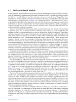
Shih et al. (1995) conducted their experiments in a microchannel using helium as a fluid. The inlet
pressure varied, but the duct exit was atmospheric. Microsensors were fabricated in situ along their
MEMS channel to measure the pressure. Figure 4.4 shows their measured mass flowrateversus the inlet
Flow Physics 4-15
600
400
200
200 > Kn > 17
17 > Kn > 0.6
0.6 > Kn > 0.0
100
0.1 100 1000 10
4
1
80
60
40
20
10
10
8
6
4
(p
2
−p
2
) [Pa
2
]
i
o
m x 10
12
(kg/s)
•
FIGURE 4.3 Variation of mass flowrate as a function of (p
2
i
Ϫ p
2
o
). Original data acquired by S.A. Tison and plotted
by Beskok et al. (1996). (Reprinted with permission from Beskok et al. [1996] “Simulation of Heat and Momentum
Transfer in Complex Micro-Geometries,” J. Thermophys. & Heat Transfer 8, pp. 355–70.)
4
The original data in this figure were acquired by S.A. Tison and plotted by Beskok et al. (1996).
© 2006 by Taylor & Francis Group, LLC
pressure. The data are compared to the no-slip solution and the slip solution using three different values
of the tangential-momentum-accommodation coefficient, 0.8, 0.9, and 1.0. The agreement is reasonable
with the case
σ
v
ϭ 1, indicating perhaps that the channel used by Shih et al., was quite rough on the
molecular scale. In a second experiment [Shih et al., 1996], nitrous oxide was used as the fluid. The square
of the pressure distribution along the channel is plotted for five different inlet pressures in Figure 4.5. The
experimental data (symbols) compare well with the theoretical predictions (solid lines). Again, the non-
linear pressure drop shown indicates that the gas flow is compressible.
Arkilic (1997) provided an elegant analysis of the compressible, rarefied flow in a microchannel. The
results of his theory are compared to the experiments of Pong et al., (1994) in Figure 4.6. The dotted line is
the incompressible flow solution, where the pressure is predicted to drop linearly with streamwise distance.
4-16 MEMS: Introduction and Fundamentals
7
6
5
4
3
2
1
0
0510 15 20 25 30 35
Data
No-slip solution
Slip solution
ν
= 1.0
Slip solution
ν
= 0.9
Slip solution
ν
= 0.8
Inlet pressure (psig)
Mass flow rate × 10
12
(kg/s)
8
FIGURE 4.4 Mass flowrate versus inlet pressure in a microchannel. (Reprinted with permission from Shih et al.
[1995] “Non-Linear Pressure Distribution in Uniform Microchannels,” ASME AMD-MD-Vol. 238, New Yo r k.)
1600
1400
1200
1000
800
600
400
200
0
0 1000 2000
Channel length (µm)
p
2
(psi
2
)
3000 4000
Inlet pressure
8.4 psig
12.1 psig
15.5 psig
19.9 psig
23.0 psig
FIGURE 4.5 Pressure distribution of nitrous oxide in a microduct. Solid lines are theoretical predictions. (Reprinted
with permission from Shih et al. [1996] “Monatomic and Polyatomic Gas Flow through Uniform Microchannels,” in
Applications of Microfabrication to Fluid Mechanics, K. Breuer, P. Bandyopadhyay, and M. Gad-el-Hak, eds., ASME
DSC-Vol. 59, pp. 197–203, New York.)
© 2006 by Taylor & Francis Group, LLC
The dashed line is the compressible flow solution that neglects rarefaction effects (assumes Kn ϭ 0).
Finally, the solid line is the theoretical result that takes into account both compressibility and rarefaction
via slip-flow boundary condition computed at the exit Knudsen number of Kn ϭ 0.06. That theory com-
pares most favorably with the experimental data. In the compressible flow through the constant-area
duct, density decreases and thus velocity increases in the streamwise direction. As a result, the pressure
distribution is nonlinear with negative curvature. A moderate Knudsen number (i.e., moderate slip) actu-
ally diminishes, albeit rather weakly, this curvature. Thus, compressibility and rarefaction effects lead to
opposing trends, as pointed out by Beskok et al. (1996).
4.7 Molecular-Based Models
In the continuum models discussed thus far, the macroscopic fluid properties are the dependent variables
while the independent variables are the three spatial coordinates and time. The molecular models recog-
nize the fluid as a myriad of discrete particles: molecules, atoms, ions, and electrons. The goal here is to
determine the position, velocity, and state of all particles at all times. The molecular approach is either
deterministic or probabilistic (refer to Figure 4.1). Provided that there is a sufficient number of micro-
scopic particles within the smallest significant volume of a flow, the macroscopic properties at any loca-
tion in the flow can then be computed from the discrete-particle information by a suitable averaging or
weighted averaging process. The present section discusses molecular-based models and their relation to
the continuum models previously considered.
The most fundamental of the molecular models is deterministic. The motion of the molecules is gov-
erned by the laws of classical mechanics, although at the expense of greatly complicating the problem, the
laws of quantum mechanics can also be considered in special circumstances. The modern molecular
dynamics computer simulations (MD) have been pioneered by Alder and Wainwright (1957, 1958, 1970)
and reviewed by Ciccotti and Hoover (1986), Allen and Tildesley (1987), Haile (1993), and Koplik and
Banavar (1995). The simulation begins with a set of N molecules in a region of space, each assigned a ran-
dom velocity corresponding to a Boltzmann distribution at the temperature of interest. The interaction
between the particles is prescribed typically in the form of a two-body potential energy and the time evo-
lution of the molecular positions is determined by integrating Newton’s equations of motion. Because
MD is based on the most basic set of equations, it is valid in principle for any flow extent and any range
of parameters. The method is straightforward in principle but there are two hurdles: (1) choosing a
Flow Physics 4-17
2.8
2.4
0.8
0.2
Nondimensional position (x)
Nondimensional pressure
0.4 0.6 0.80 1
1.6
1.2
2
Pong et al. (1994)
Outlet Knudsen number = 0.0
Outlet Knudsen number = 0.06
Incompressible flow solution
FIGURE 4.6 Pressure distribution in a long microchannel. The symbols are experimental data while the lines are
different theoretical predictions. (Reprinted with permission from Arkilic [1997] Measurement of the Mass Flow and
Tangential Momentum Accommodation Coefficient in Silicon Micromachined Channels, Ph.D. thesis, Massachusetts
Institute of Technology.)
© 2006 by Taylor & Francis Group, LLC
proper and convenient potential for particular fluid and solid combinations, and (2) the colossal
computer resources required to simulate a reasonable flowfield extent.
For purists, the former difficulty is a sticky one. There is no totally rational methodologybywhich a
convenient potential can be chosen. Part of the art of MD is to pick an appropriate potential and validate
the simulation results with experiments or other analytical/computational results. Acommonly used
potential between two molecules is the generalized Lennart-Jones 6–12 potential, to be used in the
following section and further discussed in the section following that.
The second difficulty, and by far the most serious limitation of molecular dynamics simulations, is the
number of molecules N that can realistically be modeled on a digital computer. Since the computation of
an element of trajectory for any particular molecule requires consideration of all other molecules as
potential collision partners, the amount of computation required by the MD method is proportional to N
2
.
Some savings in computer time can be achieved by cutting off the weak tail of the potential (see Figure 4.11)
at, say, r
c
ϭ 2.5
σ
, and shifting the potential by a linear term in r so that the force goes smoothly to zero
at the cutoff. As a result, only nearby molecules are treated as potential collision partners, and the
computation time for N molecules no longer scales with N
2
.
The state of the art of molecular dynamics simulations in the early 2000s is such that with a few hours
of CPU time general purpose supercomputers can handle around 100,000 molecules. At enormous
expense, the fastest parallel machine available can simulate around 10 million particles. Because of the
extreme diminution of molecular scales, the above translates into regions of liquid flow of about 0.06µm
(600 angstroms) in linear size, over time intervals of around 0.001 µsec, enough for continuum behavior
to set in for simple molecules. To simulate 1 sec of real time for complex molecular interactions (e.g.,
vibration modes, reorientation of polymer molecules, collision of colloidal particles, etc.) requires
unrealistic CPU time measured in hundreds of years.
MD simulations are highly inefficient for dilute gases where the molecular interactions are infrequent.
The simulations are more suited for dense gases and liquids. Clearly, molecular dynamics simulations are
reserved for situations where the continuum approach or the statistical methods are inadequate to com-
pute from first principles important flow quantities. Slip boundary conditions for liquid flows in
extremely small devices are such a case, as will be discussed in the following section.
An alternative to the deterministic molecular dynamics is the statistical approach where the goal is to
compute the probability of finding a molecule at a particular position and state. If the appropriate con-
servation equation can be solved for the probability distribution, important statistical properties, such as
the mean number, momentum, or energy of the molecules within an element of volume, can be com-
puted from a simple weighted averaging. In a practical problem, it is such average quantities that concern
us rather than the detail for every single molecule. Clearly, however, the accuracy of computing average
quantities via the statistical approach improves as the number of molecules in the sampled volume
increases. The kinetic theory of dilute gases is well advanced, but that of dense gases and liquids is much
less so due to the extreme complexity of having to include multiple collisions and intermolecular forces
in the theoretical formulation. The statistical approach is well covered in books such as those by Kennard
(1938), Hirschfelder et al. (1954), Schaaf and Chambré (1961), Vincenti and Kruger (1965), Kogan
(1969), Chapman and Cowling (1970), Cercignani (1988, 2000) and Bird (1994), and review articles such
as those by Kogan (1973), Muntz (1989), and Oran et al. (1998).
In the statistical approach, the fraction of molecules in a given location and state is the sole dependent
variable. The independent variables for monatomic molecules are time, the three spatial coordinates, and
the three components of molecular velocity. Those describe a six-dimensional phase space.
5
For diatomic
or polyatomic molecules, the dimension of phase space is increased by the number of internal degrees of
freedom. Orientation adds an extra dimension for molecules that are not spherically symmetric. Finally,
for mixtures of gases, separate probability distribution functions are required for each species. Clearly, the
4-18 MEMS: Introduction and Fundamentals
5
The evolution equation of the probability distribution is considered, hence time is the seventh independent variable.
© 2006 by Taylor & Francis Group, LLC
complexity of the approach increases dramatically as the dimension of phase space increases. The sim-
plest problems are, for example, those for steady, one-dimensional flow of a simple monatomic gas.
To simplify the problem we restrict the discussion here to monatomic gases having no internal degrees
of freedom. Furthermore, the fluid is restricted to dilute gases and molecular chaos is assumed. The for-
mer restriction requires the average distance between molecules
δ
to be an order of magnitude larger than
their diameter
σ
. That will almost guarantee that all collisions between molecules are binary collisions,
avoiding the complexity of modeling multiple encounters.
6
The molecular chaos restriction improves the
accuracy of computing the macroscopic quantities from the microscopic information. In essence, the vol-
ume over which averages are computed has to have enough molecules to reduce statistical errors. It can
be shown that computing macroscopic flow properties by averaging over a number of molecules will
result in statistical fluctuations with a standard deviation of approximately 0.1% if one million molecules
are used and around 3% if one thousand molecules are used. The molecular chaos limit requires the
length-scale L for the averaging process to be at least 100 times the average distance between molecules
(i.e., typical averaging over at least one million molecules).
Figure 4.7, adapted from Bird (1994), shows the limits of validity of the dilute gas approximation
(
δ
/
σ
Ͼ 7), the continuum approach (Kn Ͻ 0.1, as discussed previously), and the neglect of statistical
fluctuations (L/
δ
Ͼ 100). Using a molecular diameter of
σ
ϭ 4 ϫ10
–10
m as an example, the three limits
are conveniently expressed as functions of the normalized gas density
ρ
/
ρ
o
or number density n/n
o
, where
the reference densities
ρ
o
and n
o
are computed at standard conditions. All three limits are straight lines in
Flow Physics 4-19
Microscopic approach nec
essary
Insignificant fluctuations
(
L/
␦
> 100)
Significant statistical fluctuations
Navier–Stokes e
quations valid
(
kn
< 0.1)
Dilute gas
(
␦/
> 7)
Dense gas
Characteristic dimension L (meter)
10
2
1
10
−2
10
−
4
10
−6
10
−8
10
−8
10
−6
10
−4
10
−2
1 10
2
10
10
10
8
10
6
10
4
10
2
10,000 1,000 100 10 3
L
␦/
Density ratio
n
/
n
o
or /
o
FIGURE 4.7 Effective limits of different flow models. (Reprinted with permission from Bird [1994] Molecular Gas
Dynamics and the Direct Simulation of Gas Flows, Clarendon Press, Oxford.)
6
Dissociation and ionization phenomena involve triple collisions and therefore require separate treatment.
© 2006 by Taylor & Francis Group, LLC
the log–log plot of L versus
ρ
/
ρ
o
, as depicted in Figure 4.7.Note the shaded triangular wedge inside which
both the Boltzmann and Navier–Stokes equations are valid. Additionally, the lines describing the three
limits very nearly intersect at a single point. As a consequence, the continuum breakdown limit always lies
between the dilute gas limit and the limit for molecular chaos. As density or characteristic dimension is
reduced in a dilute gas, the Navier–Stokes model breaks down before the level of statistical fluctuations
becomes significant. In a dense gas, on the other hand, significant fluctuations may be present even when
the Navier–Stokes model is still valid.
The starting point in statistical mechanics is the Liouville equation, which expresses the conservation
of the N-particle distribution function in 6N-dimensional phase space,
7
where N is the number of
particles under consideration. Considering only external forces that do not depend on the velocity of the
molecules,
8
the Liouville equation for a system of N mass points reads
ϩ
Α
N
kϭ1
ξ
→
k и ϩ
Α
N
kϭ1
F
→
k
и = 0 (4.51)
where Ᏺ is the probability of finding a molecule at a particular point in phase space, t is time,
ξ
→
k
is the
three-dimensional velocity vector for the kth molecule, x
→
k
is the three-dimensional position vector for the
kth molecule, and F
→
is the external force vector. Note that the dot product in Equation (4.51) is carried
out over each of the three components of the vectors
ξ
→
, x
→
and F
→
and that the summation is overall mol-
ecules. Obviously such an equation is not tractable for a realistic number of particles.
A hierarchy of reduced distribution functions may be obtained by repeated integration of the Liouville
equation above. The final equation in the hierarchy is for the single particle distribution, which also involves
the two-particle distribution function. Assuming molecular chaos, that final equation becomes a closed
one (i.e., one equation in one unknown) and is known as the Boltzmann equation, the fundamental relation
of the kinetic theory of gases. That final equation in the hierarchy is the only one that offers any hope of
obtaining analytical solutions.
A simpler direct derivation of the Boltzmann equation is provided by Bird (1994). For monatomic gas
molecules in binary collisions, the integro-differential Boltzmann equation reads
ϩ
ξ
j
ϩ F
j
ϭ J( f, f *), j ϭ 1, 2, 3 (4.52)
where nf is the product of the number density and the normalized velocity distribution function
(dn/n ϭ fd
ξ
→
), x
j
, and
ξ
j
are respectively the coordinates and speeds of a molecule,
9
F
j
is a known external
force, and J( f, f *)is the nonlinear collision integral that describes the net effect of populating and depop-
ulating collisions on the distribution function. The collision integral is the source of difficulty in obtain-
ing analytical solutions to the Boltzmann equation and is given by
J( f, f *) ϭ
͵
ϱ
Ϫϱ
͵
4
π
0
n
2
( f *f *
1
Ϫ f f
1
)
ξ
→
r
σ
dΩ(d
ξ
→
)
1
(4.53)
where the superscript * indicates postcollision values, f and f
1
represent two different molecules,
ξ
→
r
is the
relative speed between two molecules,
σ
is the molecular cross-section, Ω is the solid angle, and
d
ξ
→
ϭ d
ξ
1
d
ξ
2
d
ξ
3
.
Once a solution for f is obtained, macroscopic quantities, such as density, velocity, and temperature,
can be computed from the appropriate weighted integral of the distribution function. For example,
ρ
ϭ mn ϭ m͵(n f )d
ξ
→
(4.54)
u
i
ϭ ͵
ξ
i
fd
ξ
→
(4.55)
∂(nf)
ᎏ
∂
ξ
j
∂(nf)
ᎏ
∂x
j
∂(nf)
ᎏ
∂t
∂Ᏺ
ᎏ
∂
ξ
→
k
∂Ᏺ
ᎏ
∂
x
→
k
∂Ᏺ
ᎏ
∂t
4-20 MEMS: Introduction and Fundamentals
7
Three positions and three velocities for each molecule of a monatomic gas with no internal degrees of freedom.
8
This excludes Lorentz forces, for example.
9
Constituting together with time the seven independent variables of the single-dependent-variable equation.
© 2006 by Taylor & Francis Group, LLC
kT ϭ ∫ m
ξ
i
ξ
i
fdξ
→
(4.56)
If the Boltzmann equation is nondimensionalized with a characteristic length L and characteristic
speed [2(k/m)T]
1/2
,wherek is the Boltzmann constant, m is the molecular mass, and T is temperature,
the inverse Knudsen number appears explicitly in the right-hand side of the equation as follows:
ϩ
ξ
j
ϩ
F
j
ϭ J
(
f ,
f
*
),
j
ϭ 1, 2, 3
(4.57)
where the topping symbol
represents a dimensionless variable, and
f is nondimensionalized using a
reference number density n
o
.
The five conservation equations for the transport of mass, momentum, and energy can be derived by
multiplying the Boltzmann equation above by the molecular mass, momentum, and energy respectively,
then integrating overall possible molecular velocities. Subject to the restrictions of dilute gas and molec-
ular chaos stated earlier, the Boltzmann equation is valid for all ranges of Knudsen number from 0 to ∞.
Analytical solutions to this equation for arbitrary geometries are difficult mostly because of the nonlin-
earity of the collision integral. Simple models of this integral have been proposed to facilitate analytical
solutions [see, for example, Bhatnagar et al. (1954)].
There are two important asymptotes to Equation (4.57). First, as Kn →∞, molecular collisions become
unimportant.This is the free-molecule flow regime depicted in Figure 4.2 for Kn Ͼ 10, where the only impor-
tant collision is that between a gas molecule and the solid surface of an obstacle or a conduit. Analytical solu-
tions are then possible for simple geometries, and numerical simulations for complicated geometries are
straightforward once the surface-reflection characteristics are accurately modeled. Second, as Kn → 0, colli-
sions become important and the flow approaches the continuum regime of conventional fluid dynamics. The
Second Law specifies a tendency for thermodynamic systems to revert to equilibrium state, smoothing any
discontinuities in macroscopic flow quantities. The number of molecular collisions in the limit Kn → 0 is so
large that the flow approaches the equilibrium state in a time that is short compared to the macroscopic time-
scale. For example, for air at standard conditions (T ϭ 288 K; p ϭ 1 atm), each molecule experiences on
average 10 collisions per nanosecond and travels 1 micron in the same time. Such a molecule has already for-
gotten its previous state after 1nsec. In a particular flowfield, if the macroscopic quantities vary little over a
distance of 1 µm or over a time interval of 1 nsec, the flow of STP air is near equilibrium.
At Kn ϭ 0, the velocity distribution function is everywhere of the local equilibrium or Maxwellian form
f
(0)
ϭ
π
Ϫ3/2
exp[Ϫ(
ξ
Ϫ
u)
2
] (4.58)
where
ξ
and u
are the dimensionless speeds respectively of a molecule and of the flow. In this Knudsen
number limit, the velocity distribution of each element of the fluid instantaneously adjusts to the equi-
librium thermodynamic state appropriate to the local macroscopic properties as this molecule moves
through the flow field. From the continuum viewpoint, the flow is isentropic, and heat conduction and
viscous diffusion and dissipation vanish from the continuum conservation relations.
The Chapman–Enskog theory attempts to solve the Boltzmann equation by considering a small per-
turbation of f
from the equilibrium Maxwellian form. For small Knudsen numbers, the distribution
function can be expanded in terms of Kn in the form of a power series
f ϭ
f
(0)
ϩ Kn
f
(1)
ϩ Kn
2
f
(2)
ϩ
…
(4.59)
By substituting the above series in the Boltzmann Equation (4.57) and equating terms of equal order, we
arrive at the following recurrent set of integral equations:
J
(
f
(0)
,
f
(0)
) ϭ 0,
J(
f
(0)
,
f
(1)
) ϭ
ϩ
ξ
j
ϩ
F
j
,
…
(4.60)
∂
f
(0)
ᎏ
∂
ξ
j
∂
f
(0)
ᎏ
∂
x
j
∂
f
ᎏ
∂
t
n
ᎏ
n
o
1
ᎏ
Kn
∂
f
ᎏ
∂
ξ
j
∂
f
ᎏ
∂x
j
∂
f
ᎏ
∂
t
1
ᎏ
2
3
ᎏ
2
Flow Physics 4-21
© 2006 by Taylor & Francis Group, LLC
The first integral is nonlinear, and its solution is the local Maxwellian distribution, Equation (4.58). Each
of the distribution functions
f
(1)
,
f
(2)
, etc., satisfies an inhomogeneous linear equation whose solution
leads to the transport terms needed to close the continuum equations appropriate to the particular level
of approximation. The continuum stress tensor and heat flux vector can be written in terms of the dis-
tribution function, which in turn can be specified in terms of the macroscopic velocity and temperature
and their derivatives [Kogan, 1973]. The zeroth-order equation yields the Euler equations, the first-order
equation results in the linear transport terms of the Navier–Stokes equations, the second-order equation
gives the nonlinear transport terms of the Burnett equations, and so on. Keep in mind, however, that the
Boltzmann equation as developed in this section is for a monatomic gas. This excludes the all-important
air, which is composed largely of diatomic nitrogen and oxygen.
As discussed earlier, the Navier–Stokes equations can and should be used up to a Knudsen number of 0.1.
Beyond that, the transition flow regime commences (0.1 Ͻ Kn Ͻ 10). In this flow regime, the molecular
mean free path for a gas becomes significant relative to a characteristic distance for important flow-
property changes to take place. The Burnett equations can be used to obtain analytical/numerical solu-
tions for at least a portion of the transition regime for a monatomic gas, although their complexity has
limited the results for realistic geometries (Agarwal et al., 1999, 2001; Lockerby and Reese, 2003). There
is also a certain degree of uncertainty about the proper boundary conditions to use with the continuum
Burnett equations, and experimental validation of the results has been very scarce. Additionally, as the gas
flow departs farther from equilibrium, the bulk viscosity (ϭ
λ
ϩ
ᎏ
2
3
ᎏ
µ
, where
λ
is the second coefficient of
viscosity) is no longer zero, and Stokes’ hypothesis no longer holds (see Gad-el-Hak, 1995, for an
interesting summary of the issue of bulk viscosity).
In the transition regime, the molecularly-based Boltzmann equation cannot easily be solved either, unless
the nonlinear collision integral is simplified. So, clearly, the transition regime is in dire need of alterna-
tive solutions. MD simulations as mentioned earlier are not suited for dilute gases. The best approach for
the transition regime right now is the direct simulation Monte Carlo (DSMC) method developed by Bird
(1963, 1965, 1976, 1978, 1994) and briefly described below. Some recent reviews of DSMC include those
by Muntz (1989), Cheng (1993), Cheng and Emmanuel (1995), and Oran et al. (1998). The mechanics as
well as the history of the DSMC approach and its ancestors are well described in Bird (1994).
Unlike molecular dynamics simulations, DSMC is a statistical computational approach to solving rar-
efied gas problems. Both approaches treat a gas as discrete particles. Subject to the dilute gas and molec-
ular chaos assumptions, the direct simulation Monte Carlo method is valid for all ranges of Knudsen
number, although it becomes quite expensive for Kn Ͻ 0.1. Fortunately, this is the continuum regime
where the Navier–Stokes equations can be used analytically or computationally. DSMC is therefore ideal
for the transition regime (0.1 Ͻ Kn Ͻ 10), where the Boltzmann equation is difficult to solve. The Monte
Carlo method is, like its namesake, a random-number strategy based directly on the physics of the indi-
vidual molecular interactions. The idea is to track a large number of randomly selected, statistically rep-
resentative particles, and to use their motions and interactions to modify their positions and states. The
primary approximation of the direct simulation Monte Carlo method is to uncouple the molecular
motions and the intermolecular collisions over small time intervals. A significant advantage of this
approximation is that the amount of computation required is proportional to N, in contrast to N
2
for
molecular dynamics simulations. In essence, particle motions are modeled deterministically, while colli-
sions are treated probabilistically, each simulated molecule representing a large number of actual mole-
cules. Typical computer runs of DSMC in the 1990s involved tens of millions of intermolecular collisions
and fluid–solid interactions.
The DSMC computation is started from some initial condition and followed in small time steps that
can be related to physical time. Colliding pairs of molecules in a small geometric cell in physical space are
randomly selected after each computational time step. Complex physics such as radiation, chemical reac-
tions, and species concentrations can be included in the simulations without the necessity of nonequilib-
rium thermodynamic assumptions that commonly afflict nonequilibrium continuum-flow calculations.
DSMC is more computationally intensive than classical continuum simulations, and should therefore be
used only when the continuum approach is not feasible.
4-22 MEMS: Introduction and Fundamentals
© 2006 by Taylor & Francis Group, LLC
The DSMC technique is explicit and time marching and therefore always produces unsteady flow sim-
ulations. For macroscopically steady flows, Monte Carlo simulation proceeds until a steady flow is estab-
lished within a desired accuracy at sufficiently large time. The macroscopic flow quantities are then the
time average of all values calculated after reaching the steady state. For macroscopically unsteady flows,
ensemble averaging of many independent Monte Carlo simulations is carried out to obtain the final
results within a prescribed statistical accuracy.
4.8 Liquid Flows
From the continuum point of view, liquids and gases are both fluids obeying the same equations of
motion. For incompressible flows, for example, the Reynolds number is the primary dimensionless param-
eter that determines the nature of the flow field. True, water, for example, has density and viscosity that are
respectively three orders and two orders of magnitude higher than those for air, but if the Reynolds num-
ber and geometry are matched, liquid and gas flows should be identical.
10
For MEMS applications, how-
ever, we anticipate the possibility of nonequilibrium flow conditions and the consequent invalidity of the
Navier–Stokes equations and the no-slip boundary conditions. Such circumstances can best be researched
using the molecular approach. We discussed this for gases earlier and will give the corresponding argu-
ments for liquids in the present section. The literature on non-Newtonian fluids in general and polymers
in particular is vast (for example, the bibliographic survey by Nadolink and Haigh, 1995, cites over 4,900
references on polymer drag reduction alone) and provides a rich source of information on the molecu-
lar approach for liquid flows.
Solids, liquids, and gases are distinguished merely by the degree of proximity and the intensity of motions
of their constituent molecules. In solids, the molecules are packed closely and confined, each hemmed in
by its neighbors [Chapman and Cowling, 1970]. Only rarely would one solid molecule slip from its neigh-
bors to join a new set. As the solid is heated, molecular motion becomes more violent, and a slight ther-
mal expansion takes place. At a certain temperature that depends on ambient pressure, sufficiently intense
motion of the molecules enables them to pass freely from one set of neighbors to another. The molecules
are no longer confined but are nevertheless still closely packed, and the substance is now considered a liquid.
Further heating of the matter eventually releases the molecules altogether, allowing them to break the bonds
of their mutual attractions. Unlike solids and liquids, the resulting gas expands to fill any available volume.
Unlike solids, neither liquids nor gases can resist finite shear force without continuous deformation; that
is, the definition of a fluid medium. In contrast to the reversible, elastic, static deformation of a solid, the con-
tinuous deformation of a fluid resulting from the application of a shear stress results in an irreversible
work that eventually becomes random thermal motion of the molecules — that is, viscous dissipation.
There are around 25 million molecules of STP air in a 1 µm cube. The same cube would contain around
34 billion molecules of water. So liquid flows are a continuum even in extremely small devices through
which gas flows would not be a continuum. The average distance between molecules in the gas example is
one order of magnitude higher than the diameter of its molecules, while that for the liquid phase
approaches the molecular diameter. As a result, liquids are almost incompressible. Their isothermal com-
pressibility coefficient
α
and bulk expansion coefficient
β
are much smaller than those for gases. For water,
for example, a hundredfold increase in pressure leads to a less than 0.5% decrease in volume. Sound speeds
through liquids are also higher than through gases, and as a result most liquid flows are incompressible.
11
The exception is the propagation of ultra-high-frequency sound waves and cavitation phenomena.
The mechanism by which liquids transport mass, momentum, and energy must be very different from that
for gases. In dilute gases, intermolecular forces play no role, and the molecules spend most of their time
in free flight between brief collisions that abruptly change their direction and speed. The random molecular
motions are responsible for gaseous transport processes. In liquids, on the other hand, the molecules are
Flow Physics 4-23
10
Barring phenomena unique to liquids such as cavitation, free surface flows, etc.
11
Note that we distinguish between a fluid’s and a flow’s being compressible/incompressible. For example, the
flow of the highly compressible air can be either compressible or incompressible.
© 2006 by Taylor & Francis Group, LLC
closely packed though not fixed in one position. In essence, the liquid molecules are always in a collision state.
Applying a shear force must create a velocity gradient so that the molecules move relative to one another,
ad infinitum as long as the stress is applied. For liquids, momentum transport due to the random molec-
ular motion is negligible compared to that due to the intermolecular forces. The straining between liquid
molecules causes some to separate from their original neighbors, bringing them into the force field of new
molecules. Across the plane of the shear stress, the sum of all intermolecular forces must, on average, balance
the imposed shear. Liquids at rest transmit only normal force, but when a velocity gradient occurs, the net
intermolecular force has a tangential component.
The incompressible Navier–Stokes equations describe liquid flows under most circumstances. Liquids,
however, do not have a well-advanced molecular-based theory like that for dilute gases. The concept of
mean free path is not very useful for liquids, and the conditions under which a liquid flow fails to be in
quasi-equilibrium state are not well defined. There is no Knudsen number to guide us through the maze
of liquid flows. We do not know from first principles the conditions under which the no-slip boundary
condition becomes inaccurate or the point at which the stress–rate of strain relation or the heat flux–
temperature gradient relation fails to be linear. Certain empirical observations indicate that those simple
relations that we take for granted occasionally fail to accurately model liquid flows. For example, it has
been shown in rheological studies (Loose and Hess, 1989) that non-Newtonian behavior commences
when the strain rate approximately exceeds twice the molecular frequency-scale
γ
.
ϭ у 2 ᐀
Ϫ1
(4.61)
where the molecular time-scale ᐀ is given by
᐀ ϭ
΄
΅
(4.62)
where m is the molecular mass, and
σ
and
ε
are respectively the characteristic length- and energy-scale for
the molecules. For ordinary liquids such as water, this time-scale is extremely small and the threshold shear
rate for the onset of non-Newtonian behavior is therefore extraordinarily high. For high-molecular-weight
polymers, on the other hand, m and
σ
are both many orders of magnitude higher than their respective
values for water, and the linear stress–strain relation breaks down at realistic values of the shear rate.
The moving contact line when a liquid spreads on a solid substrate is an example where slip-flow must
be allowed to avoid singular or unrealistic behavior in the Navier–Stokes solutions [Dussan and Davis,
1974; Dussan, 1976, 1979; Thompson and Robbins, 1989]. Other examples where slip-flow must be
admitted include corner flows [Moffatt, 1964; Koplik and Banavar, 1995] and extrusion of polymer melts
from capillary tubes [Pearson and Petrie, 1968; Richardson, 1973; Den, 1990].
Existing experimental results of liquid flow in microdevices are contradictory. This is not surprising
given the difficulty of such experiments and the lack of a guiding rational theory. Pfahler et al. (1990,
1991), Pfahler (1992), and Bau (1994) summarize the relevant literature. For small-length-scale flows,
a phenomenological approach for analyzing the data is to define an apparent viscosity
µ
a
calculated so
that if it were used in the traditional no-slip Navier–Stokes equations instead of the fluid viscosity
µ
, the
results would be in agreement with experimental observations. Israelachvili (1986) and Gee et al. (1990)
found that
µ
a
ϭ
µ
for thin-film flows as long as the film thickness exceeds 10 molecular layers (ഠ5 nm).
For thinner films,
µ
a
depends on the number of molecular layers and can be as much as 10
5
times larger
than
µ
. Chan and Horn’s (1985) results are somewhat different: the apparent viscosity deviates from the
fluid viscosity for films thinner than 50 nm.
In polar-liquid flows through capillaries, Migun and Prokhorenko (1987) report that
µ
a
increases for
tubes smaller than 1 µm in diameter. In contrast, Debye and Cleland (1959) report
µ
a
smaller than
µ
for
paraffin flow in porous glass with average pore size several times larger than the molecular length-scale.
Experimenting with microchannels ranging in depths from 0.5 µm to 50 µm, Pfahler, et al. (1991) found
that
µ
a
is consistently smaller than
µ
for both liquid (isopropyl alcohol, silicone oil) and gas (nitrogen,
helium) flows in microchannels. For liquids, the apparent viscosity decreases with decreasing channel
1
ᎏ
2
m
σ
2
ᎏ
ε
∂u
ᎏ
∂y
4-24 MEMS: Introduction and Fundamentals
© 2006 by Taylor & Francis Group, LLC
depth. Other researchers using small capillaries report that
µ
a
is about the same as
µ
[Anderson and
Quinn, 1972; Tukermann and Pease, 1981, 1982; Tuckermann, 1984; Guvenc, 1985; Nakagawa et al., 1990].
Very recently, Sharp (2001) and Sharp et al. (2001) asserted that, despite the significant inconsistencies
in the literature regarding liquid flows in microchannels, such flows are well predicted by macroscale con-
tinuum theory. A case can be made to the contrary, however, as will be seen at the end of this section, and
the final verdict on this controversy is yet to come.
The above contradictory results point to the need for replacing phenomenological models with first-
principles models. The lack of molecular-based theory of liquids — despite extensive research by the rhe-
ology and polymer communities — leaves molecular dynamics simulations as the nearest alternative to a
first-principles model. MD simulations offer a unique approach to checking the validity of the traditional
continuum assumptions. However, as was pointed out earlier, such simulations are limited to exceedingly
minute flow extent.
Thompson and Troian (1997) provide molecular dynamics simulations to quantify the slip-flow bound-
ary condition dependence on shear rate. Recall the linear Navier boundary condition introduced earlier
∆u|
w
ϭ u
fluid
Ϫ u
wall
ϭ L
s
Έ
w
(4.63)
where L
s
is the constant slip length, and
Έ
w
is the strain rate computed at the wall. The goal of Thompson and Troian’s simulations was to determine
the degree of slip at a solid–liquid interface as the interfacial parameters and the shear rate change. In
their simulations, a simple liquid underwent planar shear in a Couette cell as shown in Figure 4.8. The
∂u
ᎏ
∂y
∂u
ᎏ
∂y
Flow Physics 4-25
1
x
U
h
y
Solid
Solid
Fluid
0
0
y/h
1
∈
wf
wf
n
w
0.5
0.5
0.6
0.6
0.2
1
4
4
1.0
0.75
0.75
u(y)/U
FIGURE 4.8 Velocity profiles in a Couette flow geometry at different interfacial parameters. All three profiles are for
U ϭ
σ
᐀
Ϫ1
, and h ϭ 24.57
σ
. The dashed line is the no-slip Couette-flow solution. (Reprinted with permission from
Thompson and Troian [1997] “A General Boundary Condition for Liquid Flow at Solid Surfaces,” Nature 389,
pp. 360–62.)
© 2006 by Taylor & Francis Group, LLC
typical cell measured 12.51 ϫ 7.22 ϫ h, in units of molecular length-scale
σ
,where the channel depth h
varied in the range of 16.71
σ
–24.57
σ
, and the corresponding number of molecules simulated ranged from
1,152 to 1,728. The liquid is treated as an isothermal ensemble of spherical molecules. A shifted
L
ennart-Jones 6–12 potential is used to model intermolecular interactions, with energy- and length-scales
ε
and
σ
, and cut-off distance r
c
ϭ 2.2
σ
:
V(r) ϭ 4
ε
΄
Ϫ12
Ϫ
Ϫ6
Ϫ
Ϫ12
ϩ
Ϫ6
΅
(4.64)
The truncated potential is set to zero for r Ͼ r
c
.
The fluid–solid interaction is also modeled with a truncated Lennart-Jones potential, with energy- and
length-scales
ε
wf
and
σ
wf
, and cut-off distance r
c
.The equilibrium state of the fluid is a well-defined liq-
uid phase characterized by number density n ϭ 0.81
σ
Ϫ3
and temperature T ϭ 1.1
ε
/k,wherek is the
Boltzmann constant.
The steady state velocity profiles resulting from Thompson and Tr oian’s (1997) MD simulations are
depicted in Figure 4.8 for different values of the interfacial parameters
ε
wf
,
σ
wf
, and n
w
.Those parameters,
shown in units of the corresponding fluid parameters
ε
,
σ
, and n,characterize respectively the strength of the
liquid–solid coupling, the thermal roughness of the interface, and the commensurability of wall and liquid
densities. The macroscopic velocity profiles recover the expected flow behavior from continuum hydrody-
namics with boundary conditions involving varying degrees of slip. Note that when slip exists, the shear rate
γ
.
no longer equals U/h.The degree of slip increases (i.e., the amount of momentum transfer at the wall–fluid
interface decreases) as the relative wall density n
w
increases or the strength of the wall–fluid coupling
σ
wf
decreases — in other words, when the relative surface energy corrugation of the wall decreases. Conversely,
the corrugation is maximized when the wall and fluid densities are commensurate and the strength of the
wall–fluid coupling is large. In this case, the liquid feels the corrugations in the surface energy of the solid
owing to the atomic close-packing. Consequently, there is efficient momentum transfer, and the no-slip con-
dition applies, or in extreme cases, a“stick” boundary condition takes hold.
Var iations of the slip length L
s
and viscosity
µ
as functions of shear rate
γ
.
are shown in Figure 4.9 for
five different sets of interfacial parameters. For Couette flow, the slip length is computed from its definition,
∆u|
w
/
γ
.
ϭ (U/
γ
.
Ϫ h)/2. The slip length, viscosity, and shear rate are normalized in the figure using the
respective molecular scales for length
σ
,viscosity
ε
᐀
σ
Ϫ3
, and inverse time ᐀
Ϫ1
.The viscosity of the fluid
is constant over the entire range of shear rates (Figure 4.9b) indicating Newtonian behavior. As indicated
earlier, non-Newtonian behavior is expected for
γ
.
у 2᐀
Ϫ1
,well above the shear rates used in Thompson
and Tr oian’s simulations.
At low shear rates, the slip length behavior is consistent with the Navier model (i.e., is independent of
the shear rate). Its limiting value L
o
s
ranges from 0 to ϳ17
σ
for the range of interfacial parameters chosen
(Figure 4.9a). In general, the amount of slip increases with decreasing surface energy corrugation. Most
interestingly, at high shear rates the Navier condition breaks down as the slip length increases rapidly with
γ
.
c
.The critical shear-rate value for the slip length to diverge,
γ
.
c
,decreases as the surface energy corrugation
decreases. Surprisingly, the boundary condition is nonlinear even though the liquid is still Newtonian. In
dilute gases, the linear slip condition and the Navier–Stokes equations, with their linear stress–strain rela-
tion, are both valid to the same order of approximation in Knudsen number. In other words, deviation
from linearity is expected to take place at the same value of Kn ϭ 0.1. In liquids, in contrast, the slip
length appears to become nonlinear and to diverge at a critical value of shear rate well below the shear
rate at which the linear stress–strain relation fails. Moreover, the boundary condition deviation from lin-
earity is not gradual but is rather catastrophic. The critical value of shear rate
γ
.
c
signals the point at which
the solid can no longer impart momentum to the liquid. This means that the same liquid molecules
sheared against different substrates will experience varying amounts of slip and vice versa.
Based on the above results, Thompson and Troian (1997) suggest a universal boundary condition at a
solid–liquid interface. Scaling the slip length L
s
by its asymptotic limiting value L
o
s
and the shear rate
γ
.
by
its critical value
γ
.
c
collapses the data in the single curve shown in Figure 4.10. The data points are well
described by the relation
r
c
ᎏ
σ
r
c
ᎏ
σ
r
ᎏ
σ
r
ᎏ
σ
4-26 MEMS: Introduction and Fundamentals
© 2006 by Taylor & Francis Group, LLC
L
s
ϭ L
o
s
΄
1 Ϫ
΅
Ϫ
(4.65)
The nonlinear behavior close to a critical shear rate suggests that the boundary condition can signifi-
cantly affect flow behavior at macroscopic distances from the wall. Experiments with polymers confirm
this observation [Atwood and Schwalter, 1989]. The rapid change in the slip length suggests that for flows
in the vicinity of
γ
.
c
, small changes in surface properties can lead to large fluctuations in the apparent
boundary condition. Thompson and Troian (1997) conclude that the Navier slip condition is but the
low-shear-rate limit of a more generalized universal relationship that is nonlinear and divergent. Their
relation provides a mechanism for relieving the stress singularity in spreading contact lines and corner
flows, as it naturally allows for varying degrees of slip on approach to regions of higher rate of strain.
To place the above results in physical terms, consider water
12
at a temperature of T ϭ 288 K. The
energy-scale in the Lennart-Jones potential is then
ε
ϭ 3.62 ϫ 10
–21
J. For water, m ϭ 2.99 ϫ 10
–26
kg,
σ
ϭ 2.89 ϫ 10
–10
m, and at standard temperature n ϭ 3.35 ϫ 10
28
molecules/m
3
. The molecular time-scale
can thus be computed,
᐀ ϭ [m
σ
2
/
ε
] ϭ 8.31 ϫ 10
Ϫ13
s
1
ᎏ
2
1
ᎏ
2
γ
.
ᎏ
γ
.
c
Flow Physics 4-27
40
30
20
10
(b)
(a)
0
3
2
1
0
0.001 0.01 0.1 1.0
0.6
0.1
0.6
0.4
0.2
1
1
4
4
4
1.0
1.0
0.75
0.75
0.75
∈
wf
wf
n
w
/
∈
t
s
−3 L
s
/
s
␥
t
FIGURE 4.9 Variation of slip length and viscosity as functions of shear rate. (Reprinted with permission from
Thompson and Troian [1997] “A General Boundary Condition for Liquid Flow at Solid Surfaces,” Nature 389,
pp. 360–62.)
12
Water molecules are complex, forming directional, short-range covalent bonds and thus requiring a more com-
plex potential than the Lennart-Jones to describe the intermolecular interactions. For the purpose of the qualitative
example described here, however, we use the computational results of Thompson and Troian (1997), who employed
the L–J potential.
© 2006 by Taylor & Francis Group, LLC
For the third case depicted in Figure 4.10 (the open squares),
γ
.
c
᐀ ϭ 0.1, and the critical shear rate at
which the slip condition diverges is thus
γ
.
c
ϭ 1.2 ϫ 10
11
s
Ϫ1
.Such an enormous rate of strain
13
may be
found in extremely small devices having extremely high speeds. On the other hand, the conditions to
achieve a measurable slip of 17
σ
(the solid circles in Figure 4.9) are not difficult to encounter in microde-
vices: density of solid that is four times that of liquid, and energy-scale for wall-fluid interaction that is
one-fifth of energy-scale for liquid.
The limiting value of slip length is independent of the shear rate and can be computed for water as
L
o
s
ϭ 17
σ
ϭ 4.91 ϫ10
Ϫ9
m. Consider a water microbearing having a shaft diameter of 100 µm, arotation
rate of 20,000 rpm, and a minimum gap of h ϭ 1 µm. In this case, U ϭ 0.1 m/sec, and the no-slip shear
rate is U/h ϭ 10
5
s
–1
.When slip occurs at the limiting value just computed, the shear rate and the wall
slip-velocity are computed as follows
γ
.
ϭ ϭ 9.90 ϫ10
4
s
Ϫ1
(4.66)
∆u|
w
ϭ
γ
.
L
s
ϭ 4.87 ϫ10
Ϫ4
m/s (4.67)
As a result of the Navier slip, the shear rate is reduced by 1% from its no-slip value, and the slip velocity
at the wall is about 0.5% of U, small but not insignificant.
4.9 Surface Phenomena
The surface-to-volume ratio for a machine with a characteristic length of 1 m is 1 m
Ϫ1
,while that for a
MEMS device having a size of 1 µm is 10
6
m
Ϫ1
.The millionfold increase in surface area relative to the
mass of the minute device substantially affects the transport of mass, momentum, and energy through
the surface. Obviously surface effects dominate in small devices. The surface boundary conditions in
MEMS flows have already been discussed earlier. We have shown that in microdevices it is possible to have
measurable slip-velocity and temperature jump at a solid–fluid interface. In this section, we illustrate
other ramifications of the large surface-to-volume ratio unique to MEMS and provide a molecular view-
point to surface forces.
U
ᎏ
h ϩ 2L
o
s
4-28 MEMS: Introduction and Fundamentals
1.9
4.5
8.2
16.8
0.36
0.14
0.10
0.06
L
s
/
o
␥
c
5
4
3
2
1
0
0.01 0.1 1.0
␥
/
␥
c
L
s
/L
s
o
FIGURE 4.10 Universal relation of slip length as a function of shear rate. (Reprinted with permission from
Thompson and Troian [1997] “A General Boundary Condition for Liquid Flow at Solid Surfaces,” Nature 389,
pp. 360–62.)
13
Note however that
γ
.
c
for high-molecular-weight polymers would be many orders of magnitude smaller than the
value developed here for water.
© 2006 by Taylor & Francis Group, LLC
In microdevices, both radiative and convective heat loss/gain are enhanced by the huge surface-to-volume
ratio. Consider a device having a characteristic length L
s
. Use of the lumped capacitance method to com-
pute the rate of convective heat transfer, for example, is justified if the Biot number (ϵhL
s
/
κ
s
, where h is
the convective heat transfer coefficient of the fluid and
κ
s
is the thermal conductivity of the solid) is less
than 0.1. Small L
s
implies a small Biot number and a nearly uniform temperature within the solid. Within
this approximation, the rate at which heat is lost to the surrounding fluid is given by
ρ
s
L
3
s
c
a
ϭ ϪhL
2
s
(T
s
Ϫ T
∞
) (4.68)
where
ρ
s
and c
s
are respectively the density and specific heat of the solid, T
s
is its (uniform) temperature,
and T
∞
is the ambient fluid temperature. Solution of the above equation is trivial, and the temperature of
a hot surface drops exponentially with time from an initial temperature T
i
,
ϭ exp
΄
Ϫ
΅
(4.69)
where the time constant ᐀ is given by
᐀ ϭ (4.70)
For small devices, the time it takes the solid to cool is proportionally small. Clearly, the millionfold
increase in surface-to-volume ratio implies a proportional increase in the rate at which heat escapes.
Identical scaling arguments can be made regarding mass transfer.
Another effect of the diminished scale is the increased importance of surface forces and the waning
importance of body forces. Based on biological studies, Went (1968) concludes that the demarcation
length-scale is around 1 mm. Below that, surface forces dominate over gravitational forces. A 10 mm piece
of paper will fall when gently placed on a smooth vertical wall, while a 0.1 mm piece will stick. Try it!
Stiction is a major problem in MEMS applications. Certain structures such as long, thin polysilicon beams
and large, thin comb-drives have a propensity to stick to their substrates and thus fail to perform as
designed [Mastrangelo and Hsu, 1992; Tang et al., 1989].
Conventional dry friction between two solids in relative motion is proportional to the normal force that
is usually a component of the moving device weight. The friction is independent of the contact-surface
area because the van der Waals cohesive forces are negligible relative to the weight of the macroscopic
device. In MEMS applications, the cohesive intermolecular forces between two surfaces are significant,
and the stiction is independent of the device mass but is proportional to its surface area. The first micro-
motor did not move — despite large electric current through it — until the contact area between the
100 µm rotor and the substrate was reduced significantly by placing dimples on the rotor’s surface
[Fan et al., 1988, 1989; Tai and Muller, 1989].
One last example of surface effects that to my knowledge has not been investigated for microflows is
the adsorbed layer in gaseous wall-bounded flows. It is well known [Brunauer, 1944; Lighthill, 1963] that
when a gas flows in a duct, the gas molecules are attracted to the solid surface by the van der Waals and
other forces of cohesion. The potential energy of the gas molecules drops on reaching the surface. The
adsorbed layer partakes the thermal vibrations of the solid, and the gas molecules can only escape when
their energy exceeds the potential energy minimum. In equilibrium, at least part of the solid would be
covered by a monomolecular layer of adsorbed gas molecules. Molecular species with significant partial
pressure — relative to their vapor pressure — may locally form layers two or more molecules thick.
Consider, for example, the flow of a mixture of dry air and water vapor at STP. The energy of adsorption
of water is much larger than that for nitrogen and oxygen, making it more difficult for water molecules
to escape the potential energy trap. It follows that the life time of water molecules in the adsorbed layer
significantly exceeds that for the air molecules (60,000-fold, in fact) and, as a result, the thin surface layer
would be mostly water. For example, if the proportion of water vapor in the ambient air is 1:1,000 (i.e.,
very low humidity level), the ratio of water to air in the adsorbed layer would be 60:1. Microscopic rough-
ness of the solid surface causes partial condensation of the water along portions having sufficiently strong
ρ
s
L
3
s
c
s
ᎏ
hL
2
s
t
ᎏ
᐀
T
s
(t) Ϫ T
∞
ᎏᎏ
T
i
Ϫ T
∞
dT
ᎏ
dt
Flow Physics 4-29
© 2006 by Taylor & Francis Group, LLC