The MEMS Handbook Introduction & Fundamentals (2nd Ed) - M. Gad el Hak Part 4 pps

Liu, J., Tai, Y.C., Lee, J., Pong, K.C., Zohar, Y., and Ho, C.M. (1993) “In-Situ Monitoring and Universal
Modeling of Sacrificial PSG Etching Using Hydrofluoric Acid,” in Proc. IEEE Micro Electro
Mechanical Systems ’93, pp. 71–76, IEEE, New York.
Liu, J., Tai, Y.C., Pong, K., and Ho, C.M. (1995) “MEMS for Pressure Distribution Studies of Gaseous
Flows in Microchannels,” in Proc. IEEE Micro Electro Mechanical Systems ’95, pp. 209–15, IEEE,
New York.
Lockerby, D.A., and Reese, J.M. (2003) “High-Resolution Burnett Simulations of Micro Couette Flow and
Heat Transfer,” J. Comput. Phys. 188, pp. 333–47.
Loeb, L.B. (1961) The Kinetic Theory of Gases, 3rd ed., Dover, New York.
Löfdahl, L., and Gad-el-Hak, M. (1999) “MEMS Applications in Turbulence and Flow Control,” Prog.
Aero. Sci. 35, pp. 101–203.
Loose, W., and Hess, S. (1989) “Rheology of Dense Fluids via Nonequilibrium Molecular Hydrodynamics:
Shear Thinning and Ordering Transition,” Rheol. Acta 28, pp. 91–101.
Madou, M. (2002) Fundamentals of Microfabrication, 2nd ed., CRC Press, Boca Raton.
Majumdar, A., and Mezic, I. (1998) “Stability Regimes of Thin Liquid Films,” Microscale Thermophys.
Eng. 2, pp. 203–13.
Majumdar, A., and Mezic, I. (1999) “Instability of Ultra-Thin Water Films and the Mechanism of Droplet
Formation on Hydrophilic Surfaces,” J. Heat Trans. 121, pp. 964–971.
Mastrangelo, C., and Hsu, C.H. (1992) “A Simple Experimental Technique for the Measurement of the
Work of Adhesion of Microstructures,” in Technical Digest IEEE Solid-State Sensors and Actuators
Workshop, pp. 208–12, IEEE, New York.
Maxwell, J.C. (1879) “On Stresses in Rarefied Gases Arising from Inequalities of Temperature,” Phil.
Trans. R. Soc. Part 1 170, pp. 231–56.
Migun, N.P., and Prokhorenko, P.P. (1987) “Measurement of the Viscosity of Polar Liquids in
Microcapillaries,” Colloid J. USSR 49, pp. 894–97.
Moffatt, H.K. (1964) “Viscous and Resistive Eddies Near a Sharp Corner,” J. Fluid Mech. 18, pp. 1–18.
Muntz, E.P. (1989) “Rarefied Gas Dynamics,” Annu. Rev. Fluid Mech. 21, pp. 387–417.
Nadolink, R.H., and Haigh, W.W. (1995) “Bibliography on Skin Friction Reduction with Polymers and
Other Boundary-Layer Additives,” Appl. Mech. Rev. 48, pp. 351–459.
Nakagawa, S., Shoji, S., and Esashi, M. (1990) “A Micro-Chemical Analyzing System Integrated on Silicon
Chip,” in Proc. IEEE: Micro Electro Mechanical Systems, Napa Valley, California, IEEE 90CH2832-4,

IEEE, New York.
Nguyen, N T., and Wereley, S.T. (2002) Fundamentals and Applications of Microfluidics, Artech House,
Norwood, Massachusetts.
Oran, E.S., Oh, C.K., and Cybyk, B.Z. (1998) “Direct Simulation Monte Carlo: Recent Advances and
Applications,” Annu. Rev. Fluid Mech. 30, pp. 403–41.
Panton, R.L. (1996) Incompressible Flow, 2nd ed., Wiley-Interscience, New York.
Pearson, J.R.A., and Petrie,C.J.S. (1968) “On Melt Flow Instability of Extruded Polymers,”in Polymer Systems:
Deformation and Flow, R.E. Wetton and R.W. Whorlow, eds., pp. 163–187, Macmillian, London.
Pfahler, J. (1992) Liquid Transport in Micron and Submicron Size Channels, Ph.D. thesis, University of
Pennsylvania.
Pfahler, J., Harley, J., Bau, H., and Zemel, J.N. (1990) “Liquid Transport in Micron and Submicron
Channels,” Sensor. Actuator. A 21–23, pp. 431–34.
Pfahler, J., Harley, J., Bau, H., and Zemel, J.N. (1991) “Gas and Liquid Flow in Small Channels,” in Symp.
on Micromechanical Sensors, Actuators, and Systems, D. Cho et al., eds., ASME DSC-Vol. 32,
pp. 49–60, ASME, New York.
Piekos, E.S., and Breuer, K.S. (1996) “Numerical Modeling of Micromechanical Devices Using the Direct
Simulation Monte Carlo Method,” J. Fluids Eng. 118, pp. 464–69.
Pong, K C., Ho, C M., Liu, J., and Tai, Y C. (1994) “Non-Linear Pressure Distribution in Uniform
Microchannels,” in Application of Microfabrication to Fluid Mechanics, P.R. Bandyopadhyay,
K.S. Breuer, and C.J. Belchinger, eds., ASME FED-Vol. 197, pp. 47–52, ASME, New York.
Flow Physics 4-35
© 2006 by Taylor & Francis Group, LLC
Porodnov, B.T., Suetin, P.E., Borisov, S.F., and Akinshin, V.D. (1974) “Experimental Investigation of
Rarefied Gas Flow in Different Channels,” J. Fluid Mech. 64, pp. 417–37.
Prud’homme, R.K., Chapman, T.W., and Bowen, J.R. (1986) “Laminar Compressible Flow in a Tube,”
Appl. Sci. Res. 43, pp. 67–74.
Richardson, S. (1973) “On the No-Slip Boundary Condition,” J. Fluid Mech. 59, pp. 707–19.
Schaaf, S.A., and Chambré, P.L. (1961) Flow of Rarefied Gases, Princeton University Press, Princeton,
New Jersey.
Seidl, M., and Steinheil, E. (1974) “Measurement of Momentum Accommodation Coefficients on Surfaces

Characterized by Auger Spectroscopy, SIMS and LEED,”in Rarefied Gas Dynamics, vol. 9, M. Becker
and M. Fiebig, eds., pp. E9.1–E9.2, DFVLR-Press, Porz-Wahn, Germany.
Sharp, K.V. (2001) Experimental Investigation of Liquid and Particle-Laden Flows in Microtubes, Ph.D.
thesis, University of Illinois at Urbana.
Sharp, K.V., Adrian, R.J., Santiago, J.G., and Molho, J.I. (2001) “Liquid Flow in Microchannels,” in The
Handbook of MEMS, M. Gad-el-Hak, ed., CRC Press, Boca Raton, Florida.
Shih, J.C., Ho, C M., Liu, J., and Tai, Y C. (1995) “Non-Linear Pressure Distribution in Uniform
Microchannels,” ASME AMD-MD-Vol. 238, New York.
Shih, J.C., Ho, C M., Liu, J., and Tai, Y C. (1996) “Monatomic and Polyatomic Gas Flow through
Uniform Microchannels,” in Applications of Microfabrication to Fluid Mechanics, K. Breuer,
P. Bandyopadhyay, and M. Gad-el-Hak, eds., ASME DSC-Vol. 59, pp. 197–203, New York.
Squires, T.M.,and Quake, S.R. (2005) “Microfluidics: Fluid Physics at the Nanoliter Scale,”Rev. Mod. Phys.
77, pp. 977–1026.
Stone, H.A., Stroock, A.D., and Ajdari, A. (2004) “Engineering Flows in Small Devices: Microfluidics
Toward a Lab-on-a-Chip,” Annu. Rev. Fluid Mech. 36, pp. 381–411.
Tai, Y C., and Muller, R.S. (1989) “IC-Processed Electrostatic Synchronous Micromotors,” Sensor.
Actuator. 20, pp. 49–55.
Tang, W.C., Nguyen, T C., and Howe, R.T. (1989) “Laterally Driven Polysilicon Resonant
Microstructures,” Sensor. Actuator. 20, pp. 25–32.
Thomas, L.B., and Lord, R.G. (1974) “Comparative Measurements of Tangential Momentum and Thermal
Accommodations on Polished and on Roughened Steel Spheres,” in Rarefied Gas Dynamics, vol. 8,
K. Karamcheti, ed., Academic Press, New York.
Thompson, P.A., and Robbins, M.O. (1989) “Simulations of Contact Line Motion: Slip and the Dynamic
Contact Angle,” Phys. Rev. Lett. 63, pp. 766–769.
Thompson, P.A., and Troian, S.M. (1997) “A General Boundary Condition for Liquid Flow at Solid
Surfaces,” Nature 389, pp. 360–62.
Tison, S.A. (1993) “Experimental Data and Theoretical Modeling of Gas Flows through Metal Capillary
Leaks,” Vacuum 44, pp. 1171–75.
Tuckermann, D.B. (1984) Heat Transfer Microstructures for Integrated Circuits, Ph.D. thesis, Stanford
University.

Tuckermann, D.B., and Pease, R.F.W. (1981) “High-Performance Heat Sinking for VLSI,” IEEE Electron
Device Lett. EDL-2, no. 5, May.
Tuckermann, D.B., and Pease, R.F.W. (1982) “Optimized Convective Cooling Using Micromachined
Structures,” J. Electrochem. Soc. 129, no. 3, C98, March.
Van den Berg, H.R., Seldam, C.A., and Gulik, P.S. (1993) “Compressible Laminar Flow in a Capillary,”
J. Fluid Mech. 246, pp. 1–20.
Vargo, S.E., and Muntz, E.P. (1996) “A Simple Micromechanical Compressor and Vacuum Pump for Flow
Control and Other Distributed Applications,” AIAA Paper No. 96-0310, AIAA, Washington, D.C.
Vincenti, W.G., and Kruger, C.H., Jr. (1965) Introduction to Physical Gas Dynamics, Wiley, New York.
Von Smoluchowski, M. (1898) “Ueber Wärmeleitung in verdünnten Gasen,” Ann. Phys. Chem. 64,
pp. 101–30.
Went, F.W. (1968) “The Size of Man,” Am. Sci. 56, pp. 400–413.
4-36 MEMS: Introduction and Fundamentals
© 2006 by Taylor & Francis Group, LLC
5
Integrated Simulation
for MEMS: Coupling
Flow-Structure-
Thermal-Electrical
Domains
5.1 Introduction 5-1
Full-System Simulation • Computational Complexity of MEMS
Flows • Coupled-Domain Problems • A Prototype Problem
5.2 Coupled Circuit-Device Simulation 5-6
5.3 Overview of Simulators 5-8
The Circuit Simulator: SPICE3 • The Fluid Simulator:
N
εκ
T
α

r • The Structural Simulator • Differences among
Circuit, Fluid, and Solid Simulators
5.4 Circuit-Micro-Fluidic Device Simulation 5-14
Software Integration • Lumped-Element and Compact Models
for Devices • Effective Time-Stepping Algorithms
5.5 Demonstrations of the Integrated Simulation
Approach 5-19
Microfluidic System Description • SPICE3-N
εκ
T
α
r
Integration • Simulation Results
5.6 Summary and Discussion 5-21
5.1 Introduction
5.1.1 Full-System Simulation
Microelectromechanical systems (MEMS) involve complex functions governed by diverse transient phys-
ical and electrical processes for each of their many components. The design complexity and functionality
complexity of MEMS exceeds by far the complexity of Very Large Scale Integration (VLSI) systems. Today,
however, VLSI systems are simulated routinely, thanks to the many advances in computer assisted design
(CAD) and simulation tools achieved over the last two decades. It is clear that similar and even greater
advances are required in the MEMS field in order to make full-system simulation of MEMS a reality in the
5-1
Robert M. Kirby
University of Utah
George Em Karniadakis
Brown University
Oleg Mikulchenko and
Kartikeya Mayaram
Oregon State University

© 2006 by Taylor & Francis Group, LLC
near future. This will enable the MEMS community to explore new pathways of discovery and expand the
role and influence of MEMS at a rapid rate.
In order to develop such a systems-level simulation framework that is sufficiently accurate and robust,
all processes involved need to be simulated at a comparable degree of accuracy and integrated seamlessly.
That is, circuits, semiconductors, springs and masses, beams and membranes, as well as the flow field need
to be simulated in a consistent and compatible way and in reasonable computational time. This coupling
of diverse domains has already been addressed by the electrical engineering community, primarily for
mixed-circuit-device simulation.
The combination of circuits and devices necessitates the use of different levels of description. At a first
level for analog circuits represented by lumped continuum models, the use of ordinary differential equa-
tions (ODEs) and algebraic equations (AEs) is sufficient. However, some other devices and circuits can
be described as digital automata, and thus boolean equations of mathematical logic should be employed
in the description; these equations correspond to digital circuit simulation on the digital level. Finally,
some semiconductor devices of the kind encountered in MEMS have to be described as linear and non-
linear partial differential equations (PDEs), and they are usually employed on the device-simulation level.
Mixed-level simulation is implemented for digital-analog (or analog-mixed) circuit simulation and for
analog-circuit-device simulation. In the following paragraphs, we briefly review the common practice in
simulating circuits with some nonfluidic devices.
The code SPICE, which is an acronym for Simulation Program with Integrated Circuit Emphasis,was devel-
oped in the 1970s at UC Berkeley [Nagel and Pederson, 1973] and since then it has become the unofficial
industrial standard by integrated circuit (IC) designers. SPICE is a general-purpose simulation program for
circuits that may contain resistors, capacitors, inductors, switches, transmission lines, etc., as well as the five
most common semiconductor devices: diodes, Bipolar Junction Transistor (BJTs), Junction Field Effect
(JFETs), Metal Semiconductor Field Effect Transistor (MESFETs), and Metal Oxide Silicon Field Effect
Transistor (MOSFETs). SPICE has built-in models for the semiconductor devices, and the user specifies only
the pertinent model parameter values. However, these devices are typically simple and can be described by
lumped models; that is,combinations of ordinary differential equations and algebraic equations (ODEs/AEs).
In some cases, such as in submicron devices, even for usual semiconductor devices (i.e., MOSFET), simple
modeling is not straightforward, and it is rather art than science to transfer from basic PDEs to approximated

ODEs and algebraic equations. Mechanical systems are recast into electrical systems, which can be handled
by SPICE. This can be understood more clearly by considering the analogy of a mass-spring-damper system
driven by an external force with a parallel-connected RLC circuit with a current source. In this example,
mass corresponds to capacitance, dampers to resistors, springs to inductive elements, and forces to currents.
Other devices cannot be represented by lumped models, and such an analogy may not be valid. While
SPICE is essentially an ODE solver — that is, an analog circuit simulator only — another successful code,
CODECS (acronym for Coupled Device and Circuit Simulator) provides a truly mixed-level description of
both circuits and devices. This code too was developed at UC Berkeley [Mayaram and Pederson, 1987] and
employs combinations of both ODEs and PDEs with algebraic equations. CODECS incorporates SPICE3,
the latest version of SPICE written in C [Quarles, 1989], for the circuit simulation capability. The multirate
dynamics introduced by combinations of devices and circuits is handled efficiently by a multilevel Newton
method or a full-Newton method for transient analysis, unlike the standard Newton method employed in
SPICE. CODECS is appropriate for one-dimensional and two-dimensional devices, but recent develop-
ments have produced efficient algorithms for three-dimensional devices as well [Mayaram et al., 1993].
The aforementioned simulation tools for IC design can be used for MEMS simulations, and in fact
SPICE has been used to model electrostatic lateral resonators [Lo et al., 1996]. The assumption here is that
all device components can be recast as equivalent analog circuit elements that SPICE recognizes. Clearly, this
approach can be used in some well-studied structures, such as membranes or simple microbeams, but
very rarely for microflows. However, in the last decade there has been an intense effort to produce such
models and corresponding software, such as MEMCAD [Senturia et al., 1992], which has become a com-
mercial package [Gilbert et al., 1993] for electrostatic and mechanical analysis of microstructures. Other
such packages are the SOLIDIS and IntelliCAD (IntelliSense and ISE). In these simulation approaches, the
5-2 MEMS: Introduction and Fundamentals
© 2006 by Taylor & Francis Group, LLC
flow field is not simulated, but its effect is typically expressed by the equivalent of a drag coefficient that
provides damping. In some cases, as in the squeezed gas film in silicon accelerometers, an equivalent RLC
circuit can also be obtained [Veijola et al., 1995]; however, this is the exception rather than the rule. Even
the structural components are often modeled analytically, and significant effort has been devoted to con-
structing reduced-order macromodels [Hung et al., 1997; Gabbay, 1998]. These are typically nonlinear
low-dimensional models obtained from projections of full three-dimensional simulations to a few repre-

sentative modal shapes. Nonlinear function fitting is then employed so that analytical forms can be writ-
ten, and these structural models are then imported to SPICE as analog circuit equivalent elements.
This reduced-order macromodeling approach has been used with success in a variety of applications
including, for example, the electrostatic actuation of a suspended beam and elastically suspended plates
[Gabbay,1998]. Their great advantage is computational speed, but they are limited to small displacements
and small deformations, mostly in the linear regime, and are appropriate for familiar designs only.
Unfortunately, most of the MEMS devices are operating in nonlinear regimes including electrostatic actu-
ators, flow fields, and structures. More importantly, the real impact and anticipated benefits of MEMS will
come from new designs, yet unknown, that hopefully will be pretested using full simulations where all
processes are simulated accurately without sacrificing important details of the physics. MEMS simulation
based on full-physics models may be then more appropriate for exploring new concepts, whereas macro-
modeling may be employed efficiently for familiar designs and in known operating regimes.
In the following section, we address some of the specific issues encountered in each of the coupled
domains, (i.e., fluid, electric, structure, thermal), and we analyze their corresponding computational com-
plexity and proposed algorithms for their integration.
5.1.2 Computational Complexity of MEMS Flows
Liquid and gas flows in microdevices are characterized by low Reynolds number, typically of order one
or less in channels with heights in the submillimeter range [Ho and Tai, 1998; Gad-el-Hak, 1999]. They
are unsteady due to external excitation from a moving boundary or an electric field, often driven by high-
frequency (e.g., 50kHz) oscillators, as in the example of the MIT electrostatic comb-drive [Freeman et al.,
1998]. The domain of microflows is three-dimensional and geometrically complex, consisting of large-
aspect ratio components, abrupt expansions, and rough boundaries. In addition, microdevices interact
with larger devices resulting in fluid flow going through disparate regimes.
Accurate and efficient simulation of microflows should take into account the above factors. For example,
the significant geometric complexity of MEMS flows suggests that finite elements and boundary elements
are more suitable than finite differences for efficient discretization [Ye,Kanapka, and White, 1999]. However,
because of the nonlinear effects, either through the convection or boundary conditions, boundary element
methods are also limited in their application range despite their efficiency for linear flows [Aluru and White,
1996]. A particularly promising approach developed recently for MEMS flows makes use of meshless and
mesh-free approaches [Aluru, 1999], where particles are “sprinkled” almost randomly into the flow and

boundary. This approach effectively handles the geometric complexity of MEMS flows, but the issues of
accuracy and efficiency have not been fully resolved yet. As regards nonlinearities, one may argue that at such
low Reynolds numbers the convection effects should be neglected, but in complex geometries with abrupt
turns, the convective acceleration terms may be substantial, and thus they need to be taken into account.
The computational difficulties for liquid and gas flows are of a different type. Gas microflows are com-
pressible and can experience large density variations. In addition, for channels of a size below 10 microns
or at subatmospheric conditions, serious rarefaction effects may be present, (see [Beskok, Karniadakis,
and Trimmer 1996] and also the chapter by A. Beskok in this volume). In this case, either modified
Navier–Stokes equations with appropriate slip boundary conditions or higher-order approximations are
necessary to describe the governing flow dynamics. To this end, a nondimensional number, the
Knudsen number defined as the ratio of the mean-free-path to the characteristic domain size, defines which
model and correspondingly which numerical method is appropriate for simulating gas microflows [Bird,
1994]. For submicron devices, atomistic or molecular simulations are necessary as the familiar concept of
Integrated Simulation for MEMS 5-3
© 2006 by Taylor & Francis Group, LLC
continuum description breaks down. The direct simulation Monte Carlo (DSMC) method, described in the
article by Beskok in this volume, is one efficient method of simulating highly rarefied flows.
On the other hand, liquid flows in microscales are “granular”; that is, they form a layering structure
very close to the wall over a distance of a few molecule diameters [Koplik and Banavar, 1995]. This is
accompanied by large density fluctuations very close to the wall leading to anomalous heat and momen-
tum transport. Liquid flows, in particular, are very sensitive to the wall type, and although such an issue
may not be important for averaged heat and momentum transport rates in flow domains of 100 microns
or greater, it is extremely important in smaller domains. This distinction suggests two possible approaches
in simulating liquid flows in microscales: a phenomenological approach using the Navier–Stokes similar
to macrodomain flows, and a molecular approach based on the molecular dynamics (MD) approach
[Koplik and Banavar, 1995; Allen and Tildesley, 1994]. The MD approach is deterministic following the
trajectories of all molecules involved, unlike the DSMC approach, which is stochastic representing colli-
sions as a random process. The drawback of the Navier–Stokes approach is that events at the molecular
level are modeled via continuum-like parameters. For example, consider the problem of routing micro-
droplets on a silicon surface, effectively altering dynamically the contact line of the microdrop. This is a

molecular level process, but in the continuum approach it is determined via a macro-domain-type for-
mulation (e.g., via gradients), which may lead to erroneous results. Accurate MD modeling of the contact
line will be truly predictive as it will take into account the wall–fluid interaction at the molecular level.
The wall type and the specific fluid type are taken into account by different potentials that describe inter-
molecular structure and force. However, such a detailed simulation requires an enormous number of
molecules (e.g., hundreds of millions of molecules), and thus it is limited to a very small region, probably
around the contact line region only. It is therefore important to develop new hybrid approaches that com-
bine the best features of both methods [Hadjiconstantinou, 1999].
In summary, geometry and surface effects, compressibility and rarefaction, unsteadiness and unfamil-
iar physics make simulation of microflows a challenging task. The true challenge, however, comes from the
interaction of the fluidic system with other system components, such as the structure, the electric field,
and the thermal field. In the following sections, we discuss this interaction.
5.1.3 Coupled-Domain Problems
In coupled-domain problems, such as flow-structure, structure-electric, or a combination of both, there are
significant disparities in temporal and spatial scales. This, in turn, implies that multiple grids and hetero-
geneous time-stepping algorithms may be needed for discretization, leading to very complicated and con-
sequently computational prohibitive simulation algorithms. Simplifications are typically made with one
of the fields represented at a reduced resolution level or by low-dimensional systems or even by equiva-
lent lumped dynamical models. For example, consider the electric activation of a cantilever microbeam
made of piezoelectric material. The emphasis may be on modeling the electronic circuit and the motion,
and thus a simple model for the motion-induced hydrodynamic damping may be constructed avoiding
full simulation of the flow around the beam.
A possible method of constructing low-order dynamical models is by projecting the results of detailed
numerical simulations onto spaces spanned by a very small number of degrees of freedom — the
so-called nonlinear macromodeling approach (see [Gabbay, 1998] and [Senturia, Aluru, and White, 1997]).
To clarify the concept of a macromodel, we give a specific example (see [Senturia, Aluru, and White,
1997]) for a suspended membrane of thickness t deflected at its center by an amplitude d under the action
of uniform pressure force P. Let us also denote by 2a the length of the membrane, by E the Young’s mod-
ule, by
ν

the Poisson ratio, and by
σ
the residual stress. One can use analytical methods to obtain the
resulting form of the pressure-deflection relation (e.g., power series assuming a circular thin membrane).
This can be extended to more general shapes and nonlinear responses, for example:
P ϭ ϩ d
3
(5.1)
E
ᎏ
1 Ϫ
ν
C
2
f(
ν
)
ᎏ
a
4
C
1
t
ᎏ
a
2
5-4 MEMS: Introduction and Fundamentals
© 2006 by Taylor & Francis Group, LLC
where C
1

and C
2
are dimensionless constants that depend on the shape of the membrane, and f(
ν
) is a
slowly varying function of the Poisson ratio. This function is determined from detailed finite element
simulations over a range of length a, thickness t, and material properties
ν
and E.Such“best-fits” are tab-
ulated and are used in the simulation according to the specific structure considered without the need for
solving the partial differential equations governing the dynamics of the structure. They can also be built
automatically as has been demonstrated in [Gabbay, 1998].Another type of a macromodel based on neu-
ral networks training will be presented later for a flow sensor.
Unfortunately, construction of such macromodels is not always possible, and this lack of simplified
models for the many and diverse components of microsystems makes system-level simulation a chal-
lenging task. On the other hand, model development for electronic components (transistors, resistors, capac-
itors, etc.) has reached a state of maturity. Therefore, considerable attention should be focused on models
for the nonelectronic components. This is necessary for the design and verification of complete microsys-
tems. In the remainder of this chapter, we describe an integrated approach for simulation of microsys-
tems with the emphasis being on microfluidic systems. To this end, we resort to full simulation of the
fluidic system, which involves also interactions with moving structures. To illustrate the formulation
more clearly, we present next a target simulation problem that represents the aforementioned challenges.
5.1.4 A Prototype Problem
An example of a microfluidic system is a microliquid dosing system shown schematically in Figure 5.1.
This system is made up of a micropump, a microflow sensor, and an electronic control circuit. The elec-
tronic circuit adjusts the pump flow rate so that a constant flow is maintained in the microchannel. A
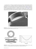
realization of this system is shown in Figure 5.2, along with the details of the control circuit. The simula-
tion of the complete system requires models for the micropump, the microflow sensor, and the electronic
components shown in Figure 5.2. When low-order full-physics models are available for all components
including the fluid flow, the complete system can be simulated using a standard circuit simulator such as

SPICE [Nagel, 1975; Quarles, 1989].
In the absence of macromodels for the micropump and the microflow sensor, the typical approach for
microsystem simulation makes use of lumped-element equivalent circuit descriptions for these devices
[Tilmans, 1996]. However, such an approach has two main limitations:
●
It is suitable only for open-loop systems, where there is no feedback from the output to the input
●
It is applicable only for small-signal conditions
These two limitations arise in the model development process where several assumptions are made in
order to construct the lumped-element equivalent circuits. Therefore, this approach would not be suit-
able when the large-signal behavior of a closed-loop system is of interest.
To address the above problem, we present a coupled circuit/microfluidic device simulator that effi-
ciently couples the discretized Navier–Stokes equations describing a microfluidic device (numerical
model) to the solution of circuit equations. Such a capability is unique in that it allows direct and effi-
cient simulation of microfluidic systems without the need for mapping finite element descriptions into
Integrated Simulation for MEMS 5-5
Fluid in Fluid out
Flow
sensor
Pump
Control
electronics
FIGURE 5.1 Block diagram of a generic microfluidic system. The flow sensor senses the flow rate, which is con-
trolled by the electronic circuit controlling the pump.
© 2006 by Taylor & Francis Group, LLC
equivalent networks [Tilmans, 1996] or analog hardware description languages (AHDLs) [Bielefeld, Pelz,
and Zimmer, 1997].
The rest of this chapter is organized as follows: an overview of coupled circuit and device simulation
is given in section 2, followed by a description of the circuit and fluidic simulators in section 3. The details
of the coupled circuit/fluidic simulator are presented in section 4, and an illustrative example is described

in section 5. Conclusions are provided in section 6.
5.2 Coupled Circuit-Device Simulation
Coupled simulation techniques have previously been used for the simulation of a sensor system [Schroth,
Blochwitz, and Gerlach, 1995]. In this approach, the finite-element program ANSYS [Moaveni, 1999] is
coupled to an electrical simulator PSPICE [Keown, 1997]. Although such an approach has been demon-
strated to work for system simulations, the coupling is not efficient. Special coupling algorithms and
time-stepping schemes are required to enable fast simulation of microsystems. Therefore, a tight coupling
between the circuit and device simulators is necessary for simulation efficiency [Mayaram and Pederson,
1992; Mayaram, Chern, and Yang, 1993].
The coupled circuit-device simulator allows verification of microfluidic systems. It provides accurate
large- and small-signal simulation of systems even in the absence of proper macromodels for the micro-
fluidic devices. On the other hand, the coupled simulator is important for constructing and validating
5-6 MEMS: Introduction and Fundamentals
cA
−
+
cA
−
+
cA
+
_
V
out
Transducer
P
Flow sensor
Heater
T1
Pump

T2
Flow sensor: flow → ∆ T
(Anemometer) ∆ T = T3 – T1
T3
Control circuit : ∆ T → V
out
R2(T3)
R1(T1)
[
[
[
[
Fluid flow
FIGURE 5.2 Realization of the microfluidic system showing the electronic control circuit. The fluid flow deter-
mines the temperature ∆T of the flow sensor. This temperature is transformed by the control electronics into the
voltage Vout, which in turn controls the pump pressure P by a transformation of the voltage to a proportional
pressure.
© 2006 by Taylor & Francis Group, LLC
macromodels. As important effects (such as highly nonlinear or distributed behavior, compressibility, or
slip-flow) are identified, they can be implemented in the macromodels and verified for system simulation
using the coupled simulator. Furthermore, critical devices can be simulated using the full physics-based
numerical models when there are stringent accuracy requirements on the simulated results.
The concept of a coupled circuit and device simulator has proved to be extremely beneficial in the
domain of integrated circuits. Since the first of such simulators, MEDUSA [Engl, Laur, and Dirks, 1982],
became available in the early 1980s, there has been significant work addressing coupled simulation. These
activities have focused on improved algorithms, faster execution speeds, and applications. Commercial
Technology Computer Aided Design (TCAD) vendors also support a mixed circuit-device simulation
capability [Technology Modeling Associates, 1997; Silvaco International, 1995]. Since the computational
costs of these simulators are high, they are not used on a routine basis. However, there are several critical
applications in which these simulators are extremely valuable. These include simulation of Radio

Frequency (RF) circuits [Rotella et al., 1997], single-event-upset simulation of memories [Woodruff and
Rudeck, 1993], simulation of power devices [Ravanelli and Hu, 1991], and validation of nonquasistatic
MOSFET models [Park, Ko, and Hu, 1991].
The coupled circuit-device simulator for microfluidic applications is illustrated in Figure 5.3. This sim-
ulator supports compact models for the electronic components and available macromodels for microflu-
idic devices. In addition, numerical models are available for the microfluidic components that can be
utilized when detailed and accurate modeling is required. As an example, specific components such as
microvalves, micropumps, and micro-flow-sensors are shown in Figure 5.3. The coupling of the circuit and
microfluidic components is handled by imposing suitable boundary conditions on the fluid solver. This
simulator allows the simulation of a complete microfluidic system including the associated control elec-
tronics. The details of the various simulators and coupling methods are described in the sections below.
One of the biggest disadvantages of such an approach is the high computational cost involved. The main
cost comes from solving the three-dimensional time-dependent Navier–Stokes equations in complex geo-
metric domains. Thus, efficient flow solvers are critical to the success of a coupled circuit-micro-fluidic
device simulator. Any performance improvements in the solution of the Navier–Stokes equations directly
translate into a significant performance gain for the coupled simulator.
Integrated Simulation for MEMS 5-7
Designer
Geometry
structure
Circuit
simulator
Compact
models
Macro
models
Numerical
models
Analyses
DC

AC
Transient
BJT
MOSFET
Diode
R
C
Micro
devices
Micro
valve
Pump
Flow
sensor
FIGURE 5.3 The coupled circuit-fluidic device simulator. Microfluidic systems including the control electronics can
be simulated using accurate numerical models for all components.
© 2006 by Taylor & Francis Group, LLC
5.3 Overview of Simulators
The circuit simulator employed here is based on the circuit simulator SPICE3f5 [Quarles, 1989] and the
microfluidic simulator on the code N
εκ
T
α
r [Karniadakis and Sherwin, 1999; Kirby et al., 1999]. A brief
description of the algorithms and software structure of each of these simulators is provided in this section.
5.3.1 The Circuit Simulator: SPICE3
Electrical circuits consist of many components (resistors, capacitors, inductors, transistors, diodes, and inde-
pendent sources) that are described by algebraic and/or differential relations among the components’ cur-
rents and voltages. These relationships are called the branch constitutive relations [Sangiovanni-Vincentelli,
1981]. The circuits also satisfy conservation laws known as the Kirchhoff’s laws; these laws result in alge-

braic equations. Therefore, a circuit is described by a set of coupled nonlinear differential algebraic equa-
tions that are both highly nonlinear and stiff, and this imposes certain limitations on the solution
methods. One of the most commonly used analyses is the time-domain transient analysis. We briefly
describe below the solution approach used for this analysis.
Time discretization: At each time-step of the transient analysis, the time derivatives are replaced by an
algebraic equation using an integration method. Typically, an implicit linear multistep method of the
backward-differentiation type suitable for stiff ODEs is used [Sangiovanni-Vincentelli, 1981]:
ν
Ϸ
α
0
ν
t
n
ϩ
Α
n
kϭ1
α
k
ν
t
nϪk
(5.2)
Linearization: Time discretization yields a system of nonlinear algebraic equations, which are typically
solved by a Newton–Raphson method. The nonlinear components are replaced by linear equivalent mod-
els for each iteration of the Newton’s method
f(
ν
t

n
jϩ1
Ϸ f(
ν
t
n
j
) ϩ ∂ f(
ν
)/∂
ν
|
ν
j
t
n
и (
ν
t
n
jϩ1
Ϫ
ν
t
n
j
) (5.3)
Equation solution: After time discretization and application of Newton’s method a linear system of
equations is obtained at each iteration of the Newton method. These equations are described by
Av

jϩ1
ϭ b (5.4)
where A ∈ ᑬ
nϫn
, v
jϩ1
∈ ᑬ
n
, b ∈ ᑬ
n
, and can be solved by sparse matrix techniques [Kundert, 1990].
The time-domain simulation algorithm can be summarized in the following steps [Sangiovanni-
Vincentelli, 1981]:
1. Read circuit description and initialize data structures.
2. Increment time t
n
ϭ t
nϪ1
ϩ h.
3. Update values of independent sources at t
n
.
4. Predict values of unknown variables at t
n
.
5. Apply integration formula (1) to capacitors and inductors.
6. Apply linearization (2) to nonlinear circuit elements.
7. Assemble linear circuit equations.
8. Solve linear circuit equations.
9. Check convergence. If not converged go to step 6.

10. Estimate local truncation error.
11. Select new time step h; rollback time if truncation error is unacceptable.
12. If t
n
Ͻ t
stop
go to step 3.
5.3.2 The Fluid Simulator: N
εεκκ
T
αα
r
The flow solver corresponds to a particular version of the code N
εκ
T
α
r, which is a general purpose
Computational Fluid Dynamics (CFD) code for simulating incompressible, compressible, and plasma
5-8 MEMS: Introduction and Fundamentals
© 2006 by Taylor & Francis Group, LLC
flows in unsteady three-dimensional geometries. The major algorithmic developments are described in
[Sherwin, 1995] and [Warburton, 1999], and the capabilities are summarized in Figure 5.4. The code uses
meshes similar to standard finite-element and finite-volume meshes consisting of structured or unstruc-
tured grids or a combination of both. The formulation is also similar to those methods, corresponding to
Galerkin and discontinuous Galerkin projections for the incompressible and compressible Navier–Stokes
equations, respectively. Field variables, data, and geometry are represented in terms of hierarchical
(Jacobi) polynomial expansions [Karniadakis and Sherwin, 1999]; both isoparametric and superparamet-
ric representations are employed. These expansions are ordered in vertex, edge, face, and interior (or bub-
ble) modes. For the Galerkin formulation, the required C
0

continuity across elements is imposed by
choosing appropriately the edge (and face in 3D) modes; at low-order expansions this formulation
reduces to the standard finite element formulation. The discontinuous Galerkin is a flux-based formula-
tion, and all field variables have L
2
continuity; at low order this formulation reduces to the standard finite-
volume formulation.
This new generation of Galerkin and discontinuous Galerkin spectral/hp element methods imple-
mented in the code N
εκ
T
α
r does not replace but rather extends the classical finite element and finite
volumes that the CFD practitioners are familiar with [Karniadakis and Sherwin, 1999]. The additional
advantages are that convergence of the discretization and thus solution verification can be obtained with-
out remeshing (h-refinement) and that the quality of the solution does not depend on the quality of the
original discretization. In Figure 5.4 we summarize the major current capabilities of the general code
N
εκ
T
α
r for incompressible, compressible, and even plasma flows. In particular, for microflows both the
compressible and incompressible versions are used. For gas microflows we account for rarefaction by
using velocity-slip and temperature-jump boundary conditions as described in this volume in the chap-
ter by Beskok (see also [Beskok, Karniadakis, and Trimmer, 1996; Beskok and Karniadakis, 1999]). An
extension of the classical Maxwell’s boundary condition is employed in the code in the form
U
g
Ϫ U
w

ϭ (∇U)
w
и nˆ (5.5)
Kn
ᎏ
1 Ϫ bKn
Integrated Simulation for MEMS 5-9
Νεκταr
2d
2.5d
Steady
domain
Steady
domain
Incompressible Navier
–
Stokes
Galerkin
2
d
S
te
a
d
y
d
o
m
a
in

N
a
v
ie
r
–
S
to
k
e
s
D
is
c
o
n
tin
u
o
u
s
G
a
le
r
k
in
E
u
le

r
S
te
a
d
y
d
o
m
a
in
S
in
g
le
flu
id
2
-flu
id
A
L
E
M
h
d
3
d
N
a

v
ie
r
–
S
to
k
e
s
E
u
le
r
S
te
a
d
y
d
o
m
a
in
S
in
g
le
flu
id
A

L
E
M
h
d
ALE
3d
Steady
domain
ALE
2
.5
d
Compress
ible
FIGURE 5.4 Hierarchy of the N
εκ
T
α
r code. Note that “2.5d” refers to a three-dimensional capability with one of
the directions being homogeneous in the geometry. Also, ALE refers to moving computational domains required in
dynamic flow–structure interactions. Gaseous microflows can be simulated by either the compressible or incom-
pressible version depending on the pressure/density variations.
© 2006 by Taylor & Francis Group, LLC
Here we define the Knudsen number Kn ϭ
λ
/L with
λ
the mean free path of the gas molecules and L the
characteristic length scale in the flow. Also, U

g
is the velocity (tangential component) of the gas at the wall,
U
w
is the wall
velocity, and n is the unit normal vector. The constant b is adjusted to reflect the physics of the
p
roblem as we go from the slightly rarefied regime (slip flow)to the transition regime (Kn Ϸ 1) or free
molecular regime (Kn Ͼ 5–10). For b ϭ 0, we recover the classical linear relationship between velocity-slip
and shear stress first proposed by Maxwell. However, for b ϭϪ1we obtain a second-order accuracy
[Beskok and Karniadakis, 1999], and in general for b  0 Equation (5.5) leads to finite slip at the wall
unlike the linear boundary condition (for b ϭ 0) used in most codes. The boundary condition in
Equation (5.5) has been used with success in the entire Knudsen number regime, Kn Ϸ 0–200, [see several
examples in Beskok and Karniadakis (1999)].
One of the key points in obtaining efficiency in simulations of moving domains is the type of dis-
cretization employed in the flow solver. In N
εκ
T
α
r we employ the so-called h-p version of the finite-
element method with spectral Jacobi polynomials as basis functions.Convergence is obtained via a dual path
in this approach, either by increasing the number of elements (h-refinement) or by increasing the order
of the spectral polynomial (p-refinement). In the latter case a faster convergence is obtained without the
need for remeshing. Instead, the number of degrees of freedom is increased in the modal space by increas-
ing the polynomial order (p)while keeping the mesh unchanged. It is, of course, the cost of reconstruct-
ing the mesh that is orders of magnitude higher in time-dependent simulations both in terms of
computer and human time.
Regarding the type of elements (subdomains), N
εκ
T

α
r uses hybrid meshes (i.e., both structured and
unstructured meshes). For example, in three-dimensional simulations a hybrid grid may consist of tetra-
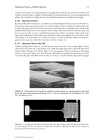
hedra, hexahedra, triangular prisms, and even pyramids. In Figure 5.5 we plot the mesh used in the sim-
ulation of the pump, and in Figure 5.6 we plot the flow field at three different time instances.
In the following section, we briefly describe how we formulate the algorithm for a compatible and effi-
cient flow–structure coupling.
5.3.2.1 Formulation for Flow–Structure Interactions
We consider the incompressible Navier–Stokes equations in a time-dependent domain Ω(t)
u
i,t
ϩ u
j
u
i,j
ϭ Ϫ(p
δ
ij
)
j
ϩ
ν
u
i,jj
ϩ f
i
in Ω(t) (5.6)
u
j,j
ϭ 0 in Ω(t), (5.7)

where
ν
is the viscosity and J
i
is a body force. We assume for clarity homogeneous boundary conditions;
velocity-slip boundary conditions can be included relatively easily in the Galerkin framework as mixed
5-10 MEMS: Introduction and Fundamentals
C
D
Outflow
A
B
Inflow
FIGURE 5.5 Mesh of the pump used in the flow simulator N
εκ
T
α
r. This device was first introduced by [Beskok and
Warburton, 1998] as a mixing device between two microchannels. Here B and C are blocked so the device is operat-
ing as a pump from A to D.
© 2006 by Taylor & Francis Group, LLC
(Robin) boundary conditions. Multiplying Equation (5.6) by test functions and integrating by parts we
obtain
͵
Ω
(t)
ν
i
(u
i,t

ϩ u
j
u
i,j
)dx ϭ ͵
Ω
(t)
ν
i,j
(p
δ
ij
Ϫ
ν
u
i,j
ϩ
ν
i
f
i
)dx (5.8)
The next step is to define the reference system on which time differentiation takes place. This was accom-
plished in [Ho, 1989] by use of the Reynolds transport theorem and by using the fact that the test func-
tion
ν
i
is following the material points. Therefore, its time-derivative in that reference frame is zero,
| x
p

ϭ
ν
i,t
ϩ w
j
ν
i,j
ϭ 0,
where w
j
is a velocity that describes the motion of the time-dependent domain Ω(t); x
p
denotes the mate-
rial point. The final variational statement then becomes
͵
Ω(t)
ν
i
u
i
dx ϩ ͵
Ω(t)
[
ν
i
(u
j
Ϫ w
j
)u

i,j
Ϫ
ν
i
u
i
w
j,j
]dx ϭ ͵
Ω(t)
[
ν
i,j
p
δ
ij
Ϫ
ν ν
i,j
u
i,u
ϩ
ν
i
f
i
]dx (5.9)
d
ᎏ
dt

d
ν
i
ᎏ
dt
Integrated Simulation for MEMS 5-11
FIGURE 5.6 Close-up of the vorticity contours for Re ϭ 30 simulation at the left valve (meshes shown on right
side). Top:
τω
ϭ 0.28 corresponds to the beginning of the suction stage. Start-up vortices due to the motion of the
inlet valve can be identified. Middle:
τω
ϭ 0.72, corresponding to the end of the suction stage. A vortex jet pair is vis-
ible in the pump cavity. Bottom:
τω
ϭ 0.84, corresponding to early ejection stage. Further evolution of the vortex jet
and the start-up vortex of the exit valve can be identified. (Reprinted with permission from A. Beskok).
© 2006 by Taylor & Francis Group, LLC
This is the ALE formulation of the momentum equation. It reduces to the familiar Eulerian and
Lagrangian form by setting w
j
ϭ 0 and w
j
ϭ u
j
respectively. However, w
j
can be chosen arbitrarily to min-
imize the mesh deformation. We discuss this algorithm next.
5.3.2.2 Grid Velocity Algorithm

The grid velocity is arbitrary in the ALE formulation, and therefore great latitude exists in the choice of
technique for updating it. Mesh constraints such as smoothness, consistency, and lack of edge crossover,
combined with computational constraints such as memory use and efficiency dictate the update algo-
rithm used. In the current work, we address the problem of solving for the mesh velocity in terms of its
graph theory equivalent problem. Mesh positions are obtained using methods based on a graph theory
analogy to the spring problem. Ver t i c es are treated as nodes,while edges are treated as springs of varying
length and tension. At each time step, the mesh coordinate positions are updated by equilibration of the
spring network. Once the new vertex positions are calculated, the mesh velocity is obtained through dif-
ferences between the original and equilibrated mesh vertex positions.
Specifically, we incorporate the idea of variable diffusivity while maintaining computational efficiency
by avoiding solving full Laplacian equations. The method we use for updating the mesh velocity is a vari-
ation of the barycenter method [Battista, Eades, Tamassia, and Tollis, 1998] and relies on graph theory.
Given the graph G ϭ (V, E ) of element vertices V and connecting edges E,we define a partition V ϭ V
0
ʜ
V
1
ʜ V
2
of V such that V
0
contains all vertices affixed to the moving boundary, V
1
contains all vertices on
the outer boundary of the computational domain, and V
2
contains all remaining interior vertices. To cre-
ate the effect of variable diffusivity, we use the concept of layers.As is pointed in [Lohner and Yang, 1996],
it is desirable for the vertices very close to the moving boundary to have a grid velocity almost equivalent
to that of the boundary. Hence, locally the mesh appears to move with solid movement, whereas far away

from the moving boundary the velocity must gradually go to zero. To accomplish this in our formulation,
we use the concept of local tension within layers to allow us to prescribe the rigidity of our system. Each
vertex is assigned to a layer value that heuristically denotes its distance from the moving boundary.
Weights are chosen such that vertices closer to the moving boundary have a higher influence on the
updated velocity value. To find the updated grid velocity u
g
at a vertex
ν
ʦ V
2
,we use a force-directed
method. Given a configuration as in Figure 5.7, the grid velocity at the center vertex is given by:
u
g
ϭ
Α
deg(
ν
)
iϭ1
α
l
i
u
i
,
Α
deg(
ν
)

iϭ1
α
l
i
ϭ 1,
where deg(
ν
) is the number of edges meeting at the vertex v and
α
l
i
is the lth layer weight associated with
the i-th edge. This is subjected to the following constraints: u
g
ϭ 0(∀
ν
∈ V
1
), and u
g
(∀
ν
∈ V
0
) is pre-
scribed to be the wall velocity. This procedure is repeated for a few cycles following an incomplete iteration
algorithm, over all
ν
∈V
2

.(Hereby incomplete we mean that only a few sweeps are performed and not
full convergence is sought.) Once the grid velocity is known at every vertex, the updated vertex positions
are determined using explicit time-integration of the newly found grid velocities.
An example of the relative speed-up gained following the graph-theory approach versus the classical
approach of employing Poisson solvers to update the grid velocity is shown in Figure 5.8.We have com-
puted the portion of CPU time devoted exclusively to the solver as a function of the spectral order
5-12 MEMS: Introduction and Fundamentals
u
u
u
u
u
2
3
1
4
␣
␣
␣
1
2
4
1
␣
3
1
1
1
FIGURE 5.7 Graph showing vertices with associated velocities and edges with associated weights.
© 2006 by Taylor & Francis Group, LLC

employed in the discretization. The problem we considered involved the motion of a piezoelectric mem-
brane induced by vortex shedding caused by a bluff body in front of the membrane. We see that a two-
to three-orders of magnitude speed-up can be obtained using the graph-based algorithm.
5.3.3 The Structural Simulator
The membrane of the micropump is modeled using the linear string-beam equation as given by the fol-
lowing equation:
ϩ ϩ Ϫ ϭ
(5.10)
where E is the Young’s modulus of elasticity, I is the second moment of inertia, T is the axial tension, F is
the hydrodynamic forcing, R is the coefficient of structural damping, and m is the structural mass per
unit length. In this model, the coefficients are given by the physical parameters of the membrane used
within the pump, and the hydrodynamic forcing on the membrane is provided by N
εκ
T
α
r.
Assume that the membrane lies in the interval [0,L]. For the micropump configuration, we have cho-
sen the boundary conditions y(0) ϭ y(L) ϭ 0, yЉ(0) ϭ yЉ(L) ϭ 0, which correspond to a fixed-hinged
membrane. Equation (5.10) combined with these boundary conditions lends itself to the use of eigen-
function decomposition for the efficient solution of the membrane motion. We begin by transforming
the problem to lie on the interval [0,1] using the linear mapping x ϭ L
ξ
,
ξ
∈ [0,1]. The eigenfunctions of
this system are given by
φ
n
ϭ sin
͙

λ
ෆ
n
ෆ
ξ
;
͙
λ
ෆ
n
ෆ
ϭ (n Ϫ 1)
π
n ϭ 1, 2,… , ϱ
If we assume a solution of the form
y(
ξ
,t) ϭ
Α
N
nϭ1
A
n
(t)
φ
n
(
ξ
),
1

ᎏ
2
F
ᎏ
m
d
2
y
ᎏ
dx
2
T
ᎏ
m
d
4
y
ᎏ
dx
4
EI
ᎏ
m
dy
ᎏ
dt
R
ᎏ
m
d

2
y
ᎏ
dt
2
Integrated Simulation for MEMS 5-13
FIGURE 5.8 Comparison of CPU time for the grid velocity algorithm between the classical approach (Poisson solver)
and the new approach (graph algorithm). In the leftmost column is the order of spectral polynomial approximation.
© 2006 by Taylor & Francis Group, LLC
then by employing the Galerkin method we obtain the following evolution equation for the coefficients
A
n
(t):
ϩ ϩ
΂
λ
n
Ϫ
΃
λ
n
A
n
ϭ ͵
1
0
Fd
ξ
(5.11)
We then solve this evolution equation using the Newmark scheme [Hughes, 1987], which returns the

coefficients for the displacement, velocity, and acceleration of the membrane. This information is then
returned to N
εκ
T
α
r as demonstrated in Figure 5.9.
5.3.4 Differences among Circuit, Fluid, and Solid Simulators
The above descriptions suggest some differences between the various simulators. The key distinguishing
features are:
●
The fluid simulator is computationally more expensive than the structure and circuit simulators.
●
SPICE3 has a reliable error estimation for time discretization. Therefore, arollback in time can be
done if the truncation error is unacceptable. As a result, SPICE3 automatically controls the simula-
tion time step to ensure an acceptable user-specified error. N
εκ
T
α
r is a much more complex code
and does not have an automatic time-step control scheme for coupled fluid–structure simulation.
●
SPICE3 uses implicit numerical integration methods for time-domain simulation. These methods
are efficient for circuit simulation because the circuit equations are stiff. For the fluid solver, how-
ever, explicit methods are simpler to implement and reasonably efficient. For this reason, N
εκ
T
α
r
uses semiimplicit methods for the time domain integration (explicit for the advection terms and
implicit for the diffusion terms of the Navier–Stokes equations), which suffer from the standard

CFL (Courant–Friedrichs–Levy condition for the time step) restrictions. However, the flow time
step is much higher than the electronics time step due to the relevant physical time scales. Also, the
Newmark scheme for the structure is unconditionally stable.
5.4 Circuit-Micro-Fluidic Device Simulation
For coupled circuit-micro-fluidic device simulation, four different physical domains (electrical, structure
mechanical, fluid mechanical, and thermal) must be considered, as shown in Figure 5.10. These domains
are coupled to one another as described below.
In Figure 5.2 four types of coupling can be identified. These are
●
Electromechanical coupling for a piezoelectric actuation of the pump membrane
●
Fluid–structure coupling due to volume displacement of the pump membrane
1
ᎏ
m
T
ᎏ
m
2
EI
ᎏ
mL
4
dA
n
ᎏ
dt
R
ᎏ
m

d
2
A
n
ᎏ
dt
2
5-14 MEMS: Introduction and Fundamentals
Νεκταr
Structural
solver
Hydrodynamic
forces
Structural
displacement,
velocity and
acceleration
FIGURE 5.9 Coupling between N
εκ
T
α
r and the structural solver. N
εκ
T
α
r provides the hydrodynamic force infor-
mation on the membrane. With this information the structural solver calculates the membrane’s response. Structural
displacement, velocity and acceleration are then returned to N
εκ
T

α
r for determining the influence of the structure’s
motion on the fluid.
© 2006 by Taylor & Francis Group, LLC
●
Fluid-thermal coupling because of the thermoresistor cooling in the fluid when an anemometer
type of microflow sensor is used
●
Electrothermal thermoresistor heating due to current flow in the microflow sensor
The overall system can be simulated using different approaches. One approach is a detailed physical
simulation for each coupled domain. Another is the use of lumped-element equivalent circuits, compact,
or macromodels, and/or analog hardware description languages. A third approach is to use a combina-
tion of coupled solvers, compact models, and lumped elements. In this work, we will demonstrate this
third approach.
5.4.1 Software Integration
The interaction of the full system is based on different abstraction levels, using lumped circuit elements,
compact/macromodels, and a direct interconnection of solvers for various domains. The circuit simula-
tor SPICE3 is chosen as the controlling solver for the following reasons:
●
SPICE3 has advanced time-step control.
●
Models for different abstraction levels can be easily implemented in SPICE3.
●
Lumped-element equivalent circuits can be readily simulated.
Relatively simple elements are implemented as lumped elements or compact models. These elements are
electromechanical transducers (piezoelectric actuator) and thermoresistors. Flow sensors are much more
complicated but often the fluid flow around sensors is relatively simple. For example, if the fluid flow in
achannel is fully developed then it has a parabolic profile for the velocity, and thus this profile (compact
model) can be used for the flow sensors as well. It is important to note that these compact models are
parameterized and can be highly nonlinear. These models are obtained by insight gained from detailed

physical level simulations, such as Navier–Stokes simulations, DSMC, and linearized solutions of the
Boltzmann equation [Beskok and Karniadakis, 1999]. The pump can also be described as a lumped ele-
ment [Klein, Matsumoto, and Gerlach, 1998]. However, these lumped-element descriptions are applica-
ble only for small variations in the fluid flow. Usually pumps operate in a nonlinear and nonsmooth
mode of fluid flow with a strong fluid–structure interaction. Therefore, a detailed physical level simula-
tion of the pump is required. A simplification can be made by employing a macromodel of the form
described in Equation (5.1), but here we employ full Navier–Stokes simulations with full dynamics.
For this reason, the following options are used:
●
Electromechanical actuators, thermoresistors, and flow sensors are described as lumped elements
and/or compact models.
●
The pump is modeled at the detailed physical level.
●
All lumped elements and models are implemented in SPICE3.
●
The pump is implemented as a direct SPICE3-N
εκ
T
α
r interconnection (Figure 5.11). SPICE3
transfers the time t
spice
and pressure P for the membrane activation to N
εκ
T
α
r and receives the flow
rate Q and the time t
call

for the next call to N
εκ
T
α
r.
A detailed description of this coupling is provided later.
Integrated Simulation for MEMS 5-15
Electrical
domain
Solid
domain
Fluid
domain
Thermal
domain
FIGURE 5.10 Coupling between the various physical domains.
© 2006 by Taylor & Francis Group, LLC
5.4.2 Lumped-Element and Compact Models for Devices
5.4.2.1 Model for Piezoelectric Transducers
The model for electromechanical coupling with a piezoelectric actuation of the membrane is shown in
Figure 5.12. This model forms the interface between the electrical and mechanical networks. The electrical
characteristics of the piezoelectric actuator are described by the capacitor C. The input voltage Vtrans-
lates into an output pressure P by virtue of the piezoelectric effect with coefficient k. This pressure is an
input argument to N
εκ
T
α
r.The mechanical characteristics of the piezoelectric actuator are coupled with
the mechanical characteristics of the substrate [Klein, 1997; Timoshenko and Woinowsky-Krieger, 1970].
5.4.2.2 Compact Model for Flow Sensor

For an anemometer type flow sensor [Rasmussen and Zaghloul, 1999] shown in Figure 5.13, a macro-
model has been developed in [Mikulchenko, Rasmussen, and Mayaram, 2000]. This macromodel (Figure
5.14) is based on neural networks trained using data from detailed physical simulations.
The inputs to the neural network are the flow velocity U and the vector of geometrical and physical
parameters Θ.The results from this model are in good agreement with the simulated data for a large
range of parameters [Mikulchenko, Rasmussen, and Mayaram, 2000].
The dynamic macromodel is incorporated in SPICE3 by coupling it with a sensor circuit and a model
for thermoresistors for the heater and sensors as shown in Figure 5.15. Based on the fluid flow rate the
thermoresistor temperatures T1, T2, and T3 change, which in turn alters the resistance values and the
sensing-circuit currents and voltages.
5.4.3 Effective Time-Stepping Algorithms
In general, the flow solver can be N
εκ
T
α
r implemented as one big model in SPICE3. This is accomplished
by N
εκ
T
α
r from SPICE3 for each Newton iteration. However, such a coupling is extremely inefficient
5-16 MEMS: Introduction and Fundamentals
Spice
Νεκταr
P,t
spice
Q,t
call
Pump model
FIGURE 5.11 The SPICE3–N

εκ
T
α
r interaction for the pump microsystem of Figure 5.2.SPICE3 provides the time
t
spice
and pressure P for the membrane actuation to N
εκ
T
α
r. N
εκ
T
α
r transfers the flow rate Q at time t
call
for the next
call of N
εκ
T
α
r by SPICE3.
P = kv
C
v
Membrane
Circuit
FIGURE 5.12 Lumped model for piezoelectric actuation. The voltage V is transformed into a pressure P that is used
to activate the membrane of the pump.
© 2006 by Taylor & Francis Group, LLC

because a call to N
εκ
T
α
r is computationally very expensive. Furthermore, the time scales and nonlinearities
are extremely different for the circuit and fluidic devices. If one considers only the circuit element, then
a SPICE3 simulation results in nonuniform time steps and several Newton iterations for each time step.
Typical time constants for circuits are of the order of 10
Ϫ12
…10
Ϫ6
seconds. On the other hand, fluidic
devices have a typical time constant of the order 10
Ϫ4
…10
Ϫ1
seconds.
Integrated Simulation for MEMS 5-17
FIGURE 5.13 Structure of an anemometer-type flow sensor (thermocouple). This sensor is made up of a heating
element and two sensing elements. The temperature difference between the sensors is used to measure the flow.
U
R
T
ss0
T
ss
C T
Θ
␻
Steady-state nominal model Dynamic extension

FIGURE 5.14 Dynamic macromodel for the flow sensor. The steady-state solution T
SS0
corresponds to a nominal
power for the heat source
χ
. The neural network output T
SS0
is a multivariate function of the flow velocity U and the
vector of geometrical and physical parameters Θ. T
SS
is a linear function of the heat source
χ
and T
SS0
.
R1
R2
R3
T1 T2 T3
i
R2
i
R3
i
R1
i
R2
2
R2
U

Sensor macromodel
Circuit
FIGURE 5.15 Macromodel implementation in SPICE3. Based on the fluid flow rate the thermoresistor tempera-
tures T1, T2, and T3 change, which in turn alters the resistance values and the sensing-circuit currents and voltages.
© 2006 by Taylor & Francis Group, LLC
This property can be exploited to improve simulation performance by calling N
εκ
T
α
r only at some of
the circuit time points following a subcycling type algorithm. Between these time points, the N
εκ
T
α
r
outputs can be modeled as constant values. Further improvement in performance is possible by taking
into account the usage of semiexplicit methods for fluid simulation. In this case, the flow rate Q
n
for time
point t
n
is calculated by the explicit scheme: Q
n
ϭ F(P
nϪ1
,V
nϪ1
,t
n
), where P is the vector of the pressure at

mesh points, and V is the vector of velocities at mesh points. For the SPICE3 N
εκ
T
α
r interaction
described earlier, the important quantities are the distributed pressure P for the pump membrane and the
flow rate Q
n
. This functional relationship can be expressed as follows: Q
n
ϭ f(P
nϪ1
,Q
nϪ1
,t
n
).
Based on this observation, an efficient time-stepping scheme is obtained as shown in Figure 5.16. Here,
time is plotted on the horizontal axis, and the SPICE3 iterations are plotted on the vertical axis; t
S,k
and
t
N,k
are the SPICE3 and N
εκ
T
α
r time points, respectively. N
εκ
T

α
r selects a time step h
N,i
ϭ t
N,i
Ϫ t
N,iϪ1
independent of SPICE3, based on the Courant number (CFL) constraint for convection. The N
εκ
T
α
r
time points t
N,i
are used as synchronization time points with SPICE3, whereby t
N,i
ϭ t
S,k
. The flow rate Q
has a constant value between these synchronization time points. The membrane pressure p
j,k
is calculated
as a function of the circuit behavior for each SPICE3 call at time t
S,k
and iteration j. The pressure P
i
ϭ p
M,k
at the final SPICE3 iteration M, for a synchronization time point t
S,k

ϭ t
N,i
, is an input to N
εκ
T
α
r. A
N
εκ
T
α
r call is made at t
N,i
and a new value of Q is computed using the relation Q
iϩ1
ϭ f (P
i
,Q
i
,t
N,iϩ1
). This
value is then used for the next N
εκ
T
α
r time point, t
N,iϩ1
.
5-18 MEMS: Introduction and Fundamentals

Nεκταr call Nεκταr call Nεκταr call
P
0
=p
2,0
P
1
=p
4,2
P
2
=p
2,5
Q
1
=f(P
0
,Q
0
,t
N1
) Q
2
=f (P
1
,Q
1
,t
N2
) Q

3
=f (P
2
,Q
2
,t
N 3
)
Spice
iteration
p
4,2
Q
1
p
3,1
Q
0
Q
1
p
2,0
Q
0
p
2,1
Q
0
p
2,2

Q
1
p
2,5
Q
1
p
1,0
Q
0
p
1,1
Q
0
p
1,2
Q
1
p
1,3
Q
1
p
1,5
Q
2
p
0,0
Q
0

p
1,0
Q
0
p
0,2
Q
1
p
0,3
Q
1
p
0,5
Q
2
t
S0
t
S1
t
S2
t
S3
t
S4
t
S5
Time
h

S,1
h
N,1
t
N0
t
N1
t
N2
p
3,2
FIGURE 5.16 The time-stepping scheme for SPICE3 N
εκ
T
α
r coupling. T
s,k
and t
N,k
are the SPICE3 and N
εκ
T
α
r
time points respectively. Q
i
is a constant value for each SPICE3 iteration and at each SPICE3 time point between the
N
εκ
T

α
r time points t
N,i
and t
N,iϩ1
. The membrane pressure p
j,k
is calculated as a function of the circuit behavior for
each SPICE3 call at time T
s,k
and iteration j. SPICE3 selects time points based on a local truncation error estimate and
synchronizes with N
εκ
T
α
r at all N
εκ
T
α
r time points. The pressure p
i
for the final SPICE3 iteration at the synchro-
nization time point T
s,k
ϭ t
N,i
is used as an input to N
εκ
T
α

r. N
ε
T
α
r call is made at t
N,i
, and a new value of Q is com-
puted for the next N
εκ
T
α
r time point.
© 2006 by Taylor & Francis Group, LLC
The main features of this time stepping scheme can be summarized as follows:
●
N
εκ
T
α
r is called from SPICE3.
●
The timestep for SPICE3 is much smaller than the timestep for N
εκ
T
α
r.
●
N
εκ
T

α
r specifies the next synchronization time point.
From this, it can be concluded that the number of N
εκ
T
α
r calls are the same as that of stand-alone N
εκ
T
α
r.
This is the best possible situation in terms of efficiency for the coupled SPICE3–N
εκ
T
α
r simulation.
5.5 Demonstrations of the Integrated Simulation Approach
5.5.1 Microfluidic System Description
A microliquid dosing system is used as an illustrative example. This system is made up of a micropump,
a flow sensor and an electronic control circuit. The electronic circuit adjusts the pump flow rate. A sim-
plified simulation circuit is shown in Figure 5.17.
In this system, the flow rate Q determines the flow sensor velocity U for a given set of geometry param-
eters (h, d, wsens). Based on the fluid flow rate, the thermoresistor temperatures T1, T2, and T3 change,
which in turn alters the resistance values R1(T1), R2(T2), and R3(T3). The resistances R1(T1) and
R3(T3) are included in a Wheatstone-bridge arrangement with two fixed resistors R4 and R5. The volt-
age difference V
R3(T3)
Ϫ V
R1(T1)
is directly proportional to the temperature difference T3 Ϫ T1. This volt-

age difference is linearly transformed to the output voltage Vout by an operational amplifier with a
controlled gain. This output voltage determines the pressure P, which activates the pump membrane and
changes the flow rate Q. The thermoresistor of the heater (R2) is activated by the control electronics that
maintain a constant heater temperature.
Integrated Simulation for MEMS 5-19
χ=I
R2
2
R2
R2(T2)
T2
P
R1(T1)
T3
R3(T3)
T1
Vdd
R4 R5
Vout
Piezo-
electric
activator
model
Microflow sensor macromodel
P
Inlet
Pump distributed model
QOutlet
Membrane
V

R2
Heater power
control circuit
FIGURE 5.17 Description of the complete system for simulation. The pump flow rate Q determines the flow sen-
sor velocity U. This yields the temperatures for the sensor thermoresistors. The difference between the resistance val-
ues R1(T1) and R3(T3) is transformed into the voltage V
out
by the control electronics, which are used to control the
pressure P for the pump membrane. This, in turn, determines the flow rate Q.
© 2006 by Taylor & Francis Group, LLC
5-20 MEMS: Introduction and Fundamentals
0 0.1 0.2 0.3 0.4
0
5
10
× 10
6
Time (s)
Pressure P (Pa)
0 0.1 0.2 0.3 0.4
0
0.005
0.01
Time (s)
Velocity U (m/s)
0 0.1 0.2 0.3 0.4
0
50
100
Time (s)

V
out
(V)
FIGURE 5.18 External pressure for the pump membrane, inlet velocity for the microflow sensor, and the amplifier
output voltage for the simulation of the microfluidic system as a function of time.
0 0.02 0.04 0.06 0.08 0.1
0
5
10
15
20
25
Velocit
y
U
(
m/s
)
∆T (°K)
FIGURE 5.19 Flow sensor characteristics and its region of operation. A small change in velocity results in a large
change in ∆T, the difference of the upstream and downstream sensor temperatures.
© 2006 by Taylor & Francis Group, LLC
5.5.2 SPICE3–N
εεκκ
T
αα
r Integration
As mentioned earlier, N
εκ
T

α
r is embedded as a subroutine in SPICE3. The interaction with SPICE3 is by
means of the model code and the simulation engine. Synchronization time points are determined by
N
εκ
T
α
r and used by the SPICE3 transient analysis engine. The pump is modeled as a SPICE3 element
with N
εκ
T
α
r being the underlying simulation engine. The other elements in the circuit are described by
lumped element descriptions and/or compact models.
5.5.3 Simulation Results
The simulation results from the coupled simulator are presented in Figure 5.18.In this simulation, one can
determine the pressure on the pump membrane, the flow velocity,and the output control voltage as a func-
tion of time for various component parameters. As an example, consider the microflow sensor whose char-
acteristics are shown in Figure 5.19.For the given range of flow velocity, the temperature difference
between the upstream and downstream sensor temperatures is in the range 12–17°K. This simulation
required approximately 5 minutes of CPU time on a 300MHz Pentium II processor. Thus, the coupled
simulator is reasonably efficient and provides valuable information to the system for device developers.
5.6 Summary and Discussion
Coupled-domain simulation is necessary in MEMS applications as many different physical phenomena
are present and different processes are taking place simultaneously. Depending on the specific application
(e.g., a microsensor versus a microactuator or a more complex system), some aspects of the device need
to be simulated in detail at high resolution while others need to be accounted for by a low-dimensional
description. Nonlinear macromodels are a possibility, but they are inadequate for the microfluidic sys-
tem, which is typically highly unsteady and nonlinear. In addition, in the microdomain certain nonstan-
dard flow features have to be modeled accurately, such as velocity-slip or temperature-jump in gas flows,

viscous electrokinetic effects in liquid flows, and particle trajectories in particulate flows. To this end, we
have developed the code that can simulate flows in the microdomains and macrodomains both for liq-
uids and for gases. In addition, it includes a library of linear and nonlinear structures, such as beams,
membranes, and cables.
For the coupled-domain simulation, the main driver program is SPICE3, a popular code for circuit
simulation. In this paper, a coupled circuit and microfluidic device simulator was presented. The resulting
simulator allows simulation of a complete microfluidic system in which thermal, flow, structural, and
electrical domains are integrated. The coupling of these simulators was described and demonstrated for
a microliquid dosing system. The integrated simulator can be utilized for parametric studies and optimal
design of microfluidic systems.
The integration of different simulators required for complete MEMS simulations is a difficult problem
with challenges well beyond software integration. It involves disparate temporal and spatial scales lead-
ing to great stiffness and inefficiencies, new physical assumptions and approximations for some of the
components, issues of numerical stability, staggered time-marching procedures, new fast solvers for cou-
pled problems, and optimization and control algorithms. Most of the mature algorithms from single dis-
ciplines are inefficient in this context, so new methods are required in order to produce a new generation
of simulation algorithms for MEMS devices. In this chapter, we have demonstrated that this is possible
by coupling two accurate codes and resolving at least at some level some of these coupling issues.
However, significant improvements can be made for specific devices. For example, for the membrane-
driven micropump presented here, convergence of the coupling algorithm could be accelerated by
inspecting the time-dependent mass-conservation equation every SPICE time step and obtaining a new
estimate of flow from
Q
new
ϭ Q
old
ϩ
∆V
ᎏ
∆t

Integrated Simulation for MEMS 5-21
© 2006 by Taylor & Francis Group, LLC
where ∆V is the change in volume due to the change in the membrane position, and ∆t is the time
between two consecutive SPICE calls. This requires solving for the structure only but not necessarily for
the entire flow field, which is the most computationally intensive task. The structure solver is very fast and
can be called as often as necessary without a serious computational overhead.
Acknowledgments
This work is supported in part by DARPA under agreement number F30602-98-2-0178. We would like to
thank Prof. A. Beskok for many useful suggestions regarding this work.
References
Allen, M., and Tildesley, D. (1994) Computer Simulation of Liquids, Clarendon Press, Oxford.
Aluru, N. (1999) “A Reproducing Kernel Particle Method for Meshless Analysis,” Comput. Mech. 23,
pp. 324–38.
Aluru, N., and White, J. (1996) “Direct-Newton Finite-Element/Boundary-Element Technique for Micro-
Electro-Mechanical Analysis,” in Tech. Digest: Solid-State Sensor and Actuator Workshop, Hilton
Head Is. SC, pp. 54–57.
Aluru, N.R., and White, J. (1997) “An efficient numerical technique for electromechanical simulation of
complicated microelectromechanical structures,” Sensors and Actuators, A-58, pp. 1–11.
Battista, G.D., Eades, P., Tamassia, R., and Tollis, I. (1998) Graph Drawing, Prentice Hall, Englewood Cliffs, NJ.
Beskok, A., and Karniadakis, G.E. (1999) “A Model for Flows in Channels, Pipes and Ducts at Micro- and
Nano-Scales,” J. Microscale Thermophys. Eng. 3, pp. 43–77.
Beskok, A., Karniadakis, G.E., and Trimmer, W. (1996) “Rarefaction and Compressibility Effects in Gas
Microflows,” J. Fluids Eng. 118, p. 448.
Bielefeld, J., Pelz, G., and Zimmer, G. (1997) “AHDL-Model of a 2D Mechanical Finite-Element Usable
for Microelectro-Mechanical Systems,” in BMAS’97, pp. 177–81, IEEE, Washington, D.C.
Bird, G. (1994) Molecular Gas Dynamic and the Direct Simulation of Gas Flows, Oxford Science
Publications, Oxford.
Engl, W.L., Laur, R., and Dirks, H.K. (1982) “MEDUSA-A Simulator for Modular Circuits,” IEEE Trans.
Comput. Aid. Design 1, April, pp. 85–93.
Freeman, D., Aranyosi, A., Gordon, M., and Hong, S. (1998) “Multidimensional Motion Analysis of

MEMS Using Computer Microvision,” in Solid-State Sensor and Actuator Workshop, Hilton Head
Is., S.C., June 1998, pp. 150–55.
Gabbay, L.D. (1998) Computer Aided Macromodeling for MEMS, Ph.D. thesis, Department of Electrical
Engineering and Computer Science, Massachusetts Institute of Technology.
Gad-El-Hak, M. (1999) “The Fluid Mechanics of Microdevices,” J. Fluids Eng. 12(1), pp. 5–33.
Gilbert, J.R. et al. (1993) “Implementation of a MEMCAD System for Electrostatic and Mechanical
Analysis of Complex Structures from Mask Descriptions,” Proc. IEEE Workshop on
Microelectromechanical Systems, MEMS’93, Ft. Lauderdale, February 1993, pp. 207–12.
Hadjiconstantinou, N. (1999) “Hybrid Atomistic-Continuum Formulations and the Moving Contact-
Line Problem,” J. Comp. Phys. 154, pp. 245–65.
Ho, C M., and Tai, Y C. (1998) “Micro-Electro-Mechanical Systems (MEMS) and Fluid Flows,” Annu.
Rev. Fluid Mech. 30, pp. 579–612.
Ho, L W. (1989) A Legendre Spectral Element Method for Simulation of Incompressible Unsteady Free-
Surface Flows, Ph.D. thesis, Department of Mechanical Engineering, Massachusetts Institute of
Technology.
Hughes, T.J.R. (1987) The Finite Element Method, Prentice-Hall, Englewood Cliffs, New Jersey.
Hung, E.S., Yang, Y J., and Senturia, S. (1997) “Low-Order Models for Fast Dynamical Simulations of
MEMS Microstructures,” in Transducers’97, June 1997, pp. 1101–4, IEEE, Chicago.
5-22 MEMS: Introduction and Fundamentals
© 2006 by Taylor & Francis Group, LLC
Karniadakis, G.E., and Sherwin, S.J. (1999) “Spectral/hp Element Methods for CFD,” Oxford University
Press, Oxford.
Keown, J. (1997) Microsim PSPCE and Circuit Analysis, 3rd ed., Prentice Hall, London.
Kirby, R.M., Warburton, T.C., Sherwin, S.J., Beskok, A., and Karniadakis, G.E. (1999) “The N
εκ
T
α
r Code:
Dynamic Simulations with Remeshing,” Second International Conference on Computational
Technologies for Fluid/Thermal/Chemical Systems with Industrial Applications, August 1–5.

Klein, A., and Gerlach, G. (1997) “Modelling of Piezoelectric Bimorph Structures Using an Analog Hardware
Description Language,” in Second International Conference on the Simulation and Design of
Microsystems and Microstructures (MICROSIM’97), Lausanne (Switzerland), September in Adey
and Renaud “Microsim II-Simulation and Design of Microsystems and Microstructures”,
Computational Mechanics Publications, Southampton, UK/Boston, USA, 1998, pp. 229–38.
Klein, A., Matsumoto, S., and Gerlach, G. (1998) “Modeling and Design Optimization of a Novel
Micropump,” in First International Conference on Modeling and Simulation of Microsystems,
Semiconductors, Sensors and Actuators, 6–8 April, Santa Clara, California, pp. 506–11.
Koplik, J., and Banavar, J. (1995) “Continuum Deductions from Molecular Hydrodynamics,” Annu. Rev.
Fluid Mech. 27, pp. 257–92.
Kundert, K.S. (1990) “Sparse-Matrix Techniques and Their Application to Circuit Simulation,” in Circuit
Analysis, Simulation and Design, North-Holland Co, New York, NY.
Lo, N.R. et al. (1996) “Parameterized Layout, Synthesis, Extraction, and SPICE Simulation for MEMS,”
ICASE ’96, pp. 481–84.
Lohner, R., and Yang, C. (1996) “Improved ALE Mesh Velocities for Moving Bodies,” Comm. Num. Meth.
Eng., Phys. 12, pp. 599–608.
Mayaram, K., Chern, J., and Yang, P. (1993) “Algorithms for Transient Three-Dimensional Mixed-Level
Circuit and Device Simulation,” IEEE Trans. Comput. Aid. Design 12, pp. 1726–33.
Mayaram, K., and Pederson, D.O. (1987) “Analysis of MOS Transformer-Coupled Oscillators”, IEEE
J. Solid-State Circuits, 22, pp. 1155–62.
Mayaram, K., and Pederson, D.O. (1992) “Coupling Algorithms for Mixed-Level Circuit and Device
Simulation,” IEEE Trans. Comput. Aid. Design 11, pp. 1003–12.
Mikulchenko, O., Rasmussen, A., and Mayaram, K. (2000) “A Neural Network Based Macromodel of
Microflow Sensors,” Proc. of MSM2000, NSTI (Nano Science and Technology Institute),
pp. 540–43, Cambridge, Massachusetts.
Moaveni, S. (1999) Finite Element Analysis: Theory and Application with ANSYS, Prentice Hall, New Jersey.
Nagel, L.W. (1975) “SPICE2: A Computer Program to Simulate Semiconductor Circuits,” Tech. Rep. No.
UCB/ERL M520, Electronics Research Lab., Univ. of California, Berkeley.
Park, H.J., Ko, P.K., and Hu, C. (1991) “A Charge Conserving Non-Quasi-Static (NQS) Model for SPICE
Transient Analysis,” IEEE Trans. Comput. Aid. Design 10, pp. 629–42.

Quarles, T.L. (1989) “The SPICE3 Implementation Guide,” Tech. Rep. No. UCB/ERL M89/44, Electronics
Research Lab., Univ. of California, Berkeley.
Rasmussen, A., and Zaghloul, M.E. (1999) “The Design and Fabrication of Microfluidic Flow Sensors,” in
Proc. ISCAS–99, pp. 136–39, IEEE, Orlando, FL.
Ravanelli, E., and Hu, C. (1991) “Device-Circuit Mixed Simulation of VDMOS Charge Transients,” Solid
State Electron. 34, pp. 1353–60.
Rotella, F.M., Troyanovsky, B., Yu, Z., Dutton, R., and Ma, G. (1997) “Harmonic Balance Device Analysis
of an LDMOS RF Power Amplifier with Parasitics and Matching Network,” in SISPAD–97,
pp. 157–59, IEEE, Picataway, NJ.
Sangiovanni-Vincentelli, A.L. (1981) “Circuit Simulation,” in Computer Design Aids for VLSI Circuits,
Sijthoff and Noordhoff, pp. 19–113, Boston, MA.
Schroth, A., Blochwitz, T., and Gerlach, G. (1995) “Simulation of a Complex Sensor System Using Coupled
Simulation Programs,” in Transducers ’95, pp. 33–35, IEEE, Stockholm, Sweden.
Senturia, S., Aluru, N., and White, J. (1997) “Simulating the Behavior of MEMS Devices: Computational
Methods and Needs,”IEEE Computational Science & Engineering, vol. 4(1) January–March, pp. 30–43.
Integrated Simulation for MEMS 5-23
© 2006 by Taylor & Francis Group, LLC