The MEMS Handbook Introduction & Fundamentals (2nd Ed) - M. Gad el Hak Part 5 ppsx

and liquids go through multiple collisions at a given instant, making the treatment of the intermolecular
collision process more difficult. The dilute gas approximations, along with molecular chaos and equipar-
tition of energy principles, lead us to the well established kinetic theory of gases and formulation of the
Boltzmann transport equation starting from the Liouville equation. The assumptions and simplifications
of this derivation are given in Vincenti and Kruger (1977) and Bird (1994).
Momentum and energy transport in the bulk of the fluid happen with intermolecular collisions, as
does settling to a thermodynamic equilibrium state. Hence, the time and length scales associated with the
intermolecular collisions are important parameters for many applications. The distance traveled by the
molecules between the intermolecular collisions is known as the mean free path. For a simple gas of hard-
sphere molecules in thermodynamic equilibrium, the mean free path is given in the following form [Bird,
1994]:
λ
ϭ (2
1/2
π
d
2
m
n)
Ϫ1
(6.6)
The gas molecules are traveling with high speeds proportional to the speed of sound. By simple consid-
erations, the mean-square molecular speed of the gas molecules is given by [Vincenti and Kruger, 1977]:
͙
C
ෆ
ෆ
2
ෆ
ϭ
Ί

๶
ϭ
͙
3R
ෆ
T
ෆ
(6.7)
where R is the specific gas constant. For air under standard conditions, this corresponds to 486m/sec. This
value is about 3 to 5 orders of magnitude larger than the typical average speeds obtained in gas
microflows. (The importance of this discrepancy will be discussed in Section 6.2.3.) In regard to the time
scales of intermolecular collisions, we can obtain an average value by taking the ratio of the mean free
path to the mean-square molecular speed. This results in t
c
ഡ 10
Ϫ10
for air under standard conditions.
This time scale should be compared to a typical microscale process time scale to determine the validity of
the thermodynamic equilibrium assumption.
So far we have identified the vast number of molecules and the associated time and length scales for
gas flows. That it is possible to lump all of the microscopic quantities into time- and/or space-averaged
macroscopic quantities, such as fluid density, temperature, and velocity. It is crucial to determine the
limitations of these continuum-based descriptions; in other words:
●
How small should a sample size be so that we can still talk about the macroscopic properties and
their spatial variations?
●
At what length scales do the statistical fluctuations become significant?
It turns out that a sampling volume that contains 10,000 molecules typically results in 1% statistical fluc-
tuations in the averaged quantities [Bird, 1994]. This corresponds to a volume of 3.7 ϫ 10

−22
m
3
for air at
standard conditions. If we try to measure an “instantaneous” macroscopic quantity such as velocity in a
three-dimensional space, one side of our sampling cube will typically be about 72 nm. This length scale
is slightly larger than the mean free path of air
λ
under standard conditions. Therefore, in complex micro-
geometries where three-dimensional spatial gradients are expected, the definition of instantaneous macro-
scopic values may become problematic for Kn Ͼ 1. If we would like to subdivide this domain further to
obtain an instantaneous velocity distribution, the statistical fluctuations will be increased significantly as
the sample volume is decreased. Hence, we may not be able to define instantaneous velocity distribution
in a 72nm
3
volume. On the other hand, it is always possible to perform time or ensemble averaging of the
data at such small scales. Hence, we can still talk about a velocity profile in an averaged sense.
To describe the statistical fluctuation issues further, we present in Figure 6.2 the flow regimes and the
limit of the onset of statistical fluctuations as a function of the characteristic dimension L and the nor-
malized number density n/n
o
. The 1% statistical scatterline is defined in a cubic volume of side L, which con-
tains approximately 10,000 molecules. Using Equation (6.5), we find that L/
δ
Ϸ 20 satisfies this
condition approximately, and the 1% fluctuation line varies as (n/n
o
)
Ϫ1/3
. Under standard

conditions, 1% fluctuation is observed at L ϭ 72 nm, and the Knudsen number based on this value is
Kn Ϸ 1. Figure 6.2 also shows the continuum, slip, transitional, and free molecular flow regimes for air at
3P
ᎏ
ρ
Molecular-Based Microfluidic Simulation Models 6-5
© 2006 by Taylor & Francis Group, LLC
273 K and at various pressures. The mean free path varies inversely with the pressure. Hence, at isother-
mal conditions, the Knudsen number varies as (n/n
o
)
Ϫ1
. The fundamental question of dynamic similar-
ity of low-pressure gas flows to gas microflows under geometrically similar and identical Knudsen, Mach,
and Reynolds number conditions can be answered to some degree by Figure 6.2. Provided that there are
no unforeseen microscale-specific effects, the two flow cases should be dynamically similar. However, a
distinction between the low-pressure and gas microflows is the difference in the length scales for which
the statistical fluctuations become important.
It is interesting to note that for low-pressure rarefied gas flows the length scales for the onset of signifi-
cant statistical scatter correspond to much larger Knudsen values than do the gas microflows. For example,
Kn ϭ 1.0 flow obtained at standard conditions in a 72 nm cube volume permits us to perform one instan-
taneous measurement in the entire volume with 1% scatter. However, at 100 pascal pressure and 273 K
temperature, Kn ϭ 1.0 flow corresponds to a length scale of 65 mm. For this case, 1% statistical scatter in
the macroscopic quantities is observed in a cubic volume of side 0.72 µm, allowing about 90 pointwise
instantaneous measurements. This is valid for instantaneous measurements of macroscopic properties in
complex three-dimensional conduits. In large-aspect-ratio microdevices, one can always perform spanwise
averaging to define an averaged velocity profile. Also, for practical reasons one can also define averaged
macroscopic properties either by time or ensemble averaging (such examples are presented in Section 6.2.4).
6.2.2 An Overview of the Direct Simulation Monte Carlo Method
In this section, we present the algorithmic details, advantages, and disadvantages of using the direct sim-

ulation Monte Carlo algorithm for microfluidic applications. The DSMC method was invented by Graeme
6-6 MEMS: Introduction and Fundamentals
L (microns)
Kn = 1.0
Kn = 10
L/

= 20
Dilute gas
Dense gas
Kn = 0.1
Kn = 0.01
Slip
flow
Transitional
flow
Free
molecular
flow
Continuum
flow
Navier−Stokes
equations
10
3
10
2
10
1
10

0
10
-1
10
-2
10
-3
10
-4
10
-3
10
-2
10
-1
n/n
0
10
0
10
1
10
2
FIGURE 6.2 Limit of approximations in modeling gas microflows. L is the characteristic length, n/n
o
is the number
density normalized with the corresponding standard conditions. The lines that define the various Knudsen regimes
are based on air at isothermal conditions (T ϭ 273 K). The L/
δ
ϭ 20 line corresponds to the 1% statistical scatter in

the macroscopic properties. The area below this line experiences increased statistical fluctuations.
© 2006 by Taylor & Francis Group, LLC
A. Bird (1976, 1994). Several review articles about the DSMC method are currently available [Bird 1978,
1998; Muntz, 1989; Oran et al., 1998]. Most of these articles present an extended review of the DSMC
method for low-pressure rarefied gas flow applications, with the exception of Oran et al. (1998), who also
address microfluidic applications.
The previous section describes molecular magnitudes and associated time and length scales. Under
standard conditions in a volume of 10 µm
3
, there are about 2.69 ϫ 10
10
molecules. A molecular-based
simulation model that can compute the motion and interactions of all these molecules is not possible.
The typical DSMC method uses hundreds of thousands or even millions of simulated molecules or par-
ticles that mimic the motion of real molecules.
The DSMC method is based on splitting the molecular motion and intermolecular collisions by choos-
ing a time step less than the mean collision time and tracking the evolution of this molecular process in
space and time. For efficient numerical implementation, the space is divided into cells similar to the
finite-volume method. The DSMC cells are chosen proportional to the mean free path
λ
.In order to
resolve large gradients in flow with realistic (physical) viscosity values, the average cell size should be
∆x
c
ഡ
λ
/3 [Oran et al., 1998]. The time- and cell-averaged molecular quantities are obtained as the
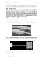
macroscopic values at the cell centers. The DSMC involves four main processes: motion of the particles,
indexing and cross-referencing of particles, simulation of collisions, and sampling of the flow field. The
basic steps of a DSMC algorithm are given in Figure 6.3.

The first process involves motion of the simulated molecules during a time interval of ∆t. Because the
molecules will go through intermolecular collisions, the time step for simulation chosen is smaller than
the mean collision time ∆t
c
. Once the molecules are advanced in space, some of them will have gone
through wall collisions or will have left the computational domain through the inflow–outflow bound-
aries. Hence, the boundary conditions must be enforced at this level, and the macroscopic properties along
the solid surfaces must be sampled. This is done by modeling the surface molecule interactions by applying
the conservation laws on individual molecules rather than using a velocity distribution function that is
commonly utilized in the Boltzmann algorithms. This approach allows inclusion of many other physical
processes, such as chemical reactions, radiation effects, three-body collisions, and ionized flow effects,
without major modifications to the basic DSMC procedure [Oran et al., 1998]. However, a priori knowl-
edge of the accommodation coefficients must be used in this process. Hence, this constitutes a weakness
of the DSMC method similar to the Navier–Stokes-based slip and even Boltzmann equation-based sim-
ulation models. The following section discusses this issue in detail.
The second process is the indexing and tracking of the particles. This is necessary because the mole-
cules might have moved to new cell locations during the first stage. The new cell location of the mole-
cules is indexed, and thus the intermolecular collisions and flow field sampling can be handled accurately.
This is a crucial step for an efficient DSMC algorithm. The indexing, molecule tracking, and data struc-
turing algorithms should be carefully designed for the specific computing platforms, such as vector super
computers and workstation architectures.
The third step is simulation of collisions via a probabilistic process. Because only a small portion of the
molecules is simulated and the motion and collision processes are decoupled, probabilistic treatment
becomes necessary. A common collision model is the no-time-counter technique of Bird (1994) that is
used in conjunction with the subcell technique where the collision rates are calculated within the cells and
the collision pairs are selected within the subcells. This improves the accuracy of the method by main-
taining the collisions of the molecules with their closest neighbors [Oran et al., 1998].
The last process is the calculation of appropriate macroscopic properties by the sampling of molecular
(microscopic) properties within a cell. The macroscopic properties for unsteady flow conditions are obtained
by the ensemble average of many independent calculations. For steady flows, time averaging is also used.

6.2.3 Limitations, Error Sources, and Disadvantages of the DSMC Approach
Following the work of Oran et al., (1998), we identify several possible limitations and error sources within
a DSMC method.
Molecular-Based Microfluidic Simulation Models 6-7
© 2006 by Taylor & Francis Group, LLC
1. Finite cell size: the typical DSMC cell should be about one-third of the local mean free path. Values
of cell sizes larger than this may result in enhanced diffusion coefficients. In DSMC, one cannot
directly specify the dynamic viscosity and thermal conductivity of the fluid. The dynamic viscosity
is calculated via diffusion of linear momentum. Breuer et al. (1995) performed one-dimensional
Rayleigh flow problems in the continuum flow regime and showed that for cell sizes larger than
one mean free path the apparent viscosity of the fluid was increased. Some numerical experimen-
tation details for this finding are also given in Beskok (1996). More recently, the viscosity and thermal
6-8 MEMS: Introduction and Fundamentals
Interval > ∆t
g
?
Sample flow properties
Time > t
L
?
Unsteady flow average runs
Steady flow average samples after
establishing steady flow
Print final results
Stop
Compute collisions
Reset molecular indexing
Move molecules with ∆t
g
;

compute interactions with boundaries
Initialize molecules and
boundaries
Set constants
Read data
Start
Unsteady flow
repeat until
required sample
is obtained
No
No
FIGURE 6.3 Typical steps for a DSMC method. (Reprinted with permission from Oran, E.S. et al. [1998] “Direct
Simulation Monte Carlo: Recent Advances and Applications,” Ann. Rev. Fluid Mech. 30, 403–441.)
© 2006 by Taylor & Francis Group, LLC
conductivity dependence on cell size have been obtained more systematically by using the
Green–Kubo theory [Alexander et al., 1998; Hadjiconstaninou, 2000].
2. Finite time step: due to the time splitting of the molecular motion and collisions, the maximum
allowable time step is smaller than the local collision time t
c
. Values of time steps larger than t
c
result in molecules traveling through several cells prior to a cell-based collision calculation.
The time-step and cell-size restrictions presented in items 1 and 2 are not a
Courant–Friederichs–Lewy (CFL) stability condition. The DSMC method is always stable.
However, overlooking the physical restrictions stated in items 1 and 2 may result in highly diffu-
sive numerical results.
3. Ratio of the simulated particles to the real molecules: due to the vast number of molecules and
limited computational resources, one always has to choose a sample of molecules to simulate. If
the ratio of the actual molecules to the simulated molecules gets too high, the statistical scatter of

the solution is increased. The details for the statistical error sources and the corresponding reme-
dies can be found in Oran et al. (1998), Bird (1994) and Chen and Boyd (1996). A relatively well-
resolved DSMC calculation requires a minimum of 20 simulated particles per cell.
4. Boundary condition treatment: the inflow–outflow boundary conditions can become particularly
important in a microfluidic simulation. A subsonic microchannel flow simulation may require speci-
fication of inlet and exit pressures. The flow will develop under this pressure gradient and result in a
certain mass flow rate. During such simulations, specification of back pressure for subsonic flows is
challenging. In the DSMC studies, one can simulate the entry problem to the channels by specifying
the number density, temperature, and average macroscopic velocity of the molecules at the inlet of the
channel. At the outflow, the number density and temperature corresponding to the desired back pres-
sure can be specified. This and similar treatments facilitate significantly reducing the spurious numer-
ical boundary layers at inflow and outflow regions. For high Knudsen number flows (i.e., Kn Ͼ 1) in
a channel with blockage (such as a sphere in a pipe), the location of the inflow and outflow bound-
aries is important. For example, the molecules reflected from the front of the body may reach the
inflow region with very few intermolecular collisions, creating a diffusing flow at the front of the bluff
body [Liu et al., 1998]. (The details of this case are presented in Section 6.2.4.)
5. Uncertainties in the physical input parameters: these typically include the input for molecular col-
lision cross-section models, such as the hard sphere (HS), variable hard sphere (VHS), and variable
soft sphere (VSS) models [Oran et al., 1998; Vijayakumar et al., 1999]. The HS model is usually
sufficient for monatomic gases or for cases with negligible vibrational and rotational nonequilib-
rium effects, such as in the case of nearly isothermal flow conditions.
Along with these possible error sources and limitations, some particular disadvantages of the DSMC
method for simulation of gas microflows are:
1. Slow convergence: the error in the DSMC method is inversely proportional to the square root of
the number of simulated molecules. Reducing the error by a factor of two requires increasing the
number of simulated molecules by a factor of four. This is a very slow convergence rate compared to
the continuum-based simulations with spatial accuracy of second or higher order. Therefore,
continuum-based simulation models should be preferred over the DSMC method whenever possible.
2. Large statistical noise: gas microflows are usually low subsonic flows with typical speeds of
1 mm/sec to 1 m/sec (exceptions to this are the micronozzles utilized in synthetic jets and satellite

thruster control applications). The macroscopic fluid velocity is obtained by time or ensemble aver-
aging of the molecular velocities. This difference of five to two orders of magnitude between the
molecular and average speeds results in large statistical noise and requires a very long time averaging
for gas microflow simulations. The statistical fluctuations decrease with the square root of the sam-
ple size. Time or ensemble averages of low-speed microflows on the order of 0.1 m/sec require
about 108 samples in order to distinguish such small macroscopic velocities. Fan and Shen (1999)
introduced the information preservation (IP) technique for the DSMC method, which enables
efficient DSMC simulations for low-speed flows (the IP scheme is briefly covered in Section 6.2.5).
Molecular-Based Microfluidic Simulation Models 6-9
© 2006 by Taylor & Francis Group, LLC
3. Extensive number of simulated molecules: if we discretize a rectangular domain of 1 mm ϫ
100 µm ϫ 1µm under standard conditions for Kn ϭ 0.065 flow, we will need at least 20 cells per
micrometer length scale. This results in a total of 8 ϫ 10
8
c
ells. Each of these cells should contain at
least 20 si
mulated molecules, resulting in a total of 1.6 ϫ 10
10
particles. Combined with the number
of time-step restrictions, simulation of low-speed microflows with DSMC easily exceeds the capabili-
ties of current computers. An alternative treatment to overcome the extensive number of simulated
molecules and long integration times is utilization of the dynamic similarity of low-pressure rarefied
gas flows to gas microflows under atmospheric conditions. The key parameters for the dynamic sim-
ilarity are the geometric similarity and matching of the flow Knudsen, Mach, and Reynolds numbers.
Performing actual experiments under dynamically similar conditions may be very difficult; however,
parametric studies via numerical simulations are possible. The fundamental question to answer for
such an approach is whether or not a specific, unforeseen microscale phenomenon is missed with the
dynamic similarity approach. In response to this question, all numerical simulations are inherently
model based. Unless microscale-specific models are implemented in the algorithm, we will not be able

to obtain more physical information from a microscopic simulation than from a dynamically similar
low-pressure simulation. One limitation of the dynamic similarity concept is the onset of statistical
scatter in the instantaneous macroscopic flow quantities for gas microflows for Kn > 1 (see section
6.2.1 and Figure 6.2 for details). Here, we must also remember that DSMC utilizes time or ensemble
averages to sample the macroscopic properties from the microscopic variables. Hence, DSMC already
determines the macroscopic properties in an averaged sense.
4. Lack of deterministic surface effects: Molecule wall interactions are specified by the accommoda-
tion coefficients
σ
ν
,
σ
T
.For diffuse reflection
σ
ϭ 1, and the reflected molecules lose their incom-
ing tangential velocity while being reflected with the tangential wall velocity. For
σ
ϭ 0 the
tangential velocity of the impinging molecules is not changed during the molecule/wall collisions.
For any other value of
σ
,acombination of these procedures can be applied. The molecule–wall
interaction treatment implemented in DSMC is more flexible than the slip conditions given by
Equations (6.1) and (6.2). However, it still requires specification of the accommodation coefficients,
which are not known for any gas surface pair with a specified surface root mean square (rms) rough-
ness. The tangential momentum accommodation coefficients for helium, nitrogen, argon and carbon
dioxide on single-crystal silicon were measured by careful microchannel experiments [Arkilic, 1997].
6.2.4 Some DSMC-Based Gas Microflow Results
This section presents some DSMC results applied to gas microflows.

6.2.4.1 Microchannel Flows
The DSMC simulation results for subsonic gas flows in microchannels are presented in this section. Due
to the computational difficulties explained in the previous sections, a low-aspect-ratio, two-dimensional
channel with relatively high inlet velocities is studied. The results presented in the figures are for
microchannels with a length-to-height ratio (L/h) of 20 under various inlet-to-exit-pressure ratios. The
DSMC results are performed with 24,000 cells, of which 400 cells were in the flow direction and 60 cells
were across the channel. Atotal of 480,000 molecules are simulated. The results are sampled (time aver-
aged) for 10
5
times, and the sampling is performed every ten time steps.
In the following simulations, diffuse reflection (
σ
ν
ϭ 1.0) is assumed for interaction of gas molecules
with the surfaces. Because the slip amount can be affected significantly by small variations in
σ
ν
(Equation
[6.1]), the apparent value of the accommodation coefficient
σ
ν
is monitored throughout the simulations
by recording the tangential momentum of the impinging (
τ
i
) and reflected (
τ
r
) gas molecules. Based on
these values, the apparent tangential momentum accommodation coefficient,

σ
ν
ϭ (
τ
i
–
τ
r
)/(
τ
i
–
τ
w
) ϭ
0.99912 with standard deviation of
σ
rms
ϭ 0.01603, is obtained.
The velocity profiles normalized with the corresponding average speed are presented in Figure 6.4 for
pressure-driven microchannel flows at Kn ϭ 0.1 and Kn ϭ 2.0. The figure also presents the molecule/cell
6-10 MEMS: Introduction and Fundamentals
© 2006 by Taylor & Francis Group, LLC
refinement studies as well as predictions of the VHS and VSS models. The DSMC results are compared
against the linearized Boltzmann solutions [Ohwada et al., 1989], and excellent agreements of the VHS
and VSS models with the linearized Boltzmann solutions are observed for these nearly isothermal flows.
In regard to the molecule/cell refinement study, the number of cells and the number of simulated mole-
cules are identified for each case. The first VHS case utilized only 6000 cells with 80,000 simulated mole-
cules, and the results are sampled about 5 ϫ 10
5

times. Sampling is performed every 20 time steps. The
refined VHS and VSS cases utilized 24,000 cells and a total of 480,000 molecules. The results for these are
sampled 10
5
times, every ten time steps. Although the velocity profiles for the low-resolution case (6000
cells) seem acceptable, the density and pressure profiles show large fluctuations.
The DSMC and
µ
Flow (spectral-element-based, continuum computational fluid dynamics [CFD]
solver) predictions of density and pressure variations along a pressure-driven microchannel flow are
shown in Figure 6.5.For this case, the ratio of inlet to exit pressure is Π ϭ 2.28, and the Knudsen number
at the channel outlet is 0.2. Deviations of the slip flow pressure distribution from the no-slip solution are
also presented in the figure. Good agreements between the DSMC and
µ
Flow simulations are achieved.
Molecular-Based Microfluidic Simulation Models 6-11
1.2
0.8
0.4
0
0 0.2 0.4 0.6
Y
0.8 100.2 0.4 0.6
Y
0.8 1
0 0.2 0.4 0.6
Y
0.8 100.2 0.4 0.6
Y
0.8 1

U* (Y,Kn)
1.2
0.8
U* (Y,Kn)
1.2
0.8
0.4
0
U* (Y,Kn)
1.2
1
0.8
0.6
U* (Y,Kn)
Kn = 0.1
Linearized Boltzmann
DSMC [6,000c 80,000m (VHS)]
DSMC [24,000c 480,000m (VHS)]
Kn = 0.1
Linearized Boltzmann
DSMC [6,000c 80,000m (VHS)]
DSMC [24,000c 480,000m (VSS)]
Kn = 2.0
Linearized Boltzmann
DSMC [6,000c 80,000m (VHS)]
DSMC [24,000c 480,000m (VHS)]
Kn = 2.0
Linearized Boltzmann
DSMC [6,000c 80,000m (VHS)]
DSMC [24,000c 480,000m (VHS)]

FIGURE 6.4 Ve locity profiles normalized with the local average velocity in the slip and transitional flow regimes.
The DSMC predictions with the VHS and VSS models agree well with the linearized Boltzmann solutions of Ohwada
et al. (1989). The number of cells and simulated molecules are identified on each figure.
© 2006 by Taylor & Francis Group, LLC
The curvature in the pressure distribution is due to the compressibility effect, and the rarefaction negates
this curvature, as seen in Figure 6.5. The slip velocity variation on the channel wall is shown in Figure 6.6.
Overall good agreements between both methods are observed. Pan et al. (1999) used the DSMC simula-
tions to determine the slip distance as a function of various physical conditions such as the number density,
6-12 MEMS: Introduction and Fundamentals
0.6
0.8
1
0 0.2 0.4 0.6 0.8 1
X/L

cl
/
in
U
in
=25 ms
−1
, Kn
o
=0.20
µFlow
DSMC
°
0 0.2 0.4 0.6 0.8 1
X/L

1
1.5
2
P/P
o
µFlow, Kn
o
=0.2
µFlow, No−Slip
DSMC
°
FIGURE 6.5 Density (left) and pressure (right) variation along a microchannel. Comparisons of the Navier–Stokes
and DSMC predictions for ratio of inlet to exit pressure of Π ϭ 2.28 and Kn
o
ϭ 0.20. (Reprinted with permission
from Beskok, A. [1996] Ph.D. thesis, Princeton University.)
0
0.4
0.6
0.8
0.2 0.4 0.6 0.8 1
X/L
U
s
/U
i
U
i
= 25 ms
−1

, Kn
o
= 0.20
DSMC
mFlow
FIGURE 6.6 Wall slip velocity variation along a microchannel predicted by Navier–Stokes and DSMC simulations.
(Reprinted with permission from Beskok, A. [1996] Simulations and Models for Gas Flows in Microgeometries, Ph.D.
thesis, Princeton University.)
© 2006 by Taylor & Francis Group, LLC
wall temperature, and the gas mass. They determined that an appropriate slip distance is 1.125
λ
gw
, where
the subscript gw indicates the gas-wall conditions [Pan et al., 1999].
In the transitional flow regime, Beskok and Karniadakis (1999) studied the Burnett equations for low-
speed isothermal flows. This analysis has shown that the velocity profiles remain parabolic even for large
Kn flows. To verify this hypothesis, they performed several DSMC simulations; the velocity distribution
nondimensionalized with the local average speed is shown in Figure 6.7. They also obtained an approxi-
mation to this nondimensionalized velocity distribution in the following form:
U* (y,Kn) ϵ U(x,y)/U
ෆ
(x) ϭ
΄
Ϫ
΂ ΃
2
ϩ ϩ
΅
(6.8)
ϩ

where the extended slip condition given in Equation (6.3) is used. In the above relation, the value of
b ϭ Ϫ1 is determined analytically for channel and pipe flows [Beskok and Karniadakis, 1999]. In Figure 6.7,
the nondimensional velocity variation obtained in a series of DSMC simulations for Kn ϭ 0.1, Kn ϭ 1.0,
Kn ϭ 5.0, and Kn ϭ 10.0 flows are presented along with the corresponding linearized Boltzmann solu-
tions [Ohwada et al., 1989]. The DSMC velocity distribution and the linearized Boltzmann solutions
Kn
ᎏ
1 Ϫ bKn
1
ᎏ
6
Kn
ᎏ
1 Ϫ bKn
y
ᎏ
h
y
ᎏ
h
Molecular-Based Microfluidic Simulation Models 6-13
1.2
0.8
0.4
0 0.2
Kn = 0.1
Kn = 1.0
Kn = 5.0
Kn = 10.0
DSMC

Lin. Boltzmann
b = −1
b = −1.8
b = 0
0.4 0.6
Y
0.8 1 0 0.2 0.4 0.6
Y
0.8 1
0 0.2 0.4 0.6
Y
0.8 1 0 0.2 0.4 0.6
Y
0.8 1
U(Y)/U
1.2
0.8
0.4
U(Y)/U
FIGURE 6.7 Comparison of the velocity profiles obtained by new slip model Equations (6.3) and (6.8) with DSMC
and linearized Boltzmann solutions [Ohwada et al., 1989]. Maxwell’s first-order boundary condition is shown by the
dashed lines (b ϭ 0), and the general slip boundary condition (b ϭ Ϫ1) is shown by solid lines. (Reprinted with per-
mission from Beskok, A., and Karniadakis, G.E. [1999] “A Model for Flows in Channels, Pipes, and Ducts at Micro and
Nano Scales,” Microscale Thermophys. Eng. 3, pp. 43–77. Reproduced with permission of Taylor & Francis, Inc.)
© 2006 by Taylor & Francis Group, LLC
agree quite well. One can use Equation (6.8) to compare the results with the DSMC/linearized Boltzmann
data by varying the parameter b.The case b ϭ 0corresponds to Maxwell’s first-order slip model, and
b ϭϪ1corresponds to Beskok’s second-order slip boundary condition. It is clear from Figure 6.7 that
Equation (6.8) with b ϭ Ϫ1 results in a uniformly valid representation of the velocity distribution in the
entire Knudsen regime.

The nondimensionalized centerline and wall velocities for 0.01 р Kn р 30 flows are shown in Figure
6.8. The figure includes the data for the slip velocity and centerline velocity from 20 different DSMC runs,
of which 15 are for nitrogen (diatomic molecules) and 5 for helium (monatomic molecules). The differ-
ences between the nitrogen and helium simulations are negligible; thus, this velocity scaling is independ-
ent of the gas type. The linearized Boltzmann solutions [Ohwada et al., 1989] for a monatomic gas are
also indicated by triangles in Figure 6.8. The Boltzmann solutions closely match the DSMC predictions.
Maxwell’s first-order boundary condition b ϭ 0 (shown by solid lines) predicts, erroneously, a uniform
nondimensional velocity profile for large Knudsen numbers. The breakdown of the slip flow theory based
on the first-order slip-boundary conditions is realized around Kn ϭ 0.1 and Kn ϭ 0.4 for wall and cen-
terline velocities respectively. This finding is consistent with the commonly accepted limits of the slip flow
regime [Schaaf and Chambre, 1961]. The prediction using b ϭ Ϫ1 is shown by small dashed lines. The
corresponding centerline velocity closely follows the DSMC results, while the slip velocity of the model
with b ϭ Ϫ1 deviates from DSMC in the intermediate range for 0.1 Ͻ Kn Ͻ 5. One possible reason for
this is the effect of the Knudsen layer. For small Kn flows, the Knudsen layer is thin and does not affect
the overall velocity distribution too much. For very large Kn flows, the Knudsen layer covers the channel
entirely. For intermediate Kn values, however, both the fully developed viscous flow and the Knudsen
layer coexist in the channel. At this intermediate range, approximating the velocity profile as parabolic
ignores the Knudsen layers. For this reason, the model with b ϭ Ϫ1 results in 10% error in the slip velocity
6-14 MEMS: Introduction and Fundamentals
Boltzmann
DSMC data
b = 0
b = −1
0.5
0
0.01 0.05 0.1 0.5
Kn
1 5 10
1
1.5

U* (y,Kn)
FIGURE 6.8 Centerline and wall slip velocity variations in the entire Knudsen regime. The linearized Boltzmann
solutions of Ohwada et al. (1989) are shown by triangles, and the DSMC simulations are shown by closed circles.
Theoretical predictions of the velocity scaling obtained by Equation (6.8) are shown for different values of b. The
b ϭ 0 case corresponds to Maxwell’s first-order boundary condition, and b ϭ Ϫ1 corresponds to the general slip-
boundary condition.
© 2006 by Taylor & Francis Group, LLC
at Kn ϭ 1. However, the velocity distribution in the rest of the channel is described accurately for the
entire flow regime. Based on these results, Beskok and Karniadakis (1999) developed a unified flow model
that can predict the velocity profiles, pressure distribution, and mass flow rate in channels, pipes, and arbi-
trary aspect-ratio rectangular ducts in the entire Knudsen regime, including Knudsen’s minimum effects
[Beskok and Karniadakis, 1999; Kennard, 1938; Tison, 1993].
6.2.4.2 Separated Rarefied Gas Flows
Gas flows through complex microgeometries are prone to flow separation and recirculation. Most of the
DSMC-based microflow analyses were performed in straight channels [Mavriplis et al., 1997; Oh et al.,
1997] and for smooth microdiffusers [Piekos and Breuer, 1996]. Nance et al. (1997) discuss the Monte
Carlo simulation for MEMS devices. The mainstream approach for gas flow modeling in MEMS is solu-
tion of the Navier–Stokes equations with slip models. This is more practical and numerically efficient
than utilization of the DSMC method. However, rarefied separated gas flows are not studied extensively.
To investigate the validity of slip-boundary conditions under severe adverse pressure gradients and sep-
aration, Beskok and Karniadakis (1997) performed a series of numerical simulations using the classical
backward-facing step geometry with a step-to-channel-height ratio of 0.467. The variations of pressure
and streamwise velocity along a step microchannel, obtained at five different cross-flow locations (y/h), are
presented in Figure 6.9. The values of pressure and velocity are nondimensionalized with the correspond-
ing freestream dynamic head and the local sound speed respectively. The specific y/h locations are selected
to coincide with the DSMC cell centers to avoid interpolations or extrapolations of the DSMC method.
The results show reasonable agreements of the slip-based Navier–Stokes simulations with the DSMC data.
Molecular-Based Microfluidic Simulation Models 6-15
0 1 2 3
x/h

4 0 2
x/h
45
3
4
5
6
7
Bottom wall
µFlow DSMC
Bottom center
Center
Center of entrance
Top wall
0 1 2 3 4 5
x/h
y/h
s
h
0 1 2 3 4 5
x/h
y/h
s
h
P/(1/2 r
∞
U
2
∞
)

0
0.2
0.6
0.4
0.8
Center of entrance
Center
Bottom center
Bottom wall
Top wall
1
U/c
FIGURE 6.9 Pressure (left) and streamwise velocity (right) distribution along a backward-facing step channel at five
selected locations. Predictions of both DSMC (symbols) and continuum-based spectral element CFD code (lines) are
presented. A tenth-order spectral element grid is also shown. The top wall is at y/h ϭ 0.98325; the center of the
entrance is at y/h ϭ 0.75; the center is at y/h ϭ 0.48; the bottom center is at y/h ϭ 0.25; and the bottom wall is at
y/h ϭ 0.017. The simulation conditions are for Re ϭ 80, Kn
out
ϭ 0.04, M
in
ϭ 0.45 and Pr ϭ 0.7. (Reprinted with per-
mission from Beskok, A., and Karniadakis, G.E. (1997) “Modeling Separation in Rarefied Gas Flows,”28th AIAA Fluid
Dynamics Conf., AIAA 97-1883, June 29–July 2. Copyright © 1997 by the American Institute of Aeronautics and
Astronautics, Inc. )
© 2006 by Taylor & Francis Group, LLC
The flow recirculation and reattachment location at the bottom wall are predicted equally well with both
methods. The DSMC simulations utilized 28,000 cells (700 ϫ 40) with 420,000 simulated molecules. The
solution is sampled 10
5
times. The continuum-based simulations are performed by 52 spectral elements

with tenth-order polynomial expansions for each direction.
6.2.4.3 Transitional Flow Past a Sphere in a Pipe
The DSMC simulations of high Kn rarefied flows at the entry of channels or pipes show diffusion of the mol-
ecules from the entry toward the free-stream region. To demonstrate this counterintuitive effect, Liu et al.
(1998) simulated flow past a sphere in a pipe with diffuse reflection from the surfaces.To incorporate the mol-
ecules diffusing out from the entry of the pipe, the computational domain for the free-stream region had to
be extended more than expected. In high Knudsen number subsonic flows, the molecules reflected from the
sphere can travel toward the pipe inlet with very few intermolecular collisions and then diffuse out. Figure
6.10 presents the velocity contours for Kn ϭ 3.5 flow. Diffusion of the molecules toward the inflow can be
identified easily from the velocity contours. This effect was studied earlier by Kannenberg and Boyd (1996)
for transitional flow entering a channel. For Kn ϭ 3.5 results presented in Figure 6.10, the length of the free-
stream region is equal to the length of the pipe; hence, the computational cost is increased significantly.
6.2.5 Recent Advances in the DSMC Method
This section presents recent developments in the application and implementation of the DSMC method.
6.2.5.1 Information Preservation DSMC Scheme
Fan and Shen (1999) developed an information preservation (IP) DSMC scheme for low-speed rarefied
gas flows. Their method uses the molecular velocities of the DSMC method as well as an information
velocity that records the collective velocity of an enormous number of molecules that a simulated particle
represents. The information velocity evolves with inelastic molecular collisions, and the results presented
for Couette, Poiseuille, and Rayleigh flows in the slip, transition, and free molecular regimes show very
good agreements with the corresponding analytical solutions. This approach seems to decrease the sam-
ple size and correspondingly the CPU time required by a regular DSMC method for low-speed flows by
orders of magnitude. This is a tremendous gain in computational time that can lead to the effective use
of IP DSMC schemes for microfluidic and MEMS simulations. The IP DSMC schemes are being validated
in two-dimensional, complex-geometry flows, and extensions of the IP technique for three-dimensional
flows are also being developed [Cai et al., 2000].
6.2.5.2 DSMC with Moving Boundaries
Some microflow applications require numerical simulation of moving surfaces. In continuum-based
approaches, arbitrary Lagrangian Eulerian (ALE) algorithms are successfully utilized for such applications
[Beskok and Warburton, 2000a, 2000b]. A similar effort to expand the DSMC method for grid adaptation,

including the moving external and internal boundaries, combined the DSMC method with a monotonic
Lagrangian grid (MLG) method [Cybyk et al., 1995; Oran et al., 1998].
6.2.5.3 Parallel DSMC Algorithms
Because the DSMC calculations involve vast numbers of molecules, using parallel algorithms with efficient
interprocessor communications and load balancing can have a significant impact on the effectiveness of
6-16 MEMS: Introduction and Fundamentals
Flow
Sphere in a pipe
FIGURE 6.10
Velocity contours for a sphere in a pipe in the transitional flow regime (Kn ϭ 3.5). Molecules reflected
from the sphere create a diffusive layer at the entrance of the pipe [Liu et al., 1998].
© 2006 by Taylor & Francis Group, LLC
simulations. Developments in parallel DSMC algorithms are addressed by Oran et al. (1998). For example,
Dietrich and Boyd (1996) were able to obtain 90% parallel efficiency with 400 processors, simulating over
100 million molecules on a 400-node IBM SP2 computer. The computing power of their code is compa-
rable to 75 single-processor Cray C90 vector computers. Good parallel efficiencies for DSMC algorithms
can be achieved with effective load-balancing methods based on the number of molecules. This is because
the computational work of the DSMC method is proportional to the number of simulated molecules.
6.2.6 DSMC Coupling with Continuum Equations
This section provides an overview of the DSMC/Navier–Stokes and DSMC/Euler equation coupling
strategies. These equations are particularly important for simulation of gas flows in MEMS components.
If we consider a micromotor or a micro-comb-drive mechanism, gas flow in most of the device can be
simulated using the slip-based continuum models. The DSMC method should be utilized only when the
gap between the surfaces becomes submicron or when the local Kn Ͼ 0.1. Hence, it is necessary to
implement multidomain DSMC/continuum solvers. Depending on the specific application, hybrid
Euler/DSMC [Roveda et al., 1998] or DSMC/Navier–Stokes algorithms [Hash and Hassan, 1995] can be
used. Such hybrid methods require compatible kinetic-split fluxes for the Navier–Stokes portion of the
scheme [Chou and Baganoff, 1997; Lou et al., 1998] to achieve an efficient coupling. An adaptive mesh
and algorithm refinement (AMAR) procedure that embeds a DSMC-based particle method within a con-
tinuum grid has been developed; it enables molecular-based treatments even within the continuum

region [Garcia et al., 1999]. Hence, the AMAR procedure can be used to deliver microscopic and macro-
scopic information within the same flow region.
Simulation results for a Navier–Stokes/DSMC coupling procedure obtained by Liu (2001) are shown in
Figure 6.11. A structured spectral element algorithm,
µ
Flow [Beskok, 1996], is coupled with an unstruc-
tured DSMC method, UDSMC 2-D, with an overlapping domain. Both the grid and the streamwise
Molecular-Based Microfluidic Simulation Models 6-17
NS (spectral element — slip model) DSMC (unstructured mesh)
Overlapping
FIGURE 6.11 Streamwise velocity contours for rarefied gas flow in mixed slip/transitional regimes, obtained by a
coupled DSMC/continuum solution method. Most of the channel is in the slip flow regime, and a spectral element
method
µ
Flow is utilized to solve the compressible Navier–Stokes equations with slip. The rest of the channel is in the
transitional flow regime, where a DSMC method with unstructured cells is utilized. (Reprinted with permission from
Liu, H.F. [2001] 2D and 3D Unstructured Grid Simulation and Coupling Techniques for Micro-Geometries and
Rarefied Gas Flows, Ph.D. thesis, Brown University.)
© 2006 by Taylor & Francis Group, LLC
velocity contours are shown in the figure; smooth transition of the velocity contours from the continuum-
based slip region to the DSMC region can be observed. The details of the coupling procedure are given
in Liu (2001).
6.2.7 Boltzmann Equation Research
Microscale thermal/fluidic transport in the entire Knudsen regime (0 р Kn Ͻ ∞) is governed by the
Boltzmann equation (BE). The Boltzmann equation describes the evolution of a velocity distribution
function by molecular transport and binary intermolecular collisions. The assumption of binary inter-
molecular collisions is a key limitation in the Boltzmann formulation making it applicable for dilute gases
only. The Boltzmann equation for a simple dilute gas is given in the following form [Bird, 1994]:
ϩ c៬ и ϩ F
៬

и ϭ
͵
∞
Ϫ∞
͵
4π
0
n
2
(f
*
f
*
1
Ϫ ff
1
)c
r
σ
dΩ dc៬
1
(6.9)
where f is the velocity distribution function, n is the number density, c៬ is the molecular velocity, F
៬
is the
external force per unit mass, c
r
is the relative speed of class molecules with respect to class c៬
1
molecules,

and
σ
is the differential collision cross-section. The definitions of terms in Equation (6.9) follow. The first
term is the rate of change of the number of class c៬
1
molecules in the phase space. The second term shows
convection of molecules across a fluid volume by molecular velocity c៬. The third term is convection of mol-
ecules across the velocity space as a result of the external force F
៬
. The fourth term is the binary collision inte-
gral. The term (Ϫff
1
) describes the collision of molecules of class c៬ with molecules of class c៬
1
(resulting in
creation of molecules of class c៬
*
and c៬
1
*
, respectively), and it is known as the loss term. Similarly, in inverse
collisions class c៬
*
molecules collide with class c៬
1
*
molecules creating class c៬ and c៬
1
molecules. This is shown
by f

*
f
*
1
, known as the gain term. Assuming binary elastic collisions enables us to determine class c៬
*
and c៬
1
*
conditions [Bird, 1994]. The difficulty of the Boltzmann equation arises due to the nonlinearity and com-
plexity of the collision integral terms and the multidimensionality of the equation (x, c, t).
Current numerical methods, which are usually very expensive, are applied for simple geometries, such
as pipes and channels. In particular, a number of investigators have considered semianalytical and numer-
ical solutions of the linearized Boltzmann equation to be valid for flows with small pressure and temper-
ature gradients [Aoki, 1989; Huang et al., 1966; Loyalka and Hamoodi, 1990; Ohwada et al., 1989; Sone,
1989]. These studies used HS and Maxwellian molecular models. Simplifications for the collision integral
based on the BGK model [Bhatnagar et al., 1954] are used in the Boltzmann equation studies. The BGK
model for a rarefied gas with no external forcing is given as:
ϩ c៬ и ϭ
ν
n(f
o
Ϫ f ) (6.10)
where
ν
is the collision frequency and f
o
is the local Maxwellian (equilibrium) distribution. The right-hand
side of Equation (6.10) becomes zero when the flow is in local equilibrium (continuum flow) or when
the collision frequency goes to zero (corresponding to the free molecular flow). The BGK model captures

both limits correctly. However, there are justified concerns about the validity of the BGK model in the
transition flow regime. A model’s ability to capture the two asymptotic limits (Kn → 0 and Kn → ∞) is
not necessarily sufficient for its accuracy in the intermediate regimes [Bird, 1994].
Veijola et al. (1995, 1998) presented a Boltzmann equation analysis of silicon accelerometer motion
and squeeze-film damping as a function of the Knudsen number and the time-periodic motion of the
surfaces. Although the mixed compressibility and rarefaction effects make the squeeze-film damping
analysis very challenging, it has many practical applications including computer disk hard drives,
microaccelerometers, and noncontact gas buffer seals [Fukui and Kaneko, 1988, 1990]. Saripov and
Seleznev (1998) give a comprehensive theory of internal rarefied gas flows including the numerical sim-
ulation data. See this article for further theoretical and numerical details on the Boltzmann equation.
∂nf
ᎏ
∂x៬
∂nf
ᎏ
∂t
∂nf
ᎏ
∂c៬
∂nf
ᎏ
∂x៬
∂nf
ᎏ
∂t
6-18 MEMS: Introduction and Fundamentals
© 2006 by Taylor & Francis Group, LLC
The wall-boundary conditions for Boltzmann solutions typically use diffuse and mixed diffuse/specular
reflections. For diffuse reflection, the molecules reflected from a solid surface are assumed to have reached
thermodynamic equilibrium with the surface. Thus, they are reflected with a Maxwellian distribution

corresponding to the temperature and velocity of the surface.
6.2.8 Hybrid Boltzmann/Continuum Simulation Methods
Solution of the Navier–Stokes equation is numerically more efficient than solution of the Boltzmann equa-
tion; therefore, it is desirable to develop coupled multidomain Boltzmann/Navier–Stokes models for simu-
lation of mixed regime flows in MEMS and microfluidic applications. Because the typical DSMC method
for this coupling results in large statistical noise, solution of the Boltzmann equation may be preferred. The
hybrid Boltzmann/Navier–Stokes simulation approach can be achieved by calculating the macroscopic fluid
properties from the Boltzmann solutions by moment methods [Bird, 1994], and using the kinetic flux-
vector splitting procedure of Chou and Baganoff (1997). Another continuum to Boltzmann coupling can be
obtained by using local Chapman–Enskog expansions to the BGK equation [Chapman and Cowling, 1970]
and evaluating the distribution function for the kinetic region [Jamamato and Sanryo, 1990].
6.2.9 Lattice Boltzmann Methods
Another approach for simulating flows in microscales is the lattice Boltzmann method (LBM), which is
based on the solution of the Boltzmann equation on a previously defined lattice structure with simplis-
tic molecular collision rules. Details of the lattice Boltzmann method are given in a review article by Chen
and Doolen (1998). The LBM can be viewed as a special finite differencing scheme for the kinetic equa-
tion of the discrete-velocity distribution function, and it is possible to recover the Navier–Stokes equations
from the discrete lattice Boltzmann equation with sufficient lattice symmetry [Frisch et al., 1986].
The main advantages of the LBM compared to other continuum-based numerical methods include
[Chen and Doolen, 1998]:
●
The convection operator is linear in the phase space.
●
The LBM is able to obtain both compressible and incompressible Navier–Stokes limits.
●
The LBM utilizes a minimal set of velocities in the phase space compared to the continuous veloc-
ity distribution function of the Boltzmann algorithms.
With these advantages, the LBM has developed significantly within the last decade. The molecular motions
for LBM are allowed on a previously defined lattice structure with restriction on molecular velocities to
a few values. Particles move to a neighboring lattice location in every time step. Rules of molecular inter-

actions conserve mass and momentum. Successful thermal and hydrodynamic analysis of multiphase flows
including real gas effects can also be obtained [He et al., 1998; Luo, 1998; Qian, 1993; Shan and Chen,
1994]. Another useful application of the LBM is for granular flows, which can be expanded to include flow-
through microfiltering systems [Angelopoulos et al., 1998; Bernsdorf et al., 1999; Michael et al., 1997;
Spaid and Phelan, 1997; Vangenabeek and Rothman, 1996].
Lattice Boltzmann methods have relatively simple algorithms, and they are introduced as an alternative
to the solution of the Navier–Stokes equations [Frisch et al., 1986; Qian et al., 1992]. In contrast to the
continuum algorithms, which have difficulties in simulating rarefied flows with consistent slip-boundary
conditions, the lattice Boltzmann method initially had difficulties in imposing the no-slip-boundary con-
dition accurately. However, this problem has been successfully resolved [Inamuro et al., 1997; Lavallée et al.,
1991; Noble et al., 1995; Zou and He, 1997].
Rapid development of the lattice Boltzmann method with relatively simpler algorithms that can han-
dle both the rarefied and continuum gas flows from a kinetic theory point of view and the ability of the
method to capture the incompressible flow limit make the LBM a great candidate for microfluidic simu-
lations. The author is not familiar with applications of the lattice Boltzmann method specifically for
microfluidic problems.
Molecular-Based Microfluidic Simulation Models 6-19
© 2006 by Taylor & Francis Group, LLC
6.3 Liquid and Dense Gas Flows
Liquids do not have a well-advanced molecular-based theory. Similar limitations also exist for dense gases
where simultaneous intermolecular collisions can exist. The stand-alone Navier–Stokes simulations can-
not describe the liquid and dense gas flows in submicron-scale conduits. The effects of van der Waals forces
between the fluid and the wall molecules and the presence of longer range Coulombic forces and an elec-
trical double layer (EDL) can significantly affect the microscale transport [Ho and Tai, 1998; Gad-el-Hak,
1999]. For example, the streaming potential effect present in pressure-driven flows under the influence of
EDL can explain deviations in the Poiseuille number reported in the seminal liquid microflow experi-
ments of Pfahler et al. (1991).
In recent years, there has been increased interest in the development of micropumps and valves with
nonmoving components for medical, pharmaceutical, defense, and environmental-monitoring applica-
tions. Electrokinetic body forces can be used to develop microfluidic flow control and manipulation sys-

tems with nonmoving components. This section briefly reviews continuum equations for electrokinetic
phenomena and the electric double layer.
6.3.1 Electric Double Layer and Electrokinetic Effects
The electric double layer is formed due to the presence of static charges on surfaces. Generally, a dielectric
surface acquires charges when it is in contact with a polar medium or by chemical reaction, ionization,
or ion absorption. For example, when a glass surface is immersed in water, it undergoes a chemical reaction
that results in a net negative surface potential [Cummings et al., 1999; Probstein, 1994]. This influences
the distribution of ions in the buffer solution. Figure 6.12 shows the schematic view of a solid surface in
contact with a polar medium. Here a net negative electric potential is generated on the surface. Due to
this surface electric potential, positive ions in the liquid are attracted to the wall; on the other hand, the
negative ions are repelled from the wall. This results in redistribution of the ions close to the wall, keep-
ing the bulk of the liquid far away from the wall electrically neutral. The distance from the wall at which
the electric potential energy is equal to the thermal energy is known as the Debye length (
λ
), and this zone
is known as the electric double layer. The electric potential distribution within the fluid is described by
the Poisson–Boltzmann equation:
∇
2
(
ψ
/
ζ
) ϭ ϭ
β
sin h(
αψ
/
ζ
) (6.11)

Ϫ4
π
h
2
ρ
e
ᎏ
D
ζ
6-20 MEMS: Introduction and Fundamentals
–
–
–
–
–
–
–
–
–
+
+
+
+
+
+
+
+
+
+
+

+
+
+
+
+
+
+
+
+
+
–
–
–
–
–
–
–
–
–
–
y′
Stern plane
Shear plane
EDL
␺
0
␺
␨
FIGURE 6.12 Schematic diagram of the electric double layer next to a negatively charged solid surface. Here,
ψ

is
the electric potential,
ψ
s
is the surface electric potential, ζ is the zeta potential, and yЈ is the distance measured from
the wall.
© 2006 by Taylor & Francis Group, LLC
where
ψ
is the electric potential field,
ζ
is the zeta potential,
ρ
e
is the net charge density, D is the dielec-
tric constant, and
α
is the ionic energy parameter given as:
α
ϭ ez
ζ
/k
b
T (6.12)
where e is the electron charge, z is the valence, k
b
is the Boltzmann constant, and T is the temperature. In
Equation (6.11), the spatial gradients are nondimensionalized with a characteristic length h. Parameter
β
relates the ionic energy parameter

α
and the characteristic length h to the Debye–Hückel parameter
ω
ϭ 1/
λ
as shown below:
β
ϭ (
ω
h)
2
/
α
where
ω
ϭ ϭ
Ί
๶
The electrokinetic phenomenon can be divided into four parts [Probstein, 1994]:
1. Electro-osmosis: motion of ionized liquid relative to the stationary charged surface by an applied
electric field
2. Streaming potential: electric field created by the motion of ionized fluid along stationary charged
surfaces (opposite of electro-osmosis)
3. Electrophoresis: motion of the charged surface relative to the stationary liquid, by an applied elec-
tric field
4. Sedimentation potential: electric field created by the motion of charged particles relative to a sta-
tionary liquid (opposite of electrophoresis).
6.3.2 The Electro-Osmotic Flow
The electro-osmotic flow is created by applying an electric field in the streamwise direction, where this
electric field (E

៬
) interacts with the electric charge distribution in the channel (
ρ
e
) and creates an electro-
kinetic body force on the fluid. The ionized incompressible fluid flow with electro-osmotic body forces is
governed by the incompressible Navier–Stokes equation:
ρ
f
΂
ϩ (V
៬
и ∇)V
៬
΃
ϭ Ϫ∇P ϩ
µ
∇
2
V
៬
ϩ
ρ
e
E
៬
(6.13)
The main simplifying assumptions and approximations are
●
The fluid viscosity is independent of the shear rate; hence, the Newtonian fluid is assumed.

●
The fluid viscosity is independent of the local electric field strength. This condition is an approx-
imation. Because the ion concentration within the EDL is increased, the viscosity of the fluid may
be affected; however, such effects are usually neglected for dilute solutions.
●
The Poisson–Boltzmann equation, Equation (6.11), is valid; hence, the ion convection effects are
negligible.
●
The solvent is continuous and its permittivity is not affected by the overall and local electric field
strength.
Based on these continuum-based equations, various researchers have developed numerical models to
simulate electrokinetic effects in microdevices [Yang et al., 1998; Ermakov et al., 1998; Dutta et al., 1999,
2000]. The EDL thickness can be as small as a few nanometers, and in such small scales the continuum
description given by the Poisson–Boltzmann equation may break down [Dutta and Beskok, 2001]. Hence,
the molecular dynamics method can be used to study the EDL effects in such small scales [Lyklema et al.,
1998].
∂V
៬
ᎏ
∂t
2n
0
e
2
z
2
ᎏ
ε
k
b

T
1
ᎏ
λ
Molecular-Based Microfluidic Simulation Models 6-21
© 2006 by Taylor & Francis Group, LLC
6.3.3 Molecular Dynamics Method
The molecular dynamics method requires simulation of motion and interactions of all molecules in a
given volume. The intermolecular interactions are described by a potential energy function, typically the
Lennart-Jones 12–6 potential given as [Allen and Tildesley, 1994]:
V
LJ
(r) ϭ 4
ε
΄
c
ij
΂ ΃
12
Ϫ d
ij
΂ ΃
6
΅
(6.14)
where r is the molecular separation and
σ
and
ε
are the length and energy parameters in the pair poten-

tial respectively. The coefficients c
ij
and d
ij
are parameters chosen for particular fluid–fluid and fluid–sur-
face combinations [see Allen and Tildesley (1994) for details]. The first term on the right-hand side shows
the strong repulsive force felt when the two molecules are extremely close to each other, and the second
term represents the van der Waals forces. The force field is found by differentiation of this potential for
each molecule pair, and the molecular motions are obtained by numerical integration of Newton’s equa-
tions of motion. Because the motion and interactions of all molecules are simulated, MD simulations are
expensive. The computational work scales like the square of the number of the simulated molecules O
(N
2
). Reduction in the computational intensity can be achieved by fast multipole algorithms or by imple-
mentation of a simple cutoff distance [Gad-el-Hak, 1999]. The MD simulations are usually performed
for simple liquid molecules and for dense gases. Potential functions other than the Lennart-Jones 12–6
potential are also available. In addition to the prohibitively large number of molecules involved in the sim-
ulation, however, an intrinsic limitation of the molecular dynamics method is the insight required to
select the appropriate potential functions. For example, the electrokinetic transport simulations require
inclusion of electrostatic forces in the potential function.
6.3.4 Treatment of Surfaces
In the molecular dynamics method, the fluid–surface interactions can be handled more realistically by
including solid atoms attached to the lattice sites via a confining potential and letting them interact with
gas–liquid molecules through a Lennart-Jones potential, Equation (6.14). The solid atoms exhibit ran-
dom thermal motions corresponding to the surface temperature T
wall
.The desired temperature of the
simulation is maintained by controlling the outer parts of the solid-lattice structure [Koplik and Banavar,
1995a]. Using realistic atomistic surface discretization increases the number of molecules even further,
but this may become necessary to determine the surface roughness effects in microtransport. Also con-

sidering that the microfabricated surfaces can have rms surface roughness on the order of a few nanome-
ters (depending on the fabrication process), realistic molecular-based surface treatments for liquid flows
in nanoscales can be achieved using the molecular dynamics method [Te h v e r et al., 1998].
The molecular dynamics method is used to determine the validity range of the Newtonian fluid
approximation and the no-slip-boundary conditions for simple liquids in submicron and nanoscale
channels. Koplik et al. (1989) investigated dense gas and liquid Poiseuille flows with MD simulations. The
molecular structure of the wall is also included in these simulations, resulting in fluid–wall interactions
for smooth surfaces. Their findings for liquid flows show insignificant velocity slip effects. However, con-
siderable slip effects with decreasing density are reported for gas molecules, consistent with Maxwell’s
slip-boundary conditions given in Equation (6.1). The literature includes conflicting findings regarding
the validity of the no-slip conditions and the appropriate viscosity of liquids in nanoscale channels (see
Section 2.7 in Gad-el-Hak, 1999). In a recent studybyGranick (1999), the behavior of complex liquids with
chain-molecule structures in nanoscales has been reported. Confined fluid behavior, solidification, melt-
ing, and rapid deformation of liquid thin films can also be studied by the molecular dynamics method.
MD is restricted to very small (nanoscale) volumes, and the maximum integration time is also limited
to a few thousand mean collision times. Hence, molecular simulations should be used whenever the cor-
responding continuum equations are suspected of failing or are expected to fail, as in the case of fast time-
scale processes, thin films, or interfaces and in the presence of geometric singularities [Koplik and Banavar,
σ
ᎏ
r
σ
ᎏ
r
6-22 MEMS: Introduction and Fundamentals
© 2006 by Taylor & Francis Group, LLC
1995]. To apply MD to larger scale thermal/fluidic transport problems, Hadjiconstantinou and Patera
(1997) developed coupled atomistic/continuum simulation methods and extended this work to include
multifluid interfaces [Hadjiconstantinou, 1999]. Due to the computational and practical restrictions of
MD, it is crucial to develop hybrid atomistic/continuum simulation methodologies for further studies of

liquid transport in micron and nanoscales.
6.4 Summary and Conclusions
In this chapter molecular-based simulation methodologies for liquid and gas flows in micron and sub-
micron scales were presented. For simulation of gas flows, the main emphasis was given to the direct sim-
ulation Monte Carlo (DSMC) method. Its algorithmic details, limitations, advantages, and disadvantages
were presented. Although the DSMC is quite popular for analysis of high-speed rarefied gas flows, it is not
as effective for simulation of gas microflows. It suffers from slow convergence and large statistical noise,
and it requires an extensive number of simulated molecules. These disadvantages can be eliminated to some
degree by using the newly developed information preservation (IP) technique. However, the IP-DSMC is
still undergoing development and validation. An alternative to the DSMC method is solution of the
Boltzmann transport equation, which is an integro-differential equation with seven independent variables.
It is clear that the Boltzmann equation algorithms are very complicated to implement for general engi-
neering applications, but they can be used for simple geometry cases, such as in microchannels. A final
alternative for simulation of gas microflows is the lattice Boltzmann method (LBM), which has been
developed extensively within the past decade. The LBM has relatively simpler algorithms that can handle
both the rarefied and continuum gas flows from a kinetic theory point of view, and the ability of the LBM to
capture the incompressible flow limit can make this method a great candidate for microfluidic simulations.
The molecular dynamics (MD) method was introduced for liquid flows. Because MD requires modeling
of every molecule, it is computationally expensive and is usually applied to very small volumes in order
to verify the onset of the continuum behavior in liquids. MD is general enough to handle the interactions
of long-chain molecules with each other and the surfaces in very thin gaps. The wall-surface roughness
and its molecular structure can also be included in the simulations. Thus, realistic molecule–surface
interactions can be obtained using the MD method. The main drawback of MD is its prohibitively large
computational cost.
The DSMC, MD, and Boltzmann equation models are numerically more expensive than solution of
the Navier–Stokes equations. Considering that the microtransport applications cover a wide range of
length scales from submillimeter to tens of nanometers, it is numerically more efficient to implement
hybrid continuum-atomistic models, where the atomistic simulations take place only at a small section of
the entire computational domain. References to developments of hybrid schemes were given for each
model.

All numerical methods are inherently model based, including the constitutive laws and the boundary
conditions of the Navier–Stokes equations, as well as the molecular interaction models of the MD and the
DSMC methods. Although it may seem that the molecular simulation methods are more fundamental, they
require assumptions and models of more fundamental levels. For example, the molecular dynamics
method requires specification of the Lennart-Jones potentials and their coefficients. Physical insight about
a problem is of utmost importance for any model. After all, numerical models can only deliver the physics
implemented within them.
References
Alexander, F.J., Garcia, A.L., and Alder, B.J. (1998) “Cell Size Dependence of Transport Coefficients in
Stochastic Particle Algorithms,” Phys. Fluids 10, pp. 1540–42.
Allen, M.P., and Tildesley, D.J. (1994) Computer Simulation of Liquids, Oxford Science Publications,
New York.
Molecular-Based Microfluidic Simulation Models 6-23
© 2006 by Taylor & Francis Group, LLC
Angelopoulos, A.D., Paunov, V.N., Burganos, V.N., and Payatakes, A.C. (1998) “Lattice Boltzmann
Simulation of Non-Ideal Vapor–Liquid Flow in Porous Media,” Phys. Rev. E 57 3, pp. 3237–45.
Aoki, K. (1989) “Numerical Analysis of Rarefied Gas Flows by Finite-Difference Method,” in Rarefied Gas
Dynamics: Theoretical and Computational Techniques, E.P. Muntz, D.P. Weaver, and D.H. Campbell,
eds., AIAA, New York, pp. 297–322.
Arkilic, E.B. (1997) Measurement of the Mass Flow and Tangential Momentum Accommodation Coefficient
in Silicon Micro-Machined Channels, Ph.D. thesis, Massachusetts Institute of Technology.
Arkilic, E., Schmidt, M.A., and Breuer, K.S. (1997) “Gaseous Flow in Long Microchannels,” J. MEMS 6,
pp. 2–7.
Bernsdorf, J., Durst, F., and Schafer, M. (1999) “Comparison of Cellular Automata and Finite Volume
Techniques for Simulation of Incompressible Flows in Complex Geometries,” Int. J. Numer. Meth.
Fluids 29, pp. 251–64.
Beskok, A. (1996) Simulations and Models for Gas Flows in Microgeometries, Ph.D thesis, Princeton
University.
Beskok, A., Trimmer, W., and Karniadakis, G.E. (1995) “Rarefaction Compressibility and Thermal Creep
Effects in Gas Microflows,” in IMECE 95, Proc. ASME Dynamic Systems and Control Division, DSC-

Vol. 57-2, pp. 877–92.
Beskok, A., Karniadakis, G.E., and Trimmer, W. (1996) “Rarefaction and Compressibility Effects in Gas
Microflows,” J. Fluids Eng. 118, pp. 448–56.
Beskok, A., and Karniadakis, G.E. (1997) “Modeling Separation in Rarefied Gas Flows,” 28th AIAA Fluid
Dynamics Conference, AIAA 97-1883, June 29–July 2.
Beskok, A., and Karniadakis, G.E. (1999) “A Model for Flows in Channels, Pipes, and Ducts at Micro and
Nano Scales,” Microscale Thermophys. Eng. 3, pp. 43–77.
Beskok, A., and Warburton, T.C. (2001) “Arbitary Lagrangian Eulerian Analysis of a Bi-Directional
Micro-Pump Using Spectral Elements”, Int. J. Comput. Eng. Sci. 2, No. 1, pp. 43–57.
Beskok, A., and Warburton, T.C. (2001) “An Unstructured H/P Finite Element Scheme for Fluid Flow and
Heat Transfer in Moving Domains,” J. Comput. Phys. 174, pp. 492–509.
Bhatnagar, P.L., Gross, E.P., and Krook, K. (1954) “A Model for Collision Processes in Gases,” Phys. Rev.
94, pp. 511–24.
Bird, G. (1976) Molecular Gas Dynamics, Clarendon Press, Oxford.
Bird, G. (1978) “Monte Carlo Simulation of Gas Flows,” Ann. Rev. Fluid Mech. 10, pp. 11–31.
Bird, G. (1994) Molecular Gas Dynamics and the Direct Simulation of Gas Flows, Oxford Science
Publications, New York.
Bird, G.A. (1998) “Recent Advances and Current Challenges for DSMC,” Comput. Math. Appl. 35,
pp. 1–14.
Breuer, K.S., Piekos, E.S., and Gonzales, D.A. (1995) “DSMC Simulations of Continuum Flows,” AIAA
Paper 95-2088, Thermophysics Conf., June 19–22, American Institute of Aeronautics and
Astronautics, San Diego.
Cai, C.P., Boyd, I.D., Fan, J., and Candler, G.V. (2000) “Direct Simulation Methods for Low Speed
Microchannel Flows,” AIAA J. Thermophys. Heat Transf. 14, pp. 368–78.
Chapman, S., and Cowling, T.G. (1970) The Mathematical Theory of Non-Uniform Gases, Cambridge
University Press, New York.
Chen, G., and Boyd, I.D. (1996) “Statistical Error Analysis for the Direct Simulation Monte Carlo
Technique,” J. Comput. Phys. 126, pp. 434–48.
Chen, S., and Doolen, G.D. (1998) “Lattice Boltzmann Method for Fluid Flows,” Annu. Rev. Fluid Mech.
30, pp. 329–64.

Chou, S.Y., and Baganoff, D. (1997) “Kinetic Flux-Vector Splitting for the Navier–Stokes Equations,”
J. Comput. Phys. 130, pp. 217–30.
Cummings, E.B., Griffiths, S.K., and Nilson, R.H. (1999) “Irrotationality of Uniform Electroosmosis,”
Proc. of SPIE Microfluidic Devices and Systems II, September 20–21, 1999, Santa Clara, California,
Vol. 3877, C.H. Ahn, A.B. Frazier eds., pp. 248–256. SPIE, Bellingham, WA. pp. 180–89.
6-24 MEMS: Introduction and Fundamentals
© 2006 by Taylor & Francis Group, LLC
Cybyk, B.Z., Oran, E.S., Boris, J.P., and Anderson, J.D., Jr. (1995) “Combining the Monotonic Lagrangian
Grid with a Direct Simulation Monte Carlo Model,” J. Comput. Phys. 122, pp. 323–34.
Deitrich, S., and Boyd, I.D. (1996) “Scalar and Parallel Optimized Implementation of the Direct Simulation
Monte Carlo Method,” J. Comput. Phys. 126, pp. 328–42.
Drexler, K.E. (1990) Engines of Creation: The Coming Era of Nanotechnology, Anchor Books/Doubleday,
New York.
Dutta, P., and Beskok, A. (2001) “Analytical Solution of Combined Electro-osmotic/Pressure Driven Flows
in Two-Dimensional Straight Channels: Finite Debye Layer Effects” Anal. Chem. 73, pp. 1979–86.
Dutta, P., Warburton, T.C., and Beskok, A. (1999) “Numerical Modeling of Electroosmotically Driven
Micro Flows,” Proc. ASME IMECE Meeting, J. MEMS 1, pp. 467–74.
Dutta, P., Beskok, A., and Warburton, T.C. (2002) “Electroosmotic Flow Control in Complex Micro-
Geometries,” Journal of MEMS, Vol. 11, No. 1, pp. 36–44, February 2002.
Ermakov, S.V., Jacobson, S.C., and Ramsey, J.M. (1998) “Computer Simulations of Electrokinetic
Transport in Microfabricated Channel Structure,” Anal. Chem. 70, pp. 4494–505.
Fan, J., and Shen, C. (1999) “Statistical Simulation of Low-Speed Unidirectional Flows in Transition Regime,”
in Rarefied Gas Dynamics,Vol. 2, R. Brun et al., eds., Cepadues-Editions, Toulouse, France, pp. 245–52.
Frisch, U., Hasslacher, B., and Pomeau, Y. (1986) “Lattice-Gas Automata for the Navier–Stokes Equation,”
Phys. Rev. Lett. 56, pp. 1505–8.
Fukui, S., and Kaneko, R. (1988) “Analysis of Ultra Thin Gas Film Lubrication Based on Linearized
Boltzmann Equation: First Report, Derivation of a Generalized Lubrication Equation Including
Thermal Creep Flow,” J. Tribol. 110, pp. 253–62.
Fukui, S., and Kaneko, R. (1990) “A database for Interpolation of Poiseuille Flow Rates for High Knudsen
Number Lubrication Problems,” J. Tribol. 112, pp. 78–83.

Gad-el-Hak, M. (1999) “The Fluid Mechanics of Microdevices: The Freeman Scholar Lecture,” J. Fluids
Eng. 121, pp. 5–33.
Garcia, A.L., Bell, J.B., Crutchfield, W.Y., and Alder, B.J. (1999) “Adaptive Mesh and Algorithm Refinement
Using Direct Simulation Monte Carlo,” J. Comput. Phys. 154, pp. 134–55.
Granick, S. (1999) “Soft Matter in a Tight Spot,” Phys. Today 52, pp. 26–31.
Hadjiconstantinou, N.G. (1999) “Hybrid Atomistic-Continuum Formulations and the Moving Contact-
Line Problem,” J. Comput. Phys. 154, pp. 245–65.
Hadjiconstantinou, N.G. (2000) “Analysis of Discretization in the Direct Simulation Monte Carlo,” Phys.
Fluids 12, pp. 2634–38.
Hadjiconstantinou, N.G., and Patera, A.T. (1997) “Heterogeneous Atomistic-Continuum Representations
for Dense Fluid Systems,” Int. J. Mod. Phys. C8, pp. 967–76.
Harley, J.C., Huang, Y., Bau, H.H., and Zemel, J.N. (1995) “Gas Flow in Micro-Channels,” J. Fluid Mech.
284, pp. 257–74.
Hash, D.B., and Hassan, H.A. (1995) “A Hybrid DSMC/Navier–Stokes Solver,” AIAA Paper No. 95-0410,
American Institute of Aeronautics and Astronautics, Reston, VA.
He, X.Y., Shan, X.W., and Doolen, G.D. (1998) “Discrete Boltzmann Equation Model for Nonideal Gases,”
Phys. Rev. E 57, pp. R13–R16.
Ho, C.M., and Tai,Y.C. (1998) “Micro-Electro-Mechanical Systems (MEMS) and Fluid Flows,” Annu. Rev.
Fluid Mech. 30, pp. 579–612.
Huang, A.B., Giddens, D.P., and Bagnal, C.W. (1966) “Rarefied Gas Flow Between Parallel Plates Based on
the Discrete Ordinate Method,” Phys. Fluids 10, pp. 498–502.
Inamuro, T., Yoshino, M., and Ogino, F. (1997) “Accuracy of Lattice Boltzmann Method for Small
Knudsen Number with Finite Reynolds Number,” Phys. Fluids 9, pp. 3535–42.
Jamamoto, K., and Sanryo, T. (1991) “Flow of Rarefied Gas Past 2-D Body of an Arbitrary Shape at Small
Mach Numbers,” in Seventeenth Rarefied Gas Dynamics Symp., A.E. Beylich, ed., VCH Verlag,
Weinheim, p. 273.
Kannenberg, K.C., and Boyd, I.D. (1996) “Monte Carlo Computation of Rarefied Supersonic Flow into a
Pitot Probe,” AIAA Journal 34(1), pp. 83–88, January 1996.
Molecular-Based Microfluidic Simulation Models 6-25
© 2006 by Taylor & Francis Group, LLC

Kennard, E.H. (1938) Kinetic Theory of Gases, McGraw-Hill, New York.
Koplik, J., and Banavar, J.R. (1995a) “Continuum Deductions from Molecular Hydrodynamics,” Annu.
Rev. Fluid Mech. 27, pp. 257–92.
Koplik, J., and Banavar, J.R. (1995b) “Corner Flow in the Sliding Plate Problem,” Phys. Fluids 7, pp. 3118–25.
Koplik, J., Banavar, J.R., and Willemsen, J.F. (1989) “Molecular Dynamics of Fluid Flow at Solid Surfaces,”
Phys. Fluids A 1, pp. 781–94.
Lavallée, P., Boon, J.P., and Noullez, A. (1991) “Boundaries in Lattice Gas Flows,”Physica D 47, pp. 233–40.
Liu, H.F. (2001) 2D and 3D Unstructured Grid Simulation and Coupling Techniques for Micro-
Geometries and Rarefied Gas Flows, Ph.D. thesis, Brown University.
Liu, J.Q., Tai, Y.C., Pong, K.C., and Ho, C.M. (1993) “Micromachined Channel/Pressure Sensor Systems
for Micro Flow Studies,” in 7th Int. Conf. on Solid-State Sensors and Actuators — Transducers ’93,
pp. 995–98, Yokohama, Japan, June 1993.
Liu, F., Gatsonis, N.A., Beskok, A., and Karniadakis, G.E. (1999) “Simulation Models for Rarefied Flow
Past Sphere in a Pipe,” Rarefied Gas Dynamics, Vol. 1, pp. 679–86, Cepadues-Editions, Toulouse,
France.
Lord, R.G. (1976) “Tangential Momentum Coefficients of Rare Gases on Polycrystalline Surfaces,”in Proc.
10th Int. Symp. on Rarefied Gas Dynamics, pp. 531–38, New York: American Institute of Aeronautics
and Astronautics, c. 1977.
Lou, T., Dahlby, D.C., and Baganoff, D. (1998) “A Numerical Study Comparing Kinetic Flux
Vector Splitting for the Navier–Stokes Equations with a Particle Method,” J. Comput. Phys. 145,
pp. 489–510.
Loyalka, S.K., and Hamoodi, S.A. (1990) “Poiseuille Flow of a Rarefied Gas in a Cylindrical Tube: Solution
of Linearized Boltzmann Equation,” Phys. Fluids A 2, pp. 2061–65.
Luo, L.S. (1998) “Unified Theory of Lattice Boltzmann Models for Non-Ideal Gases,” Phys. Rev. Lett. 81,
pp. 1618–21.
Lyklema, J., Rovillard, S., and Coninck, J.D. (1998) “Electrokinetics: The Properties of the Stagnant Layer
Unraveled,” J. Surface. Colloid. 14, pp. 5659–63.
Mavriplis, C., Ahn, J.C., and Goulard, R. (1997) “Heat Transfer and Flow Fields in Short Microchannels
Using Direct Simulation Monte Carlo,” J. Thermophys. Heat Transf. 11, pp. 489–96.
Michael, A.A., Spaid, M.A.A., and Phelan, F.R. (1997) “Lattice Boltzmann Methods for Modeling

Microscale Flow in Fibrous Porous Media,” Phys. Fluids 9, pp. 2468–74.
Muntz, E.P. (1989) “Rarefied Gas Dynamics,” Annu. Rev. Fluid Mech. 21, pp. 387–417.
Myong, R.S. (1999) “Thermodynamically Consistent Hydrodynamic Computational Models for High-
Knudsen-Number Gas Flows,” Phys. Fluids 11, pp. 2788–2802.
Nance, R.P., Hash, D., and Hassan, H.A. (1997) “Role of Boundary Conditions in Monte Carlo Simulation
of MEMS Devices,” J. Thermophys. Heat Transf. 11, pp. 497–505.
Noble, D.R., Chen, S., Georgiadis, J.G., and Buckius, R.O. (1995) “A Consistent Hydrodynamic Boundary
Condition for the Lattice Boltzmann Method,” Phys. Fluids 7, pp. 203–9.
Oh, C.K., Oran, E.S., and Sinkovits, R.S. (1997) “Computations of High-Speed, High Knudsen Number
Microchannel flows,” J. Thermophys. Heat Transf. 11, pp. 497–505.
Ohwada, T., Sone, Y., and Aoki, K. (1989) “Numerical Analysis of the Poiseuille and Thermal
Transpiration Flows between Two Parallel Plates on the Basis of the Boltzmann Equation for Hard
Sphere Molecules,” Phys. Fluids A 1, pp. 2042–49.
Oran, E.S., Oh, C.K., and Cybyk, B.Z. (1998) “Direct Simulation Monte Carlo: Recent Advances and
Applications,” Annu. Rev. Fluid Mech. 30, pp. 403–41.
Pan, L.S., Liu, G.R., and Lam, K.Y. (1999) “Determination of Slip Coefficient for Rarefied Gas Flows Using
Direct Simulation Monte Carlo,” J. Micromech. Microeng. 9, pp. 89–96.
Pfahler, J., Harley, J., Bau, H., and Zemel, J. (1991) “Gas and Liquid Flow in Small Channels,” Proc. of
ASME Winter Annu. Mtg. (DSC) 32, pp. 49–59.
Piekos, E.S., and Breuer, K.S. (1996) “Numerical Modeling of Micromechanical Devices Using the Direct
Simulation Monte Carlo Method,” J. Fluids Eng. 118, pp. 464–69.
6-26 MEMS: Introduction and Fundamentals
© 2006 by Taylor & Francis Group, LLC
Pong, K.C., Ho, C.M., Liu, J., and Tai, Y.C. (1994) “Non-Linear Pressure Distribution in Uniform
Microchannels” Appl. Microfabrication Fluid Mech. pp. 51–56.
Probstein, R.F. (1994) Physiochemical Hydrodynamics: An Introduction, 2nd ed., John Wiley & Sons,
New York.
Qian, Y.H. (1993) “Simulating Thermohydrodynamics with Lattice BGK Models,” J. Sci. Comp. 8,
pp. 231–41.
Qian, Y.H., D’Humiéres, D., and Lallemand, P. (1992) “Lattice BGK Models for Navier–Stokes Equation,”

Europhys. Lett. 17, pp. 479–82.
Roveda, R., Goldstein, D.B., and Varghese, P.L. (1998) “Hybrid Euler/Particle Approach for
Continuum/Rarefied Flows,” J. Spacecraft Rockets 35, pp. 258–65.
Saripov, F., and Seleznev, V. (1998) “Data on Internal Rarefied Gas Flows,” J. Phys. Chem. Ref. Data 27,
pp. 657–706.
Schaaf, S.A., and Chambre, P.L. (1961) Flow of Rarefied Gases, Princeton University Press, Princeton, NJ.
Seidl, M., and Steinheil, E. (1974) “Measurement of Momentum Accommodation Coefficients on
Surfaces Characterized by Auger Spectroscopy, SIMS, and LEED,” in 9th Int. Symp. on Rarefied
Gas Dynamics, pp. E9.1–E9.2, Symposium Proceedings, M. Becker, and M. Fiedig eds., DFVLR-Press,
Porz-Wahn.
Shan, X., and Chen, H. (1994) “Simulation of Non-Ideal Gases and Liquid Gas Phase Transitions by the
Lattice Boltzmann Equation,” Phys. Rev. E 49, pp. 2941–48.
Sone, Y. (1989) “Analytical and Numerical Studies of Rarefied Gas Flows on the Basis of the Boltzmann
Equation for Hard Sphere Molecules,” Phys. Fluids A 1, pp. 2042–49.
Sone, Y. (2000) “Flows Induced by Temperature Fields in a Rarefied Gas and Their Ghost Effect on the
Behavior of a Gas in the Continuum Limit,” Annu. Rev. Fluid Mech. 32, pp. 779–811.
Spaid, M.A.A., and Phelan, F.R. Jr. (1997) “Lattice Boltzmann Methods for Modeling Microscale Flow in
Fibrous Porous Media,” Phys. Fluids 9, pp. 2468–74.
Tehver, R., Toigo, F., Koplik, J., and Banavar, J.R. (1998) “Thermal Walls in Computer Simulations,” Phys.
Rev. E 57, pp. R17–R20.
Tison, S.A. (1993) “Experimental Data and Theoretical Modeling of Gas Flows through Metal Capillary
Leaks,” Vacuum 44, pp. 1171–75.
Vangenabeek, O., and Rothman, D.H. (1996) “Macroscopic Manifestations of Microscopic Flows through
Porous Media Phenomenology from Simulation,” Annu. Rev. Earth Planet Sci. 24, pp. 63–87.
Vargo, S.E., and Muntz, E.P. (1996) “A Simple Micromechanical Compressor and Vacuum Pump for Flow
Control and Other Distributed Applications,” Thirty-Fourth Aerospace Sciences Meeting and
Exhibit, January 15–18, Reno, NV.
Vargo, S.E., Muntz, E.P., Shiflett, G.R., and Tang, W.C. (1998) “Knudsen Compressor as a Micro- and
Macroscale Vacuum Pump without Moving Parts or Fluids,” J. Vac. Sci. Technol. A Vacuum Surfaces
Films 17, pp. 2308–13.

Veijola, T., Kuisma, H., and Lahdenperä, J. (1995) “Equivalent Circuit Model of the Squeezed Gas Film in
a Silicon Accelerometer,” Sensor. Actuator. A 48, pp. 239–48.
Veijola, T., Kuisma, H., and Lahdenperä, J. (1998) “The Influence of Gas Surface on Gas Film Damping in
a Silicon Accelerometer,” Sensor. Actuator. A 66, pp. 83–92.
Vergeles, M., Keblinski, P., Koplik, J., and Banavar, J.R. (1996) “Stokes Drag and Lubrication Flows: A
Molecular Dynamics Study,” Phys. Rev. E 53, pp. 4852–64.
Vijayakumar, P., Sun, Q., and Boyd, L.D. (1999) “Vibrational-Translational Energy Exchange Models for
the Direct Simulation Monte Carlo Method,” Phys. Fluids 11, pp. 2117–26.
Vincenti, W.G., and Kruger, C.H. (1977) Introduction to Physical Gas Dynamics, Robert E. Krieger
Publishing, Huntington, NY.
Yang, C., Li, D., and Masliyah, J.H. (1998) “Modeling Forced Liquid Convection in Rectangular
Microchannels with Electrokinetic Effects,” Int. J. Heat Mass Transf. 41, pp. 4229–49.
Zou, Q., and He, X. (1997) “On Pressure and Velocity Boundary Conditions for the Lattice Boltzmann
BGK Model,” Phys. Fluids 9, pp. 1591–98.
Molecular-Based Microfluidic Simulation Models 6-27
© 2006 by Taylor & Francis Group, LLC
7-1
7
Hydrodynamics of
Small-Scale Internal
Gaseous Flows
7.1 Introduction 7-1
Overview • Background
7.2 Flow Physics 7-3
Preliminaries • Isothermal flows • Flows Involving
Heat Tr ansfer
7.3 Simulation Methods Development 7-18
The Effect of Finite Discretization • DSMC
Convergence to the Chapman–Enskog Solution in
the Kn ϽϽ 1 Limit • Forces on Small Spherical Particles

• Hybrid Continuum–Atomistic Methods • Statistical
Noise in Low-Speed Flows
7.4 Discussion 7-24
7.1 Introduction
7.1.1 Overview
Small-scale, atmospheric-pressure internal gaseous flows have received significant attention in recent
years in connection with micro-and nanoscale science and technology [Ho and Tai, 1998; Karniadakis
and Beskok, 2001]. In addition to a number of applications of practical interest, small-scale gaseous
hydrodynamics is attractive to researchers because of the scientific challenges it poses. It is well known
[Vincenti, and Kruger, 1965; Cercignani, 1988] that as the characteristic hydrodynamic lengthscale
approaches the fluid internal lengthscale, in this case the molecular mean free path, the Navier–Stokes
description fails. Extensive discussions and additional background on this subject can be found in reviews
in this handbook (e.g., [Gad-el-Hak, 2002]) or elsewhere [Karniadakis and Beskok, 2001]. The objective
of this chapter is to present and discuss some of the recent progress in modeling small scale internal
gaseous flows of engineering interest where the Navier–Stokes description cannot be applied. This is an
area in which until recently little was known beyond the classical shear, pressure-driven, and thermal-
creep-driven duct flows, primarily because previous efforts had focused on external high-speed flows
associated with flight in the upper atmosphere. Gaining fundamental understanding in this regime is impor-
tant forfacilitating the design of small-scale devices and also for educational purposes. For this reason,
Nicolas G.
Hadjiconstantinou
Massachusetts Institute of Technology
© 2006 by Taylor & Francis Group, LLC
particular emphasis is given here to theoretical results on basic archetypal problems which, although per-
haps simplified to some extent, can provide fundamental understanding of the flow physics.
7.1.2 Background
The failure of the Navier–Stokes description in gas flows is quantified by the Knudsen number, Kn ϭ
λ
/H,
where

λ
is the molecular mean free path and H is a characteristic hydrodynamic length scale. When the
Knudsen number is small (Kn ϽϽ 1), transport is dominated by intermolecular collisions and can be
characterized as diffusive. Hydrodynamic gradients over length scales characterized by Kn ϽϽ 1 lead to
small nonequilibrium, which can be described by the Chapman–Enskog theory [Chapman and Cowling,
1970]; within this approximation, the gas response can be described by linear-gradient transport, which
leads to the Navier–Stokes description
1
[Chapman and Cowling, 1970; Gad-el-Hak, 2002].
The system walls, however, introduce an inhomogeneity that leads to rather strong nonequilibrium
effects. In the Kn ϽϽ 1 limit, these effects remain localized to small regions of space in contact with the
walls; these regions have a thickness of the order of one mean free path and are known as Knudsen lay-
ers. At the Navier–Stokes description level, the effect of the Knudsen layers for Kn գ 0.1 manifests itself
in the form of apparent hydrodynamic property slip/jump at the boundaries that can be captured by slip-
flow boundary conditions; as a result, the regime Kn գ 0.1 is known as slip flow. For Kn ϽϽ 1, Knudsen
layers are present irrespectively of the characteristic system lengthscale H; however, as H grows, their
effect becomes less pronounced, as one would expect, to the extent that in the limit Kn ϽϽϽ 1 their effect
is for all practical purposes negligible, and the classical no-slip boundary condition becomes an excellent
approximation.
When the Knudsen number is large (Kn → ∞), the rate of intermolecular collisions is very small com-
pared to the rate of molecule–wall collisions. As a result, transport at high Knudsen numbers is ballistic.
Ballistic transport is typically assumed to take place for Kn Ռ 10. The regime 0.1 գ Kn գ 10 is known as
the transition regime and is typically the most challenging to model. In this regime, ballistic transport is
important while collisions between molecules are not negligible.
Gaseous flows beyond the Navier–Stokes regime (Kn Ռ 0.1) are sometimes referred to as rarefied. The
origin of this terminology can be found in the rarefied gas dynamics literature [Kogan, 1969]. These flows
were first extensively studied in connection with high altitude aerodynamics in which the gas was at low
density. Perhaps some what misleading is the term noncontinuum frequently used to refer to flows for which
the Navier–Stokes description breaks down. This term is very common within the rarefied gas dynamics
literature [Bird, 1994] and, now, the MEMS literature and may lead to confusion in a mechanics setting

where the expression noncontinuum will most likely be associated with a breakdown of the continuum
assumption. One may surmise that in rarefied gas dynamics the term noncontinuum is a result of the view
that the continuum approach culminates in the Navier–Stokes equations, and that consequently when
the latter fails, the continuum approach fails without necessarily implying the failure of the continuum
assumption.
This chapter is dedicated to the hydrodynamics of such systems, that is, systems that cannot be mod-
eled by the Navier–Stokes description but can still be meaningfully described by hydrodynamic fields. The
view taken here is the one typically adopted within the rarefied gas dynamics community and described
in [Vincenti and Kruger, 1965]: conservation laws for mass, momentum, and energy follow naturally
from moments of the Boltzmann equation. Defining the molecular distribution function as the expected
value of a large ensemble of systems leads to a meaningful description in terms of conservation laws (in
the presence or absence of Navier–Stokes closures) for a quite wide range of conditions including very
small length and time scales.
7-2 MEMS: Introduction and Fundamentals
1
In the interests of simplicity, limiting cases of this description (e.g., Stokes flow) will not be denoted separately but
will be understood to apply under the appropriate conditions.
© 2006 by Taylor & Francis Group, LLC