The MEMS Handbook Introduction & Fundamentals (2nd Ed) - M. Gad el Hak Part 7 pdf

The superscript (B) denotes third-order stress and heat-flux terms in the BGK–Burnett equations. The
θ
i
are
given as follows for
γ
ϭ 1.4:
θ
1
ϭ 2.56,
θ
2
ϭ 1.36,
θ
3
ϭ 0.56,
θ
4
ϭ Ϫ0.64,
θ
5
ϭ 0.96,
θ
6
ϭ 1.6,
θ
7
ϭ Ϫ0.4,
θ
8
ϭ Ϫ0.24,

θ
9
ϭ 1.024,
θ
10
ϭ Ϫ0.256,
θ
11
ϭ 1.152,
θ
12
ϭ 0.16,
θ
13
ϭ 2.24,
θ
14
ϭ Ϫ0.56,
θ
15
ϭ 3.6,
θ
16
ϭ 0.6,
θ
17
ϭ 1.4,
θ
18
ϭ 4.9,

θ
19
ϭ 7.04,
θ
20
ϭ Ϫ0.16,
θ
21
ϭ Ϫ1.76,
θ
22
ϭ 4.24,
θ
23
ϭ 3.8, and
θ
24
ϭ 3.4.
Finally, governing Equation (8.1) is nondimensionalized by a reference length and freestream variables
and is written in a curvilinear coordinate system (
ξ
,
η
) by employing a coordinate transformation:
τ
ϭ t,
ξ
ϭ
ξ
(x, y),

η
ϭ
η
(x, y) (8.26)
8.4 Wall-Boundary Conditions
The no-slip-/no-temperature-jump boundary conditions are employed at the wall when solving the contin-
uum Navier–Stokes equations for Kn Ͻ 0.001. In the continuum–transition regimes, the non-slip-
boundary conditions are no longer correct. First-order slip/temperature-jump boundary conditions
should be applied to both the Navier–Stokes equations and Burnett equations in the range
0.001 Ͻ Kn Ͻ 0.1.The transition regime spans the range 0.01 Ͻ Kn Ͻ 10; the second-order slip/temperature-
jump conditions should be used in this regime with the Navier–Stokes as well as the Burnett equations. The
Navier–Stokes equations are first-order accurate in Kn, while the Burnett equations are second-order
accurate in Kn. Both first- and second-order Maxwell–Smoluchowski slip/temperature-jump boundary
conditions are generally employed on the body surface when solving the Burnett equations.
The first-order Maxwell–Smoluchowski slip-boundary conditions in Cartesian coordinates are
[Smoluchowski, 1898]:
U
s
ϭ
Ί
๶
΂ ΃
s
ϩ
΂ ΃
s
(8.27)
and
T
s

Ϫ T
w
ϭ
Ί
๶
΂ ΃
s
(8.28)
The subscript s denotes the flow variables on the solid surface of the body. First-order Maxwell–
Smoluchowski slip-boundary conditions can be derived by considering the momentum and energy-flux
balance on the wall surface. The reflection coefficient
–
σ
and the accommodation coefficient
α
–
are assumed
to be equal to unity (for complete accommodation) in the calculations presented in this chapter.
Beskok’s slip-boundary condition [Beskok et al., 1996] is the second-order extension of the Maxwell’s
slip-velocity-boundary condition excluding the thermal creep terms, given as:
U
s
ϭ
΄ ΂ ΃
s
΅
(8.29)
where b is the slip coefficient determined analytically in the slip flow regime and empirically in transi-
tional and free molecular regimes.
Langmuir’s slip-boundary condition has also been employed in the literature [Myong, 1999].

Langmuir’s slip-boundary condition is based on the theory of adsorption phenomena at the solid wall.
Gas molecules do not in general rebound elastically but condense on the surface, being held by the field
of force of the surface atoms. These molecules may subsequently evaporate from the surface resulting in
some time lag. Slip is the direct result of this time lag. The slip velocity at the wall is given as:
U
s
ϭ (8.30)
where
β
is the adsorption coefficient determined empirically or by theoretical prediction.
1
ᎏ
1 ϩ
β
p
∂U
ᎏ
∂y
Kn
ᎏ
1 Ϫ bKn
2 Ϫ
–
σ
ᎏ
–
σ
∂T
ᎏ
∂y

1
ᎏ
Pr
π
ᎏ
8RT
2
µ
ᎏ
ρ
2
γ
ᎏ
γ
ϩ 1
2 Ϫ
–
α
ᎏ
–
α
∂T
ᎏ
∂x
µ
ᎏ
ρ
T
3
ᎏ

4
∂U
ᎏ
∂y
π
ᎏ
8RT
2
µ
ᎏ
ρ
2 Ϫ
–
σ
ᎏ
–
σ
Burnett Simulations of Flows in Microdevices 8-11
© 2006 by Taylor & Francis Group, LLC
In this chapter, these slip boundary conditions are applied and compared to determine their influence
on the solution.
8.5 Linearized Stability Analysis of Burnett Equations
Bobylev (1982) showed that the conventional Burnett equations are not stable to small wavelength dis-
turbances; hence, the solutions to conventional Burnett equations tend to diverge when the mesh size is
made progressively finer. Balakrishnan and Agarwal (1999) performed the linearized stability
of one-dimensional original Burnett equations, conventional Burnett equations, augmented Burnett
equations, and the BGK–Burnett equations. They considered the response of a uniform gas subjected to
small one-dimensional periodic perturbations
ρ
Ј, uЈ, and TЈfor density, velocity, and temperature respec-

tively. Burnett equations were linearized by neglecting products and powers of small perturbations, and a
linearized set of equations for small perturbation variables VЈ ϭ [
ρ
Ј, uЈ, TЈ]
T
was obtained. They assumed
that the solution is of the form:
VЈ ϭ V
–
e
i
ω
x
e
φ
t
(8.31)
where
φ
ϭ
α
ϩ i
β
, and
α
and
β
denote the attenuation and dispersion coefficients respectively. For stability,
α
р 0 as the Knudsen number increases. Substitution of Equation (8.31) in the equations for small per-

turbation quantities VЈ results in a characteristic equation, |F(
φ
,
ω
)| ϭ 0. The trajectory of the roots of this
characteristic equation is plotted in a complex plane on which the real axis denotes the attenuation coefficient
and the imaginary axis denotes the dispersion coefficient. For stability, the roots must lie to the left of the
imaginary axis as the Knudsen number increases. Figures 8.2 to 8.5 show the trajectory of the three roots
of the characteristic equations as the Knudsen number increases.The plots show that the Navier–Stokes equa-
tions, the augmented Burnett equations, and the BGK–Burnett equations (with
γ
ϭ 1.667) are stable, but
the conventional Burnett equations are unstable. Euler equations are employed to approximate the material
derivatives in all three types of Burnett equations. The BGK–Burnett equations, however, become unstable
for
γ
ϭ 1.4. On the other hand, if the material derivatives are approximated using the Navier–Stokes equa-
tions, then the conventional, augmented, and BGK–Burnett equations are all stable to small wavelength
disturbances.
Based on these observations, we have employed the Navier–Stokes equations to approximate the material
derivatives in the conventional, augmented, and BGK–Burnett equations presented in Section 8.3. For the
detailed analysis behind Figures 8.2 to 8.5, see Balakrishnan and Agarwal (1999). The linearized stability
8-12 MEMS: Introduction and Fundamentals
0
1
−1
−0.5
0.5
Dispersion coefficient (␤)
2

−3 −2 −1
0 1
Attenuation coefficient (␣)
Stable ( ␣ ≤ 0 ) Unstable ( ␣ > 0 )
FIGURE 8.2 Characteristic trajectories of the one-dimensional Navier–Stokes equations.
© 2006 by Taylor & Francis Group, LLC
analysis of conventional, augmented, and super-Burnett equations has also been performed in three
dimensions with similar conclusions [Yun and Agarwal, 2000].
8.6 Numerical Method
An explicit finite-difference scheme is employed to solve the governing equations of Section 8.3. The
Steger–Warming flux-vector splitting method [Steger and Warming, 1981] is applied to the inviscid-flux
terms. The second-order, central-differencing scheme is applied to discretize the stress tensor and heat-
flux terms. Converged solutions were obtained with a reduction in residuals of six orders of magnitude.
Burnett Simulations of Flows in Microdevices 8-13
0
5
−5
Dispersion coefficient (␤)
10
−15 −10 −5
0 5
Attenuation coefficient
(
␣
)
Stable ( ␣ ≤ 0 ) Unstable ( ␣ > 0 )
FIGURE 8.3 Characteristic trajectories of the one-dimensional augmented Burnett equations (
γ
ϭ 1.667); Euler
equations are used to express the material derivatives D( )/Dt in terms of spatial derivatives.

−40 −35 −30 −25 −20 −15 −5−10
0
−150
−100
−50
0
50
100
150
Attenuation coefficient (␣)
Dispersion coefficient (␤)
FIGURE 8.4 Characteristic trajectories of the one-dimensional BGK–Burnett equations (
γ
ϭ 1.667); Euler equa-
tions are used to express the material derivatives D( )/Dt in terms of spatial derivatives.
© 2006 by Taylor & Francis Group, LLC
All the calculations were performed on a sequence of successively refined grids to assure grid independ-
ence of the solutions.
8.7 Numerical Simulations
Numerical simulations have been performed for both the hypersonic flows and microscale flows in the
continuum–transition regime. Hypersonic flow calculations include one-dimensional shock structure,
two-dimensional and axisymmetric blunt bodies, and a space shuttle re-entry condition. Microscale flows
include the subsonic flow and supersonic flow in a microchannel.
8.7.1 Application to Hypersonic Shock Structure
The hypersonic shock for argon was computed using the BGK–Burnett equations. The upstream flow
conditions were specified and the downstream conditions were determined from the Rankine–Hugoniot
relations. For purposes of comparison, the same flow conditions as in Fiscko and Chapman (1988) were
used in the computations. The parameters used were
T
∞

ϭ 300K, P
∞
ϭ 1.01323 ϫ 10
5
N/m
2
,
γ
argon
ϭ 1.667,
µ
argon
ϭ 22.7 ϫ 10
Ϫ6
kg/sec и m
The Navier–Stokes solution was taken as the initial value. This initial Navier–Stokes spatial distribu-
tion of variables was imposed on a mesh that encloses the shock. The length of the control volume enclos-
ing the shock was chosen to be 1000 ϫ
λ
∞
where the mean free path based on the freestream parameters
is given by the expression
λ
∞
ϭ 16
µ
/(5
ρ
∞
͙

2π
ෆ
R
ෆ
T
ෆ
∞
ෆ
).This is the mean free path that would exist in the
unshocked region if the gas were composed of hard elastic spheres and had the same viscosity, density,
and temperature as the gas being considered. The solution was marched in time until the observed devi-
ations were smaller than a preset convergence criterion.
A set of computational experiments was carried out to compare the BGK–Burnett solutions with the
Burnett solutions of Fiscko and Chapman (1988). Tests were conducted at Mach 20 and Mach 35. In order to
test for instabilities to small wavelength disturbances, the grid points were increased from 101 to 501 points.
Figures 8.6 and 8.7 show variations of specific entropy across the shock wave. The BGK–Burnett equations
8-14 MEMS: Introduction and Fundamentals
−5
0
5
−10
10
Dispersion coefficient (␤)
Attenuation coefficient
(
␣
)
Stable ( ␣ ≤ 0 ) Unstable ( ␣ > 0 )
0
−15 −10 −5

10 15 20 255
FIGURE 8.5 Characteristic trajectories of the one-dimensional conventional Burnett equations; Euler equations are
used to express the material derivatives D( )/Dt in terms of spatial derivatives.
© 2006 by Taylor & Francis Group, LLC
show a positive entropy change throughout the flow field, while the conventional Burnett equations give
rise to a negative entropy spike just ahead of the shock as the number of grid points is increased. This spike
increases in magnitude until the conventional Burnett equations break down completely. The BGK–Burnett
equations did not exhibit any instabilities for the range of grid points considered. Figure 8.8 shows the
variation of reciprocal density thickness with Mach number. BGK–Burnett calculations compare well to
those of Woods and simplified Woods equations [Reese et al., 1995] and the experimental data of
Alsmeyer (1976). Extensive calculations for one-dimensional hypersonic shock structure using various
higher order kinetic formulations are given in Balakrishnan (1999).
Burnett Simulations of Flows in Microdevices 8-15
Nondimensional specific entropy
0.4 0.42 0.44 0.46 0.48 0.5 0.52 0.54 0.56 0.58 0.6
X
Navier−Stokes
Burnett (F&C)
BGK−Burnett
0
2
4
6
8
10
−2
FIGURE 8.6 Specific entropy variation across a Mach 20 normal shock in a monatomic gas (argon), ∆x/
λ
∞
ϭ 4.0

and
γ
ϭ 1.667; F & C ϵ Fiscko and Chapman (1988).
0
2
4
6
8
10
Non-dimensional specific entropy
0.4 0.42 0.44 0.46 0.48 0.5 0.52 0.54 0.56 0.58 0.6
X
Navier−Stokes
Burnett (F&C)
BGK−Burnett
FIGURE 8.7 Specific entropy variation across a Mach 35 normal shock in a monatomic gas (argon), ∆x/
λ
∞
ϭ 4.0
and
γ
ϭ 1.667; F & C ϵ Fiscko and Chapman (1988).
© 2006 by Taylor & Francis Group, LLC
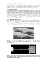
8.7.2 Application to Two-Dimensional Hypersonic Blunt Body Flow
The two-dimensional augmented Burnett code was employed to compute the hypersonic flow over a
cylindrical leading edge with a nose radius of 0.02 m in the continuum–transition regime. The grid sys-
tem (50 ϫ 82 mesh) used in the computations is shown in Figure 8.9. The results were compared with
those of Zhong (1991).
The flow conditions for this case are as follows:
M

∞
ϭ 10, Kn
∞
ϭ 0.1, Re
∞
ϭ 167.9,
P
∞
ϭ 2.3881 N/m
2
, T
∞
ϭ 208.4 K, T
w
ϭ 1000.0 K
The viscosity is calculated by Sutherland’s law,
µ
ϭ c
1
T
1.5
/(T ϩ c
2
). The coefficients c
1
and c
2
for air are
1.458 ϫ 10
Ϫ6

kg/(sec m K
1/2
) and 110.4K, respectively. Other constants used in this computation for air
are
γ
ϭ 1.4, Pr ϭ 0.72 and R ϭ 287.04 m
2
/(sec
2
K).
The comparisons of density, velocity, and temperature distributions along the stagnation streamline are
shown in Figures 8.10, 8.11, and 8.12 respectively. The results agree well with those of Zhong (1991) for
both the Navier–Stokes and the augmented Burnett computations. Because the flow is in the continuum–
transition regime (Kn ϭ 0.1), the Navier–Stokes equations become inaccurate, and the differences between
the Navier–Stokes and the augmented Burnett solutions are obvious. In particular, the difference between the
Navier–Stokes and Burnett solutions for the temperature distribution is significant across the shock.
Te mperature and Mach number contours of the Navier–Stokes solutions and the augmented Burnett
solutions are compared in Figures 8.13 and 8.14 respectively. The shock structure of the augmented
Burnett solutions agrees well with that of Zhong (1991). The shock layer of the augmented Burnett solutions
is thicker, and the shock location starts upstream of that of the Navier–Stokes solutions. However, because
the local Knudsen number decreases and the flow tends toward equilibrium as it approaches the wall surface,
the differences between the Navier–Stokes and augmented Burnett solutions become negligible near the
8-16 MEMS: Introduction and Fundamentals
0.5
0.4
0.3
0.2
0.1
0.0
1 2 3 4 5 6 7 8 91011

M
Navier−Stokes
Navier−Stokes
Woods
Simplified Woods
BGK−Burnett
Reciprocal density thickness
FIGURE 8.8 Plot showing the variation of reciprocal density thickness with Mach number, obtained with the
Navier–Stokes, Woods and Simplified Woods [Reese et al., 1995], and BGK–Burnett equations for a monatomic gas
(argon). Experimental data were obtained from Alsmeyer (1976). (Reprinted with permission from Alsmeyer, H.
(1976) “Density Profiles in Argon and Nitrogen Shock Waves Measured by the Absorption of an Electron Beam,”
J. Fluid Mech. 74, pp. 497–513.)
© 2006 by Taylor & Francis Group, LLC
wall, especially near the stagnation point. Thus, the Maxwell–Smoluchowski slip boundary conditions can be
applied for both the Navier–Stokes and the augmented Burnett calculations for the hypersonic blunt body.
8.7.3 Application to Axisymmetric Hypersonic Blunt Body Flow
The results of the axisymmetric augmented Burnett computations are compared with the DSMC results
obtained by Vogenitz and Takara (1971) for the axisymmetric hemispherical nose. The computed results
are also compared with Zhong and Furumoto’s (1995) axisymmetric augmented Burnett solutions. The
flow conditions for this case are
M
∞
ϭ 10, Kn
∞
ϭ 0.1
ϭ 1.0, ϭ 0.029
T
0
is the stagnation temperature. The gas is assumed to be a monatomic gas with a hard-sphere model.
The viscosity coefficient is calculated by the power law

µ
ϭ
µ
r
(T/T
r
)
0.5
. The reference viscosity
µ
r
and the
reference temperature T
r
used in this case are 2.2695 ϫ 10
Ϫ5
kg/(sec m) and 300 K, respectively. Other
constants used in this computation are
γ
ϭ 1.67 and Pr ϭ 0.67.
T
w
ᎏ
T
0
T
w
ᎏ
T
∞

Burnett Simulations of Flows in Microdevices 8-17
FIGURE 8.9 Two-dimensional computational grid (50 ϫ 82 mesh) around a blunt body, r
n
ϭ 0.02 m.
© 2006 by Taylor & Francis Group, LLC
The comparisons of density and temperature distributions along the stagnation streamline among the
current axisymmetric augmented Burnett solutions, the axisymmetric augmented Burnett solutions of
Zhong and Furumoto, and the DSMC results are shown in Figures 8.15 and 8.16,respectively. The corre-
sponding Navier–Stokes solutions are also compared in these figures. The axisymmetric augmented
Burnett solutions agree well with Zhong and Furumoto’s axisymmetric augmented Burnett solutions in
both density and temperature. The density distributions for both the Navier–Stokes and augmented
8-18 MEMS: Introduction and Fundamentals
0
5
10
15
25
20
Nondimensional density (␳/␳
∞
)
−0.25
x/r
n
Navier−Stokes
Navier−Stokes (Zhong)
Augmented Burnett
Augmented Burnett (Zhong)
−1
0

−0.75 −0.5
FIGURE 8.10 Density distributions along stagnation streamline for blunt body flow: air, M
∞
ϭ 10, and Kn
∞
ϭ 0.1.
0
2500
3000
2000
1500
1000
500
Velocity (m/sec)
Navier−Stokes
Navier−Stokes (Zhong)
Augmented Burnett
Augmented Burnett (Zhong)
x/r
n
−1
0
−0.75 −0.5 −0.25
FIGURE 8.11 Velocity distributions along stagnation streamline for blunt body flow: air, M
∞
ϭ 10, and Kn
∞
ϭ 0.1.
© 2006 by Taylor & Francis Group, LLC
Burnett equations show little differences from the DSMC results. The temperature distributions, however,

show that the DSMC method predicts a thicker shock than the augmented Burnett equations. The max-
imum temperature of the DSMC results is slightly higher than those of the augmented Burnett solutions.
However, the augmented Burnett solutions show much closer agreement with the DSMC results than the
Navier–Stokes solutions.
Burnett Simulations of Flows in Microdevices 8-19
0
5000
4000
3000
2000
1000
Temperature (␤K)
x/r
n
−1
0
−0.75 −0.5 −0.25
Navier−Stokes
Navier−Stokes (Zhong)
Augmented Burnett
Augmented Burnett (Zhong)
FIGURE 8.12 Temperature distributions along stagnation streamline for blunt body flow: air, M
∞
ϭ 10, and
Kn
∞
ϭ 0.1.
Augmented Burnett
Navier−Stokes
FIGURE 8.13 Comparison of temperature contours for blunt body flow: air, M

∞
ϭ 10, and Kn
∞
ϭ 0.1.
© 2006 by Taylor & Francis Group, LLC
Overall, the axisymmetric augmented Burnett solutions presented here agree well with Zhong and
Furumoto’s (1995) axisymmetric augmented Burnett solutions and describe the shock structure closer to
the DSMC results than the Navier–Stokes solutions.
As another application to the hypersonic blunt body, the augmented Burnett equations are applied to
compute the hypersonic flow field at re-entry condition encountered by the nose region of the space shuttle.
8-20 MEMS: Introduction and Fundamentals
Navier−Stokes
Augmented Burnett
FIGURE 8.14 Comparison of Mach number contours for blunt body flow: air, M
∞
ϭ 10, and Kn
∞
ϭ 0.1.
0
Navier−Stokes
50
40
30
20
10
−0.7 −0.6 −0.5 −0.4 −0.3 −0.2 −0.1
Augmented Burnett
Augmented Burnett (Zhong and Furumoto)
DSMC (Vogenitz and Takara)
x/r

n
␳/␳
∞
FIGURE 8.15 Density distributions along stagnation streamline for a hemispherical nose: hard-sphere gas, M
∞
ϭ 10
and Kn
∞
ϭ 0.1.
© 2006 by Taylor & Francis Group, LLC
The computations are compared with the DSMC results of Moss and Bird (1984). The DSMC method
accounts for the translational, rotational, vibrational, and chemical nonequilibrium effects.
An equivalent axisymmetric body concept [Moss and Bird, 1984] is applied to model the windward cen-
terline of the space shuttle at a given angle of attack. Ahyperboloid with nose radius of 1.362m and
asymptotic half angle of 42.5° is employed as the equivalent axisymmetric body to simulate the nose of
the shuttle. Figure 8.17 shows the side view of the grid (61 ϫ 100 mesh) around the hyperboloid. The
freestream conditions at an altitude of 104.93 km as given in Moss and Bird (1984) are
M
∞
ϭ 25.3, Kn
∞
ϭ 0.227, Re
∞
ϭ 163.8,
ρ
∞
ϭ 2.475 ϫ 10
Ϫ7
kg/m
3

, T
∞
ϭ 223 K, T
w
ϭ 560 K
The viscosity is calculated by the power law. The reference viscosity
µ
r
and the reference temperature T
r
are taken as 1.47 ϫ 10
Ϫ5
kg/(sec m) and 223 K, respectively.
Figures 8.18 and 8.19 show comparisons of the density and temperature distributions along the stagna-
tion streamline between the Navier–Stokes solutions, the augmented Burnett solutions, and the DSMC
results. The differences between the augmented Burnett solutions and the DSMC results are significant in
both density and temperature distributions. In Figure 8.18, the density distribution of the DSMC results is
lower and smoother than that of the augmented Burnett solutions. In Figure 8.19, the DSMC method pre-
dicts about 30% thicker shock layer and 9% lower maximum temperature than the augmented Burnett
equations. The DSMC results can be considered to be more accurate than the augmented Burnett solutions
as the DSMC method accounts for all the effects of translational, rotational, vibrational, and chemical non-
equilibrium, while the augmented Burnett equations do not. However, the augmented Burnett solutions
agree much better with the DSMC results than the Navier–Stokes computations. The difference between
the Navier–Stokes solutions and the augmented Burnett solutions in temperature distributions is very sig-
nificant. The shock layer of the augmented Burnett solutions is almost two times thicker than the
Navier–Stokes solutions. The augmented Burnett solutions predict about 11% less maximum temperature
than the Navier–Stokes solutions.
Burnett Simulations of Flows in Microdevices 8-21
0
5

10
15
25
20
30
35
Navier−Stokes
Augmented Burnett
(Zhong and Furumoto)
Augmented Burnett
DSMC (Vogenitz and Takara)
−1
0
−0.75 −0.5 −0.25
x/r
n
T/ T
∞
FIGURE 8.16 Temperature distribution along stagnation streamline for a hemispherical nose: hard-sphere gas,
M
∞
ϭ 10 and Kn
∞
ϭ 0.1.
© 2006 by Taylor & Francis Group, LLC
8.7.4 Application to NACA 0012 Airfoil
The Navier–Stokes equations are applied to compute the rarefied subsonic flow over a NACA 0012 airfoil
with chord length of 0.04 m. The grid system in the physical domain is shown in Figure 8.20. The flow
conditions are
M

∞
ϭ 0.8, Re
∞
ϭ 73,
ρ
∞
ϭ 1.116 ϫ 10
Ϫ4
kg/m
3
, T
∞
ϭ 257 K, and Kn
∞
ϭ 0.014
Various constants used in the calculation for air are
γ
ϭ 1.4, Pr ϭ 0.72, and R ϭ 287.04 m
2
/(sec
2
K).
Figure 8.21 shows the density contours of the Navier–Stokes solution with the first-order Maxwell–
Smoluchowski slip-boundary conditions. These contours using the continuum approach agree well with
those of Sun et al. (2000) using the information preservation (IP) particle method. At these Mach and
Knudsen numbers, the contours from the DSMC calculations are not smooth due to the statistical scatter.
The comparison of pressure distribution along the surface between our Navier–Stokes solution with a slip-
boundary condition and the DSMC calculation [Sun et al., 2000] is shown in Figure 8.22; the agreement
between the solutions is good. Figure 8.23 compares the surface slip velocity from the DSMC, IP, and
Navier–Stokes methods as calculated by Sun et al. and by our Navier–Stokes calculation. The slip velocity

8-22 MEMS: Introduction and Fundamentals
␣ = 0°
r
n
FIGURE 8.17 Side view of the grid (61 ϫ 100 mesh) around a hyperboloid nose of radius r
n
ϭ 1.362 m.
© 2006 by Taylor & Francis Group, LLC
distribution from our Navier–Stokes calculation shows good agreement with that obtained from the
DSMC and IP methods except near the trailing edge. However, our Navier–Stokes results disagree consid-
erably with those reported in Sun et al. (2000). This calculation again demonstrates that Navier–Stokes
equations with slip-boundary conditions can provide accurate flow simulation 0.001 Ͻ Kn Ͻ 0.1.
8.7.5 Subsonic Flow in a Microchannel
The augmented Burnett equations are employed for computation of subsonic flow in a microchannel
with a ratio of channel length to height of 20 (L/H ϭ 20). For the wall boundary conditions, Beskok’s and
Burnett Simulations of Flows in Microdevices 8-23
0
DSMC (Moss and Bird)
Augmented Burnett
Navier−Stokes
10
−4
10
−5
10
−6
10
−7
−1.2 −1 −0.8 −0.6 −0.4 −0.2
x (m)

␳ (kg /m
3
)
FIGURE 8.18 Density distributions along stagnation streamline for a hyperboloid nose: air, M
∞
ϭ 25.3 and
Kn
∞
ϭ 0.227.
0
0
15000
20000
10000
5000
DSMC (Moss and Bird)
Augmented Burnett
Navier−Stokes
−1.4
−1.2
−0.8 −0.6 −0.4 −0.2−1
x (m)
T (°K)
FIGURE 8.19 Temperature distributions along stagnation streamline for a hyperboloid nose: air, M
∞
ϭ 25.3 and
Kn
∞
ϭ 0.227.
© 2006 by Taylor & Francis Group, LLC

8-24 MEMS: Introduction and Fundamentals
6
4
2
0
−2
−4
−6
−6 −4 −2 0 2 4 6
x/c
y/c
FIGURE 8.20 Grid (101 ϫ 91 mesh) around a NACA 0012 airfoil, c ϭ 0.04 m.
−0.1
0.1
0.2
0.3
0.4
0.5
0.6
0.7
0.8
0.9
0
1
1.1
−0.1
0.1
0.2
0.3
0.4

0.5
0.6
0.7
0.8
0.9
0
1
1.1
0 0.1 0.2 0.3 0.4 0.5 0.6 0.7 0.8 0.9 1 1.1
−0.3 −0.2 −0.1
0 0.1 0.2 0.3 0.4 0.5 0.6 0.7 0.8 0.9 1 1.1
−0.3−0.2−0.1
y/c
x/c
1.28
1.24
1.20
1.16
1.04
0.96
0.92
0.84
0.88
1.00
1.08
1.04
1.12
0.96
1.00
FIGURE 8.21 Density contours for NACA 0012 airfoil: air, M

∞
ϭ 0.8 and Kn
∞
ϭ 0.014; Navier–Stokes solution with
first-order slip boundary condition.
© 2006 by Taylor & Francis Group, LLC
Burnett Simulations of Flows in Microdevices 8-25
x/c
0 10.25 0.5 0.75
0 10.25 0.5 0.75
0
1
2
−1
−0.5
1.5
0.5
0
1
2
−1
−0.5
1.5
0.5
DSMC (Sun et al.)
Present N−S
(P − P
∝
)/(0.5␳
∝

V
2
∝
)
FIGURE 8.22 Pressure distributions along NACA 0012 airfoil surface: air, M
∞
ϭ 0.8 and Kn
∞
ϭ 0.014.
0
0
0.25
0.25
0.5
0.5
0.75
0.75
1
1
x/c
0
0
0.05 0.0
5
0.1 0.1
0.15 0.1
5
0.2
0.2
0.25 0.2

5
Present N−S
N−S (Sun et al.)
IP (Sun et al.)
DSMC (Sun et al.)
U
s
/ U
∝
FIGURE 8.23 Slip velocity distributions along NACA 0012 airfoil surface: air, M
∞
ϭ 0.8 and Kn
∞
ϭ 0.014.
© 2006 by Taylor & Francis Group, LLC
Langmuir’s boundary conditions are employed and compared. The augmented Burnett solutions are also
compared with the Navier–Stokes solutions. Flow conditions at the entrance and exit of the channel are
Kn
in
ϭ 0.088, Kn
out
ϭ 0.2 and P
in
/P
out
ϭ 2.28.
Figure 8.24 compares the velocity profiles at various streamwise locations. Both Navier–Stokes and aug-
mented Burnett equations using either Beskok’s or Langmuir’s boundary conditions show almost identical
velocity profiles. These velocity profiles agree well with the velocity profiles from the micro-flow calculation
by Beskok and Karniadakis (1999). Nondimensional mass flow rates along the microchannel are shown in

Figure 8.25. All the mass flow rates from both equations and both slip-boundary conditions are about 0.76
and almost constant along the channel, as should be the case. This mass flow rate is 13% higher than that
8-26 MEMS: Introduction and Fundamentals
0
0.5
1
y/y
max
0
0.5
1
y/y
max
0
0.5
1
0.50 1 21.5
Kn = 0.12
x/L = 0.5
Kn = 0.15
x/L = 0.8
x/L = 0.2
Kn = 0.09
Navier−Stokes, Beskok's
BC
Aug. Burnett, Beskok's BC
Navier−Stokes,
Langmuir's BC
Aug. Burnett, Langmuir's
BC

U/U
1
y/y
max
FIGURE 8.24 Comparison of velocity profiles at various streamwise locations: Kn
in
ϭ 0.088, Kn
out
ϭ 0.2 and
P
in
/P
out
ϭ 2.28.
Mass flow rate
0.0
5.0 10.0
15.0
20.0
x/y
max
1
0.8
0.6
0.4
0.2
0
Navier−Stokes, Beskok's BC
Aug. Burnett, Beskok's BC
Navier−Stokes, Langmuir's BC

Aug. Burnett, Langmuir's BC
FIGURE 8.25 Comparison of mass flow rates along the microchannel: Kn
in
ϭ 0.088, Kn
out
ϭ 0.2 and P
in
/P
out
ϭ 2.28.
© 2006 by Taylor & Francis Group, LLC
predicted with a no-slip-boundary condition, which is 0.667. Figure 8.26 shows comparison of pressure
distribution along the centerline. Both the Navier–Stokes and the augmented Burnett equations show a
nonconstant pressure gradient along the channel. The solutions using Beskok’s slip-boundary condition
show less change in pressure gradient than those from the Langmuir’s boundary condition. Figure 8.27
compares the streamwise velocity distributions along the centerline. The streamwise velocity distributions
are almost identical except near the exit. Figure 8.28 compares the slip velocity distributions along the wall.
The slip velocity profiles obtained from both Navier–Stokes and augmented Burnett equations are
identical when the same wall-boundary conditions are employed. However, the Beskok’s slip-boundary
condition and Langmuir’s slip-boundary condition show a large difference. The Beskok’s slip-boundary
Burnett Simulations of Flows in Microdevices 8-27
1
1.2
1.4
1.6
1.8
2.2
2.4
0.0 5.0 10.0 15.0 20.0
x/y

max
2
P/P
out
Navier−Stokes, Beskok's BC
Aug. Burnett, Beskok's BC
Navier−Stokes, Langmuir's BC
Aug. Burnett, Langmuir's BC
FIGURE 8.26 Comparison of pressure distribution along the centerline: Kn
in
ϭ 0.088, Kn
out
ϭ 0.2 and
P
in
/P
out
ϭ 2.28.
1
1.2
1.4
1.6
1.8
2.2
2.4
0.0
5.0 10.0
15.0
20.0
x/y

max
2
U/ U
1
Navier−Stokes, Beskok's BC
Aug. Burnett, Beskok's BC
Navier−Stokes, Langmuir's BC
Aug. Burnett, Langmuir's BC
FIGURE 8.27 Comparison of streamwise velocity distributions along the centerline: Kn
in
ϭ 0.088, Kn
out
ϭ 0.2 and
P
in
/P
out
ϭ 2.28.
0
0.2
0.4
0.6
0.8
1
0.0 5.0
10.0
15.0
20.0
x/y
max

U/U
1
Navier−Stokes, Beskok's BC
Aug. Burnett, Beskok's BC
Navier−Stokes, Langmuir's BC
Aug. Burnett, Langmuir's BC
FIGURE 8.28 Comparison of slip velocity distributions along the wall: Kn
in
ϭ 0.088, Kn
out
ϭ 0.2 and
P
in
/P
out
ϭ 2.28.
© 2006 by Taylor & Francis Group, LLC
condition predicts lower slip velocity near the entrance and higher slip velocity near the exit. As the figures
show, there is very little difference between the Navier–Stokes solutions and the augmented Burnett solu-
tions at the entrance, but as the local Knudsen number increases toward the exit of the channel, the dif-
ference between the Navier–Stokes solutions and the augmented Burnett solutions increases as expected.
8.7.6 Supersonic Flow in a Microchannel
The Navier–Stokes equations and the augmented Burnett equations are applied to compute the super-
sonic flow in a microchannel. The geometry and grid of the microchannel are shown in Figure 8.29. As
the flow enters the channel, the tangential velocity component to the wall is retained, while the velocity
component normal to the wall is neglected at wall boundaries in the region 0 Յ x Յ 1 µm. The first-order
8-28 MEMS: Introduction and Fundamentals
y/y
max
0.0

0.5
1.0
0.0 1.0 2.0 3.0 4.0 5.0
x/y
max
FIGURE 8.29
Microchannel geometry and grid.
y/y
max
1.0
0.5
0.0
0.0
1.0
2.0
3.0 4.0 5.0
y/y
max
1.0
0.5
0.0
0.0
1.0
2.0
3.0 4.0 5.0
x/y
max
(a)
(b)
x/y

max
(c)
y/y
max
1.0
0.5
0.0
Navier−
Stokes
Navier−
Stokes
Augmented
Burnett
Augmented
Burnett
0.0 1.0 2.0 3.0 4.0 5.0
x/y
max
Navier−
Stokes
Augmented
Burnett
FIGURE 8.30 Comparisons of contours between Navier–Stokes and augmented Burnett equations: helium, M
∞
ϭ 5
and Kn
∞
ϭ 0.7.
© 2006 by Taylor & Francis Group, LLC
Maxwell–Smoluchowski slip-boundary conditions are employed at the rest of the wall boundaries. The

channel height and length are 2.4 and 12 µm, respectively. The flow conditions at the entrance for the
helium flow are
M
∞
ϭ 5.0, P
∞
ϭ 1.01 ϫ 10
6
dyne/cm
2
,
Kn
∞
ϭ 0.07, T
∞
ϭ 298 K
Burnett Simulations of Flows in Microdevices 8-29
0.0 1.0 2.0 3.0 4.0 5.0
x/y
max
0.0 1.0 2.0 3.0 4.0 5.0
x/y
max
0.0 1.0 2.0 3.0 4.0 5.0
x/y
max
0
1500
1000
500

Mach number Temperature (K) Density (g/cm
3
)
6.0E−04
5.0E−04
4.0E−04
3.0E−04
2.0E−04
1.0E−04
0.0E+00
0.0 1.0 2.0 3.0 4.0 5.0
x/y
max
Navier−Stokes
Augmented Burnett
DSMC (Oh et al.)
1.5E+07
1.0E+07
5.0E+06
0.0E+00
Pressure (dyne/cm
2
)
5.0
4.0
3.0
2.0
1.0
0.0
FIGURE 8.31 Comparisons of density, temperature, pressure, and Mach number profiles along the centerline of the

channel: helium, M
∞
ϭ 5 and Kn
∞
ϭ 0.7.
© 2006 by Taylor & Francis Group, LLC
Figure 8.30 compares the pressure, Mach number, and temperature contours obtained from the
Navier–Stokes and augmented Burnett equations. Solutions from the Navier–Stokes and augmented
Burnett equations do not show significant differences. These flow property contours also agree well with
the DSMC solutions obtained by Oh et al. (1997). Figure 8.31 compares the density, temperature, pres-
sure, and Mach number profiles along the centerline of the channel using the Navier–Stokes, augmented
Burnett, and DSMC formulations [Oh et al., 1997]. The profiles generally agree well with the DSMC
results. The temperature and Mach number profiles especially show very close agreement with the DSMC
8-30 MEMS: Introduction and Fundamentals
0.0 1.0 2.0 3.0 4.0 5.0
0.0 1.0 2.0 3.0 4.0 5.0
0.0 1.0 2.0 3.0 4.0 5.0
0
Navier−Stokes
Augmented Burnett
1500
1000
500
Mach number Temperature (K)
DSMC (Oh et al.)
0.0 1.0 2.0 3.0 4.0 5.0
x/y
max
x/y
max

x/y
max
x/y
max
2.0E−03
1.7E−03
1.5E−03
1.2E−03
1.0E−03
7.5E−04
5.0E−04
2.5E−04
0.0E+00
Density (g/cm
3
)Pressure (dyne/cm
2
)
1.5E+07
1.0E+07
5.0E+06
0.0E+00
5.0
4.0
3.0
2.0
0.0
1.0
FIGURE 8.32 Comparisons of density, temperature, pressure, and Mach number profiles along the wall of the chan-
nel: helium, M

∞
ϭ 5 and Kn
∞
ϭ 0.7.
© 2006 by Taylor & Francis Group, LLC
results. The augmented Burnett solutions are closer to the DSMC solutions than the Navier–Stokes solu-
tions in the temperature and Mach number profiles. Figure 8.32 compares the density, temperature, pres-
sure, and Mach number profiles along the channel wall using the Navier–Stokes, augmented Burnett, and
DSMC formulations. Both the Navier–Stokes and augmented Burnett solutions show some difference
with the DSMC solutions. Figures 8.33 and 8.34 compare the temperature and velocity profiles across the
channel at various streamwise locations using the Navier–Stokes, augmented Burnett, and DSMC for-
mulations respectively. The profiles obtained from the augmented Burnett solutions are closer to the
DSMC results than the Navier–Stokes solutions.
Unfortunately, experimental data are not available to assess the accuracy of the Navier–Stokes, Burnett,
and DSMC models for computing the microchannel flows. A substantial amount of both experimental
Burnett Simulations of Flows in Microdevices 8-31
0 500 1000
1500
Temperature (K)
y/y
max
1
0.9
0.8
0.7
0.6
0.5
0.4
0.3
0.2

0.1
0
0 500 1000
1500
Temperature (K)
y/y
max
1
0.9
0.8
0.7
0.6
0.5
0.4
0.3
0.2
0.1
0
0
0
500 1000
1500
Temperature (K)
y/ y
max
1
0.9
0.8
0.7
0.6

0.5
0.4
0.3
0.2
0.1
0 500 1000
1500
Temperature (K)
0 500 1000 15000
y/y
max
1
0.9
0.8
0.7
0.6
0.5
0.4
0.3
0.2
0.1
0
500 1000 1500
x = 0.8
y/y
max
1
0.9
0.8
0.7

0.6
0.5
0.4
0.3
0.2
0.1
0
y/y
max
x = 1.6
x = 3.2x = 2.4
x = 4.0
x = 4.8
Temperature (K)Temperature (K)
1
0.9
0.8
0.7
0.6
0.5
0.4
0.3
0.2
0.1
0
Navier−Stokes
Augmented Burnett
DSMC (Oh et al.)
FIGURE 8.33 Comparisons of temperature profiles across the channel at various streamwise locations: helium,
M

∞
ϭ 5 and Kn
∞
ϭ 0.7.
© 2006 by Taylor & Francis Group, LLC
and computational simulation work is needed to determine the applicability and accuracy of various
fluid models for computing high Knudsen number flow in microchannels.
8.8 Conclusions
For computing flows in the continuum–transition regime, higher order fluid dynamics models beyond
Navier–Stokes are needed. These models are known as extended, or generalized, hydrodynamics models
in the literature. Some of these models are the Burnett equations; 13-moment Grad’s equations; Gaussian
closure or Levermore moment equations; and Eu’s equations. An alternative to generalized hydrodynamic
8-32 MEMS: Introduction and Fundamentals
0 250000 500000
u (cm/sec)
y/y
max
1
0.9
0.8
0.7
0.6
0.5
0.4
0.3
0.2
0.1
0
0 250000 500000
u (cm/sec)

y/y
max
1
0.9
0.8
0.7
0.6
0.5
0.4
0.3
0.2
0.1
0
0 250000 500000
u (cm/sec)
y/y
max
1
0.9
0.8
0.7
0.6
0.5
0.4
0.3
0.2
0.1
0
0 250000 500000
u (cm/sec)

y/y
max
1
0.9
0.8
0.7
0.6
0.5
0.4
0.3
0.2
0.1
0
0 250000 500000
1
0.9
0.8
0.7
0.6
0.5
0.4
0.3
0.2
0.1
0
0 250000 500000
u (cm/sec)
0
250000 500000
x

=
1.6
x
=
3.2
x
=
2.4
x
=
4.0 x
=
4.8
x = 0.8
y/y
max
1
0.9
0.8
0.7
0.6
0.5
0.4
0.3
0.2
0.1
0
y/y
max
Navier−Stokes

Augmented
Burnett
DSMC (Oh et al.)
u (cm/sec)
1
0.9
0.8
0.7
0.6
0.5
0.4
0.3
0.2
0.1
0
FIGURE 8.34 Comparisons of velocity profiles across the channel at various streamwise locations: helium, M
∞
ϭ 5
and Kn
∞
ϭ 0.7.
© 2006 by Taylor & Francis Group, LLC
models is the hybrid approach, which combines a Euler or Navier–Stokes solver with the DSMC method.
Most of the generalized hydrodynamic models proposed to date suffer from the following drawbacks:
they do not capture the physics properly or they are too computationally intensive, or both. In this chap-
ter, the history of a set of extended hydrodynamics equations based on the Chapman–Enskog expansion
of Boltzmann equations to O(Kn
2
) known as the Burnett equations has been reviewed. The various sets
known in the literature as conventional, augmented, and BGK–Burnett equations have been considered

and critically examined. Computations for hypersonic flows and microscale flows show that both the aug-
mented and BGK–Burnett equations can be effectively applied to accurately compute flows in the con-
tinuum–transition regime. However, a great deal of additional work is needed, both experimentally and
computationally, to assess the range of applicability and accuracy of Navier–Stokes, Burnett, and DSMC
approximations for simulating the flows in transition regime.
References
Alsmeyer, H. (1976) “Density Profiles in Argon and Nitrogen Shock Waves Measured by the Absorption
of an Electron Beam,” J. Fluid Mech. 74, pp. 497–513.
Arkilic, E.B., Schmidt, M.A., and Breuer, K.S. (1997) “Gaseous Flow in Long Microchannel,” J. MEMS 6,
pp. 167–78.
Balakrishnan, R. (1999) Entropy Consistent Formulation and Numerical Simulation of the BGK–Burnett
Equations for Hypersonic Flows in the Continuum–Transition Regime, Ph.D. thesis, Wichita State
University.
Balakrishnan, R., and Agarwal, R.K. (1996) “Entropy Consistent Formulation and Numerical Simula-
tion of the BGK–Burnett Equations for Hypersonic Flows in the Continuum–Transition
Regime,” in Proc. of the 15th Int. Conf. on Numerical Methods in Fluid Dynamics, Lecture Note in
Physics, Springer–Verlag, New York, pp. 480–85.
Balakrishnan, R., and Agarwal, R.K. (1997) “Numerical Simulation of the BGK–Burnett for Hypersonic
Flows,” J. Thermophys. Heat Transf. 11, pp. 391–99.
Balakrishnan, R., and Agarwal, R.K. (1999) “A Comparative Study of Several Higher-Order Kinetic
Formulations Beyond Navier–Stokes for Computing the Shock Structure,” AIAA Paper 99-0224,
American Institute of Aeronautics and Astronomics, Reno, NV.
Balakrishnan, R., Agarwal, R.K., and Yun, K.Y. (1997) “Higher-Order Distribution Functions,
BGK–Burnett Equations, and Boltzmann’s H-Theorem,” AIAA Paper 97-2552, American Institute
of Aeronautics and Astronomics, Atlanta, GA.
Beskok, A., and Karniadakis, G. (1999) “A Model for Flows in Channels, Pipes, and Ducts at Micro and
Nano Scales,” Microscale Thermophys. Eng. 8, pp. 43–77.
Beskok, A., Karniadakis, G., and Trimmer, W. (1996) “Rarefaction and Compressibility Effects in Gas
Microflows,” J. Fluid Eng. 118, pp. 448–56.
Bhatnagar, P.L., Gross, E.P., and Krook, M. (1954) “A Model for Collision Process in Gas,” Phys. Rev. 94,

pp. 511–25.
Bird, G.A. (1994) Molecular Gas Dynamics and the Direct Simulation of Gas Flows, Oxford Science
Publications, New York.
Bobylev, A.V. (1982) “The Chapman–Enskog and Grad Methods for Solving the Boltzmann Equation,”
Sov. Phys. Doklady 27, pp. 29–31.
Boyd, I., Chen, G., and Candler, G. (1995) “Predicting Failure of the Continuum Fluid Equations in
Transitional Hypersonic Flows,” Phys. Fluids 7, pp. 210–19.
Brown, S. (1996) Approximate Riemann Solvers for Moment Models of Dilute Gases, Ph.D. thesis,
University of Michigan.
Burnett, D. (1935) “The Distribution of Velocities and Mean Motion in a Slight Non-Uniform Gas,” Proc.
London Math. Soc. 39, pp. 385–430.
Chapman, S., and Cowling, T.G. (1970) The Mathematical Theory of Non-Uniform Gases, Cambridge
University Press, New York.
Burnett Simulations of Flows in Microdevices 8-33
© 2006 by Taylor & Francis Group, LLC
Comeaux, K.A., Chapman, D.R., and MacCormack, R.W. (1995) “An Analysis of the Burnett Equations
Based in the Second Law of Thermodynamics,” AIAA Paper 95-0415, American Institute of
Aeronautics and Astronautics, Reno, NV.
Eu, B.C. (1992) Kinetic Theory and Irreversible Thermodynamics, John Wiley & Sons, New York.
Fiscko, K.A., and Chapman, D.R. (1988) “Comparison of Burnett, Super-Burnett and Monte Carlo
Solutions for Hypersonic Shock Structure,” in Proc. 16th Int. Symp. on Rarefied Gas Dynamics,
Pasadena, CA, July 1988, American Institute of Physics, pp. 374–95.
Gad-el-Hak, M. (1999) “The Fluid Mechanics of Microdevices,” J. Fluids Eng. 121, pp. 5–33.
Grad, H. (1949) “On the Kinetic Theory of Rarefied Gases,” Comm. Pure Appl. Math. 2, pp. 325–31.
Groth, C.P.T., Roe, P.L., Gombosi, T.I., and Brown, S.L. (1995) “On the Nonstationary Wave Structure of
35-Moment Closure for Rarefied Gas Dynamics,” AIAA Paper 95-2312, American Institute of
Aeronautics and Astronautics, San Diego, CA.
Harley, J.C., Huang, Y., Bau, H.H., and Zemel, J.N. (1995) “Gas Flow in Microchannels,” J. Fluid Mech.
284, pp. 257–74.
Holway, L.H. (1964) “Existence of Kinetic Theory Solutions to the Shock Structure Problem,” Phys. Fluids

7, pp. 911–13.
Ivanov, M.S., and Gimelshein, S.F. (1998) “Computational Hypersonic Rarefied Flows,” Annu. Rev. Fluid
Mech. 30, pp. 469–505.
Koppenwallner, G. (1987) “Low Reynolds Number Influence on the Aerodynamic Performance of
Hypersonic Lifting Vehicles,” Aerodyn. Hypersonic Lifting Vehicles (AGARD, CP-428) 11, pp. 1–14.
Lee, C.J. (1994) “Unique Determination of Solutions to the Burnett Equations,” AIAA J. 32, pp. 985–90.
Levermore, C.D. (1996) “Moment Closure Hierarchies for Kinetic Theory,” J. Stat. Phys. 83, pp. 1021–65.
Levermore, C.D., and Morokoff, W.J. (1998) “The Gaussian Moment Closure for Gas Dynamics,” SIAM J.
Appl. Math. 59, pp. 72–96.
Liu, J.Q., Tai, Y.C., Pong, K.C., and Ho, C.M. (1993) “Micromachined Channel/Pressure Sensor Systems
for Micro Flow Studies,” in Proc. of the 7th Int. Conf. on Solid-State Sensors and Actuators—
Transducers ’93, Yokohama, Japan, 7–10 June, pp. 995–98.
Moss, J.N., and Bird, G.A. (1984) “Direct Simulation of Transitional Flow for Hypersonic Reentry
Conditions,” AIAA Paper 84-0223, American Institute of Aeronautics and Astronautics, Reno, NV.
Myong, R. (1999) “A New Hydrodynamic Approach to Computational Hypersonic Rarefied Gas
Dynamics,”AIAA Paper 99-3578, American Institute of Aeronautics and Astronautics, Norfolk,VA.
Nance, R.P., Hash, D.B., and Hassan, H.A. (1998) “Role of Boundary Conditions in Monte Carlo
Simulation of Microelectromechanical Systems,” J. Spacecraft Rockets 12, pp. 447–49.
Oh, C.K., Oran, E.S., and Sinkovits, R.S. (1997) “Computations of High-Speed, High Knudsen Number
Microchannel Flows,” J. Thermophys. Heat Transf. 11, pp. 497–505.
Oran, E.S., Oh, C.K., and Cybyk, B.Z. (1998) “Direct Simulation Monte Carlo: Recent Advances and
Application,” Annu. Rev. Fluid Mech. 30, pp. 403–41.
Pong, K.C., Ho, C.M., Liu, J.Q., and Tai, Y.C. (1994) “Non-Linear Pressure Distribution in Uniform
Microchannels,” ASME FED 197, pp. 51–56.
Reese, J.M., Woods, L.C., Thivet, F.J.P., and Candel, S.M. (1995) “A Second-Order Description of Shock
Structure,” J. Comput. Phys. 117, pp. 240–50.
Roveda, R., Goldstein, D.B., and Varghese, P.L. (1998) “Hybrid Euler/Particle Approach for
Continuum/Rarefied Flows,” J. Spacecraft Rockets 35, pp. 258–65.
Smoluchowski, von M. (1898) “Veder Warmeleitung in Verdumteu Gasen,” Ann. Phys. Chem. 64,
pp. 101–30.

Steger, J.L., and Warming, R.F. (1981) “Flux Vector Splitting of the Inviscid Gas Dynamics Equations with
Application to Finite-Difference Methods,” J. Comput. Phys. 40, pp. 263–93.
Sun, Q., Boyd, I.D., and Fan, J. (2000) “Development of Particle Methods for Computing MEMS Gas
Flows,” J. MEMS 2, pp. 563–69.
Vogenitz, F.W., and Takara, G.Y. (1971) “Monte Carlo Study of Blunt Body Hypersonic Viscous Shock
Layers,” Rarefied Gas Dynamics 2, pp. 911–18.
8-34 MEMS: Introduction and Fundamentals
© 2006 by Taylor & Francis Group, LLC
Weiss, W. (1996) “Comments on Existence of Kinetic Theory Solutions to the Shock Structure Problem,”
Phys. Fluids 8, pp. 1689–90.
Welder, W.T., Chapman, D.R., and MacCormack, R.W. (1993) “Evaluation of Various Forms of the
Burnett Equations,” AIAA Paper 93-3094, American Institute of Aeronautics and Astronautics,
Orlando, FL.
Yun, K.Y., and Agarwal, R.K. (2000) “Numerical Simulation of 3-D Augmented Burnett Equations for
Hypersonic Flow in Continuum–Transition Regime,” AIAA Paper 2000-0339, American Institute
of Aeronautics and Astronautics, Reno, NV.
Yun, K.Y.,Agarwal, R.K., and Balakrishnan, R. (1998a) Three-Dimensional Augmented and BGK–Burnett
Equations, unpublished report, Wichita State University.
Yun, K.Y., Agarwal, R.K., and Balakrishnan, R. (1998b) “Augmented Burnett and Bhatnagar–
Gross–Krook–Burnett for Hypersonic Flow,” J. Thermophys. Heat Transf. 12, pp. 328–35.
Zhong, X. (1991) Development and Computation of Continuum Higher Order Constitutive Relations for
High-Altitude Hypersonic Flow, Ph.D. thesis, Stanford University.
Zhong, X., and Furumoto, G. (1995) “Augmented Burnett Equation Solutions over Axisymmetric Blunt
Bodies in Hypersonic Flow,” J. Spacecraft Rockets 32, pp. 588–95.
Burnett Simulations of Flows in Microdevices 8-35
© 2006 by Taylor & Francis Group, LLC