The MEMS Handbook Introduction & Fundamentals (2nd Ed) - M. Gad el Hak Part 9 ppsx

of the fluid outside of the EDL as a three-dimensional, unsteady flow of a viscous fluid of zero net charge
that is bounded by the following slip velocity condition:
u
slip
ϭ E
slip
(10.50)
where the subscript slip indicates a quantity evaluated at the slip surface at the top of the EDL (in prac-
tice, a few Debye lengths from the wall). The velocity along this slip surface is, for thin EDLs, similar to
the electric field. This equation and the condition of similarity also hold for inlets and outlets of the flow
domain that have zero imposed pressure-gradients.
The complete velocity field of the flow bounded by the slip surface (and inlets and outlets) can be shown
to be similar to the electric field [Santiago, 2001]. We nondimensionalize the Navier–Stokes equations by
a characteristic velocity and length scale U
s
and L
s
, respectively. The pressure p is nondimensionalized by the
viscous pressure
µ
U
s
/L
s
. The Reynolds and Strouhal numbers are Re ϭ
ρ
L
s
U
s
/

µ
and St ϭ L
s
/
τ
U
s
, respec-
tively, where τ is the characteristic time scale of a forcing function. The equation of motion is
ReSt ϩ Re(uЈ и ∇uЈ) ϭ Ϫ∇pЈ ϩ ∇
2
uЈ (10.51)
Note that the right-most term in Equation (10.51) can be expanded using a well-known vector identity
∇
2
uЈ ϭ ∇(∇ и uЈ) Ϫ ∇ ϫ ∇ ϫ uЈ. (10.52)
We can now propose a solution to Equation (10.52) that is proportional to the electric field and of the form
uЈ ϭ E (10.53)
where c
o
is a proportionality constant, and E is the electric field driving the fluid. Since we have assumed
that the EDL is thin, the electric field at the slip surface can be approximated by the electric field at the
wall. The electric field bounded by the slip surface satisfies Faraday’s and Gauss’ laws,
∇ и E ϭ ∇ ϫ E ϭ 0 (10.54)
Substituting Equation (10.53) and Equation (10.54) into Equation (10.51) yields
ReSt ϩ Re(uЈ и ∇uЈ) ϭ Ϫ∇pЈ (10.55)
This is the condition that must hold for Equation (10.53) to be a solution to Equation (10.51). One lim-
iting case where this holds is for very high Reynolds number flows where inertial and pressure forces are
much larger than viscous forces. Such flows are found in, for example, high speed aerodynamics regimes
and are not applicable to microfluidics. Another limiting case applicable here is when Re and ReSt are

both small, so that the condition for Equation (10.53) to hold becomes
∇pЈ ϭ 0. (10.56)
Therefore we see that for small Re and ReSt and the pressure gradient at the inlets and outlets equal to
zero, Equation (10.53) is a valid solution to the flow bounded by the slip surface, inlets, and outlets (note
that these arguments do not show the uniqueness of this solution). We can now consider the boundary
conditions required to determine the value of the proportionality constant c
o
. Setting Equation (10.50)
equal to Equation (10.53) we see that c
o
ϭ
εζ
/
η
. So that, if the simple flow conditions are met, then the
velocity everywhere in the fluid bounded by the slip surface is given by Equation (10.57).
u(x, y, z, t) ϭ Ϫ E(x, y, z, t) (10.57)
εζ
ᎏ
µ
∂uЈ
ᎏ
∂tЈ
c
o
ᎏ
U
s
∂uЈ
ᎏ

∂tЈ
Ϫ
εζ
ᎏ
µ
10-26 MEMS: Introduction and Fundamentals
© 2006 by Taylor & Francis Group, LLC
Equation (10.57) is the Helmholtz–Smoluchowski equation shown to be a valid solution to the quasi-
steady velocity field in electroosmotic flow with
ζ
the value of the zeta potential at the slip surface. This
result greatly simplifies the modeling of simple electroosmotic flows since simple Laplace equation
solvers can be used to solve for the electric potential and then using Equation (10.57) for the velocity field.
This approach has been applied to the optimization of microchannel geometries and verified experi-
mentally [Bharadwaj et al., 2002; Devasenathipathy et al., 2002; Mohammadi et al., 2003; Molho et al.,
2001; Santiago, 2001]. An increasing number of researchers have recently applied this result in analyzing
electrokinetic microflows [Bharadwaj et al., 2002; Cummings and Singh, 2003; Devasenathipathy et al.,
2002; Dutta et al., 2002; Fiechtner and Cummings, 2003; Griffiths and Nilson, 2001; MacInnes et al., 2003;
Santiago, 2001]. Figure 10.13 shows the superposition of particle pathlines/streamlines and predicted
electric field lines [Santiago, 2001] in a steady flow that meets the simple electroosmotic flow conditions
summarized above. As shown in the figure, the electroosmotic flow field streamlines are very well approx-
imated by electric field lines.
For the simple electroosmotic flow conditions analyzed here, the electrophoretic drift velocities (with
respect to the bulk fluid) are also similar to the electric field, as mentioned above. Therefore, the time-
averaged, total (local drift plus local liquid) velocity field of electrophoretic particles can be shown to be
u
particle
ϭ
΂
v

eph
Ϫ
΃
E
.
(10.58)
εζ
ᎏ
µ
Liquid Flows in Microchannels 10-27
FIGURE 10.13 Comparison between experimentally determined electrokinetic particle pathlines at a microchannel
intersection and predicted electric field lines. The light streaks show the path lines of 0.5 µm diameter particles advect-
ing through an intersection of two microchannels. The electrophoretic drift velocities and electroosmotic flow veloc-
ities of the particles are approximately equal. The channels have a trapezoidal cross-section having a hydraulic
diameter of 18 µm (130 µm wide at the top, 60 µm wide at the base, and 50 µm deep). The superposed heavy black
lines correspond to a prediction of electric field lines in the same geometry. The predicted electric field lines very
closely approximate the experimentally determined pathlines of the flow. (Reprinted with permission from
Devasenathipathy, S., and Santiago, J.G. [2000] unpublished results, Stanford University.)
© 2006 by Taylor & Francis Group, LLC
Here, we use the electrophoretic mobility
ν
eph
that was defined earlier, and
εζ
/µ is the electroosmotic flow
mobility of the microchannel walls. These two flow field components have been measured by
Devasenathipathy et al. (2002) in two- and three-dimensional electrokinetic flows.
10.2.6 Electrokinetic Microchips
The advent of microfabrication and microelectromechanical systems (MEMS) technology has seen an
application of electrokinetics as a method for pumping fluids on microchips [Auroux et al., 2002; Bruin,

2000; Jacobson et al., 1994; Manz et al., 1994; Reyes et al., 2002; Stone et al., 2004]. On-chip electroos-
motic pumping is easily incorporated into electrophoretic and chromatographic separations, and labo-
ratories on a chip offer distinct advantages over the traditional, freestanding capillary systems. Advantages
include reduced reagent use, tight control of geometry, the ability to network and control multiple chan-
nels on chip, the possibility of massively parallel analytical process on a single chip, the use of chip sub-
strate as a heat sink (for high field separations), and the many advantages that follow the realization of a
portable device [Khaledi, 1998; Stone et al. 2004]. Electrokinetic effects significantly extend the current
design space of microsystems technology by offering unique methods of sample handling, mixing, sepa-
ration, and detection of biological species including cells, microparticles, and molecules.
This section presents typical characteristics of an electrokinetic channel network fabricated using
microlithographic techniques (see description of fabrication in the next section). Figure 10.14 shows a
top view schematic of a typical microchannel fluidic chip used for capillary electrophoresis [Bruin, 2000;
Manz et al., 1994; Stone et al., 2004]. In this simple example, the channels are etched on a dielectric sub-
strate and bonded to a clear plate of the same material (e.g., coverslip). The circles in the schematic rep-
resent liquid reservoirs that connect with the channels through holes drilled through the coverslip. The
parameters V
1
through V
4
are time-dependent voltages applied at each reservoir well. A typical voltage
switching system may apply voltages with on/off ramp profiles of approximately 10,000 V/s or less so that
the flow can often be approximated as quasi-steady.
The four-well system shown in Figure 10.14 can be used to perform an electrophoretic separation by
injecting a sample from well #3 to well #2 by applying a potential difference between these wells. During
this injection phase, the sample is confined, or pinched, to a small region within the separation channel
by flowing solution from well #1 to #2 and from well #4 to well #2. The amount of desirable pinching is
generally a tradeoff between separation efficiency and sensitivity. Ermakov et al. (2000), Alarie et al.
(2000), and Bharadwaj et al. (2002) all present optimizations of the electrokinetic sample injection
process. Next, the injection phase potential is deactivated and a potential is applied between well 1 and
well #4 to dispense the injection plug into the separation channel and begin the electrophoretic separa-

tion. The potential between wells #1 and #2 is referred to as the separation potential. During the separa-
tion phase, potentials are applied at wells #2 and #3, which “retract,” or “pull back,” the solution-filled
streams on either side of the separation channel. As with the pinching described above, the amount of
“pull back” is a trade-off between separation efficiency and sensitivity. As discussed by Bharadwaj et al.
10-28 MEMS: Introduction and Fundamentals
V
1
(t )
V
3
(t )
V
2
(t )
V
4
(t )
Separation
channel
r
W
Channel
cross-section
FIGURE 10.14 Schematic of a typical electrokinetic microchannel chip. V
1
through V
5
represent time-dependent
voltages applied to each microchannel. The channel cross-section shown is for the (common case) of an isotropically
etched glass substrate with a mask line width of (w Ϫ 2r).

© 2006 by Taylor & Francis Group, LLC
(2002), additional injection steps (such as a reversal of flow from well #2 to #1)for a short period prior to
injection and pull back) can minimize the dispersion of sample during injection.
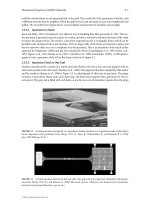
Figure 10.15 shows a schematic of a system that was used to perform and image an electrophoretic sep-
aration in a microfluidic chip. The microchip depicted schematically in Figure 10.15 is commercially
available from Micralyne, Inc., Alberta, Canada. The width and depth of the channels are 50 µm and
20 µmrespectively. The separation channel is 80 mm from the intersection to the waste well (well #4 in
Figure 10.14). A high voltage switching system allows for rapid switching between the injection and sep-
aration voltages and a computer, epifluorescent microscope, and CCD camera are used to image the elec-
trophoretic separation. The system depicted in Figure 10.15 is used to design and characterize
electrokinetic injections; in a typical electrophoresis application, the CCD camera would be replaced with
a point detector (e.g., a photo-multiplier tube) near well #4.
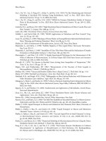
Figure 10.16 shows an injection and separation sequence of 200µM solutions of fluorescein and
Bodipy dyes (Molecular Probes, Inc., Eugene, Oregon). Images 10.16a through 10.16d are each 20 msec
exposures separated by 250 msec. In Figure 16a, the sample is injected applying 0.5 kV and ground to well
#3 and well #2, respectively. The sample volume at the intersection is pinched by flowing buffer from well
#1 and well #4. Once a steady flow condition is achieved, the voltages are switched to inject a small sam-
ple plug into the separation channel. During this separation phase, the voltages applied at well #1 and well
#4 are 2.4 kV and ground respectively. The sample remaining in the injection channel is retracted from
the intersection by applying 1.4 kV to both well #2 and well #3. During the separation, the electric field
strength in the separation channel is about 200 V/cm. The electrokinetic injection introduces an approxi-
mately 400 pL volume of the homogeneous sample mixture into the separation channel, as seen in Figure
10.16b. The Bodipy dye is neutral, and therefore its species velocity is identical to that of the electroos-
motic flow velocity. The relatively high electroosmotic flow velocity in the capillary carries both the neu-
tral Bodipy and negatively charged fluorescein toward well #4. The fluorescein’s negative electrophoretic
mobility moves it against the electroosmotic bulk flow, and therefore it travels more slowly than the
Bodipy dye. This difference in electrophoretic mobilities results in a separation of the two dyes into dis-
tinct analyte bands, as seen in Figures 10.16c and 10.16d. The zeta potential of the microchannel walls for
the system used in this experiment was estimated at Ϫ50 mV from the velocity of the neutral Bodipy dye
[Bharadwaj and Santiago, 2002]. The inherent trade-offs between initial sample plug length, electric field,

Liquid Flows in Microchannels 10-29
CCD
camera
Epifluorescence
microscope
Glass plate
cm
Waste
Waste
Buffer
Sample
Separation
channel
Computer/DAQ
High voltage
switching
system
15 kVDC
power
supply
FIGURE 10.15 Schematic of microfabricated capillary electrophoresis system, flow imaging system, high voltage
control box, and data acquisition computer.
© 2006 by Taylor & Francis Group, LLC
channel geometry, separation channel length, and detector characteristics are discussed in detail by
Bharadwaj et al. (2002). Kirby and Hasselbrink (2004) present a review of electrokinetic flow theory and
methods of quantifying zeta potentials in microfluidic systems. Ghosal (2004) presents a review of band-
broadening effects in microfluidic electrophoresis.
10.2.7 Engineering Considerations: Flow Rate and Pressure of
Simple Electroosmotic Flows
As we have seen, the velocity field of simple electrokinetic flow systems with thin EDLs is approximately

independent of the location in the microchannel and is therefore a “plug flow” profile for any cross-sec-
tion of the channel. The volume flow rate of such a flow is well approximated by the product of the elec-
troosmotic flow velocity and the cross-sectional area of the inner capillary:
Q ϭ Ϫ
.
(10.59)
For the typical case of electrokinetic systems with a bulk ion concentration in excess of about 100 µM
and characteristic dimension greater than about 10 µm, the vast majority of the current carried within
the microchannel is the electromigration current of the bulk liquid. For such typical flows, we can rewrite
the fluid flow rate in terms of the net conductivity of the solution,
σ
,
Q ϭ Ϫ
,
(10.60)
where I is the current consumed, and we have made the reasonable assumption that the electromigration
component of the current flux dominates. The flow rate of a microchannel is therefore a function of the
current carried by the channel and otherwise independent of geometry.
εζ
I
ᎏ
µσ
εζ
EA
ᎏ
µ
10-30 MEMS: Introduction and Fundamentals
3
2
1 4

3
2
1 4
3
2
1 4
3
2
1 4
(a) (b)
(d)(c)
FIGURE 10.16 Separation sequence of Bodipy and fluorescein in a microfabricated capillary electrophoresis system.
The channels shown are 50µm wide and 20 µm deep. The fluoresceine images are 20msec exposures and consecutive
images are separated by 250 msec. A background image has been subtracted from each of the images, and the channel
walls were drawn in for clarity. (Reprinted with permission from Bharadwaj, R., and Santiago, J.G. [2000] unpublished
results, Stanford University.)
© 2006 by Taylor & Francis Group, LLC
Another interesting case is that of an electrokinetic capillary with an imposed axial pressure gradient.
For this case, we can use Equation (10.47) to show the magnitude of the pressure that an electrokinetic
microchannel can achieve. To this end, we solve Equation (10.47) for the maximum pressure generated
by a capillary with a sealed end and an applied voltage ∆V, noting that the electric field and the pressure
gradient can be expressed as ∆V/L and ∆p/L respectively. Such a microchannel will produce zero net flow
but will provide a significant pressure gradient in the direction of the electric field (in the case of a neg-
atively charged wall). Imposing a zero net flow condition Q ϭ
͵
A
u и dA ϭ 0 the solution for pressure gen-
erated in a thin EDL microchannel is then
∆p ϭ Ϫ (10.61)
which shows that the generated pressure will be directly proportional to voltage and inversely propor-

tional to the square of the capillary radius. Equation (10.61) dictates that decreasing the characteristic
radius of the microchannel will result in higher pressure generation. The following section discusses a
class of devices designed to generate both significant pressures and flow rate using electroosmosis.
10.2.8 Electroosmotic Pumps
Electroosmotic pumps are devices that generate both significant pressure and flow rate using electroosmo-
sis through pores or channels. A review of the history and technological development of such electro-
osmotic pumps is presented by Yao and Santiago (2003a). The first electroosmotic pump structure
(generating significant pressure) was demonstrated by Theeuwes in 1975. Other notable contributions
include that of Gan et al. (2000), who demonstrated pumping of several electrolyte chemistries; and Paul et
al. (1998a) and Zeng et al. (2000), who demonstrated of order 10 atm and higher. Yao et al. (2003b) pre-
sented experimentally validated, full Poisson–Boltzmann models for porous electroosmotic pumps. They
demonstrated a pumping structure less than 2cm
3
in volume that generates 33ml/min and 1.3 atm at 100V.
Figure 10.17 shows a schematic of a packed-particle bed electroosmotic pump of the type discussed by
Paul et al. (1998a) and Zeng et al. (2000). This structure achieves a network of submicron diameter
microchannels by packing 0.5–1 micron spheres in fused silica capillaries, using the interstitial spaces in
these packed beds as flow passages. Platinum electrodes on either end of the structure provide applied
potentials on the order of 100 to 10,000 V. A general review of micropumps that includes sections on elec-
troosmotic pumps is given by Laser and Santiago (2004).
8
εζ
∆V
ᎏ
a
2
Liquid Flows in Microchannels 10-31
Particle surfaces and wall
are positively charged
Channel section

upstream of pump
Platinum
electrode
Voltage source: 1-8 kV
Fluidic standoff
for electrode
Downstream
channel section
Flow direction
Liquid flow through
interstitial space
Packed bed (0.5–1 micron
silica spheres)
FIGURE 10.17 Schematic of electrokinetic pump fabricated using a glass microchannel packed with silica spheres.
The interstitial spaces of the packed bed structure create a network of submicron microchannels that can be used to
generate pressures in excess of 5000 psi.
© 2006 by Taylor & Francis Group, LLC
10.2.9 Electrical Analogy and Microfluidic Networks
There is a strong analogy between electroosmotic and electrophoretic transport and resistive electrical
networks of microchannels with long axial-to-radial dimension ratios. As described above, the electroos-
motic flow rate is directly proportional to the current. This analogy holds provided that the previously
described conditions for electric/velocity field similarity also hold. Therefore, Kirkoff’s current and volt-
age laws can be used to predict flow rates in a network of electroosmotic channels given voltage at end-
point nodes of the system. In this one-dimensional analogy, all of the current, and hence all of the flow,
entering a node must also leave that node. The resistance of each segment of the network can be deter-
mined by knowing the cross-sectional area, the conductivity of the liquid buffer, and the length of the
segment. Once the resistances and applied voltages are known, the current and electroosmotic flow rate
in every part of the network can be determined using Equation (10.60).
10.2.10 Electrokinetic Systems with Heterogenous Electrolytes
The previous sections have dealt with systems with uniform properties such as ion-concentrations

(including pH), conductivity, and permittivity. However, many practical electrokinetic systems involve
heterogeneous electrolyte systems. A general transport model for heterogenous electrolyte systems (and
indeed for general electrohydrodynamics) should include formulations for the conservation of species,
Gauss’ law, and the Navier–Stokes equations describing fluid motion [Castellanos, 1998; Melcher, 1981;
Saville, 1997]. The solutions to these equations can in general be a complex nonlinear coupling of these
equations. Such a situation arises in a wide variety of electrokinetic flow systems. This section presents a
few examples of recent and ongoing work in these complex electrokinetic flows.
10.2.10.1 Field Amplified Sample Stacking (FASS)
Sensitivity to low analyte concentrations is a major challenge in the development of robust bioanalytical
devices. Field amplified sample stacking (FASS) is one robust way to carry out on-chip sample precon-
centration. In FASS, the sample is prepared in an electrolyte solution of lower concentration than the
background electrolyte (BGE). The low-conductivity sample is introduced into a separation channel oth-
erwise filled with the BGE. In these systems, the electromigration current is approximately nondivergent
so that ∇ и (
σ
E
ෆ
) ϭ 0, where
σ
is ionic conductivity. Upon application of a potential gradient along the
axis of the separation channel, the sample region is therefore a region of low conductivity (high electric
field) in series with the BGE region(s) of high conductivity (low electric field). Sample ions migrate from
the high-field–high-drift-velocity of the sample region to the low-field–low-drift-velocity region and
accumulate, or stack, at the interface between the low and high conductivity regions.
The seminal work in the analysis of unsteady ion distributions during electrophoresis is that of
Mikkers et al. (1979), who used the Kohlrausch regulating function (KRF) [Beckers and Bocek, 2000;
Kohlrausch, 1897] to study concentration distributions in electrophoresis. There have been several review
papers on FASS, including discussions of on-chip FASS devices, by Quirino et al. (1999), Osborn et al.
(2000), and Chien (2003). FASS has been applied by Burgi and Chien (1991), Yang and Chien (2001), and
Lichtenberg et al. (2001) to microchip-based electrokinetic systems. These three studies demonstrated

maximum signal enhancements of 100-fold over nonstacked assays. More recently, Jung et al. (2003)
demonstrated a device that avoids electrokinetic instabilities associated with conductivity gradients and
achieves a 1,100-fold increase in signal using on-chip FASS. Recent modeling efforts include the work of
Sounart and Baygents (2001), who developed a multicomponent model for electroosmotically driven
separation processes. They performed two-dimensional numerical simulations and demonstrated that
nonuniform electroosmosis in these systems causes regions of recirculating flow in the frame of the mov-
ing analyte plug. These recirculating flows can drastically reduce the efficiency of sample stacking.
Bharadwaj and Santiago (2004) present an experimental and theoretical investigation of FASS dynamics.
Their model analyzes dispersion dynamics using a hybrid analysis method that combines area-averaged,
convective-diffusion equations with regular perturbation methods to provide a simplified equation set
10-32 MEMS: Introduction and Fundamentals
© 2006 by Taylor & Francis Group, LLC
for FASS. They also present model validation data in the form of full-field epifluorescence images quan-
tifying the spatial and temporal dynamics of concentration fields in FASS.
The dispersion dynamics of nonuniform electroosmotic flow FASS systems results in concentration
enhancements that are a strong function of parameters such as electric field, electroosmotic mobility, dif-
fusivity, and the background electrolyte-to-sample conductivity ratio
γ
. At low
γ
and low electroosmotic
mobility, electrophoretic fluxes dominate transport and concentration enhancement increases with
γ
. At
γ
and significant electroosmotic mobilities, increases in
γ
increase dispersion fluxes and lower sample con-
centration rates. The optimization of this process is discussed in detail by Bharadwaj and Santiago (2004).
10.2.10.2 Isotachophoresis

Isothachopheresis [Everaerts et al., 1976] uses a heterogenous buffer to achieve both concentration and
separation of charged ions or macromolecules. Isotachophoresis (ITP) occurs when a sample plug con-
taining anions (or cations) is sandwiched between a trailing buffer and a leading buffer such that all the
sample anions (cations) are slower than the anion (cation) in the leading buffer and faster than all the
anion (cation) in the trailing buffer. When an electric field is applied in this situation, all the sample
anions (cations) will rapidly form distinct zones that are arranged by electrophoretic mobility. In the case
where each sample ion carries the bulk of the current in its respective zone, the KRF states that the final
concentration of each ion will be proportional to its mobility. Because all anions (cations) migrate in distinct
zones, current continuity ensures that they migrate at the same velocity (hence the name isotachophoresis),
resulting in characteristic translating conductivity boundaries. Isotachophoresis in a transient manner is
used as a preconcentration technique prior to capillary electrophoresis; this combination is often referred
to as ITP-CE [Hirokawa, 2003]. Isotachophoresis and ITP-CE in microdevices has been described by
Kaniansky et al. (2000), Vreeland et al. (2003), Wainright et al. (2002), and Xu et al. (2003).
10.2.10.3 Isoelectric Focusing
Isoelectric focusing (IEF) is another electrophoretic technique that utilizes heterogenous buffers to
achieve concentration and separation [Catsimpoolas, 1976; Righetti, 1983]. Isoelectric focusing usually
employs a background buffer containing carrier ampholytes (molecules that can be either negatively
charged, neutral, or positively charged depending on the local pH). The pH at which an amphoteric mol-
ecule is neutral is called the isoelectric point, or pI. Under an applied electric field, the carrier ampholytes
create a pH gradient along a channel or capillary. When other amphoteric sample molecules are intro-
duced into a channel with such a stabilized pH gradient, the samples migrate until they reach the loca-
tion where the pH is equal to the pI of the sample molecule. Thus IEF concentrates initially dilute
amphoteric samples and separate them by isoelectric point. Because of this behavior, IEF is often used as
the first dimension of multidimensional separations. IEF and multidimensional separations employing
IEF have been demonstrated in microdevices by Hofmann et al. (1999), Woei et al. (2002), Li et al. (2004),
Macounova et al. (2001), and Herr et al. (2003).
10.2.10.4 Temperature Gradient Focusing
Another method of sample stacking is temperature gradient focusing (TGF), which uses electrophoresis,
pressure-driven flow, and electroosmosis to focus and separate samples based on electrophoretic mobil-
ity. In TGF, an axial temperature gradient applied axially along a microchannel produces a gradient in

electrophoretic velocity. When opposed by a net bulk flow, charged analytes focus at points where their
electrophoretic velocity and the local, area-averaged liquid velocity sum to zero. The method has been
demonstrated experimentally by Ross and Locascio (2002). A review of various various electrofocusing
techniques is given by Ivory (2000).
10.2.10.5 Electrothermal Flows
A fifth important class of heterogenous electrolyte electrokinetic flows are electrothermal flows. These flows
are generated by electric body forces in the bulk liquid of an electrokinetic flow system with finite temperature
Liquid Flows in Microchannels 10-33
© 2006 by Taylor & Francis Group, LLC
gradients. These flows were first described by Ramos et al. (1998) and have been analyzed by Ramos et al.
(1999) and Green et al. (2000a, 2000b). Work in this area is summarized in the book by Morgan and
Green (2003). These researchers were interested in steady flow-streaming-like behavior observed in microflu-
idic systems with patterned AC electrodes. The devices were designed for dielectrophoretic particle con-
centration and separation. Secondary flows in these systems are generated by the coupling of AC electric
fields and temperature gradients. This coupling creates body forces that can cause order 100 micron per sec-
ond liquid velocities and dominate the transport of particulates in the device. Experimental validation of
these flows has been presented by Green et al. (2000b) and Wang et al. (2004). The latter work used two-
color micron-resolution PIV (Santiago, 1998) to independently quantify liquid and particle velocity fields.
Ramos et al. (1998) presented a linearized theory for modeling electrothermal flows. Electrothermal
forces result from net charge regions in the bulk of an electrolyte with finite temperature gradients.
Temperature gradients are a result of localized Joule heating in the system and affect both local electrical
conductivity
σ
and the dielectric permittivity
ε
. In the Ramos model, ion density is assumed uniform and
the temperature field (and therefore the conductivity and permittivity fields) is assumed known and
steady. The latter assumptions imply a low value of the thermal Peclet number (Probstein, 1994) for the
flow. The general body force on a volume of liquid in this system, f
ෆ

e
can be derived from the divergence
of the Maxwell stress tensor (Melcher, 1981) and written as
f
ෆ
e
ϭ
ρ
E
E
ෆ
Ϫ 0.5|E
ෆ
|
2
∇
ε
Ramos et al. (1998) assume a linear expansion of the form E
ෆ
ϭ E
ෆ
o
ϩ E
ෆ
1
, where E
ෆ
o
is the applied field (sat-
isfying ∇ и E

ෆ
o
ϭ 0) and E
ෆ
1
is the perturbed field, such that |E
o
| ϾϾ |E
1
|. Assuming a sinusoidal applied
field of the form E
ෆ
o
(t) ϭ Re[EE
ෆ
o
exp(j
ω
t)], and substituting this linearization into an expression of the con-
servation of electromigration current (∇ и (
σ
E
ෆ
ϭ 0), yields
∇ и E
ෆ
1
ϭ
,
where higher order terms have been neglected. The (steady, nonuniform) electric charge density is then

ρ
E
ϭ ∇
ε
и
–
E
o
ϩ
ε
∇ и
–
E
1
. This charge density can be combined with the relation for f
ෆ
e
above to solve for
motion of the liquid using the Navier–Stokes equations. Note that this model assumes steady conductiv-
ity and permittivity fields determined solely by a steady temperature field. The electric body force field is
therefore uncoupled from the motion of the liquid.
10.2.10.6 Electrokinetic Flow Instabilities
Electrokinetic instabilities are a sixth interesting example of complex electrokinetic flow in heterogenous
electrolyte systems. Electrokinetic instabilities (EKI) are produced by an unsteady coupling between elec-
tric fields and conductivity gradients. Lin et al. (2004) and Chen et al. (2004) present the derivation of a
model for generalized electrokinetic flow that builds on the general electrohydrodynamics framework
provided by Melcher (1981). This model results in a formulation of the following form:
ϩ v и ∇
σ
ϭ ∇

2
σ,
∇ и (
σ
E
ෆ
) ϭ 0,
∇ и
ε
E
ෆ
ϭ
ρ
E
,
∇ и v ϭ 0,
Re
΂
ϩ v и ∇v
΃
ϭ Ϫ∇p ϩ ∇
2
v ϩ
ρ
E
E
ෆ
.
The first equation governs the development of the unsteady, nonuniform electrolyte conductivity, σ, and
is derived from a summation of the charged species equations. The second equation is derived from a

∂v
ᎏ
∂t
1
ᎏ
Ra
e
∂
σ
ᎏ
∂t
Ϫ(∇
σ
ϩ j
ω
∇
ε
) и E
ෆ
o
ᎏᎏ
σ
ϩ j
ωε
10-34 MEMS: Introduction and Fundamentals
© 2006 by Taylor & Francis Group, LLC
x = 0.2
K
x
= 0.097

LB, slip
LB, no slip
0.5
0
−0.5
0.5
0
−0.5
0 0.11 0.21 0.32
x = 0.5
K
x
= 0.117
K
x
= 0.153
0 0.12 0.24 0.36 0 0.11 0.21 0.32 0.42
0.5
0
−0.5
x = 0.8
u
~
u
~
u
~
~
~~
~

y
~
y
~
y
LB, slip
LB, no slip
LB, slip
LB, no slip
K
x
= 0.097
LB, slip
LB, no slip
0.5
0
−0.5
0.5
0
−0.5
0 0.032 0.057
K
x
= 0.117
K
x
= 0.153
0 0.02 0.04 0.061 0 0.023 0.045 0.066
0.5
0

−0.5
u
~
u
~
u
~
x = 0.8
~
x = 0.5
~
x = 0.2
~
~
y
~
y
~
y
LB, slip
LB, no slip
LB, slip
LB, no slip
COLOR FIGURE 9.5 Velocity profiles for MHD flow in a microchannel. Kn
in
ϭ 0.088, Kn
out
ϭ 0.3, P
in
/P

out
ϭ 2.28,
ε
ϭ H/L ϭ 0.05,
α
ϭ 1, M ϭ 0.1, Ha ϭ 0.054, E
0
ϭ 0.
COLOR FIGURE 9.6 Velocity profiles for MHD flow in a microchannel. Kn
in
ϭ 0.088, Kn
out
ϭ 0.3, P
in
/P
out
ϭ 2.28,
ε
ϭ H/L ϭ 0.05,
α
ϭ 1, M ϭ 0.1, Ha ϭ 5.4, E
0
ϭ 0.
© 2006 by Taylor & Francis Group, LLC
K
x
= 0.097
LB, slip
LB, no slip
0.5

0
−
0.5
0.5
0
−
0.5
0.5
0
−
0.5
u
~
u
~
u
~
x
= 0.2
~
~
y
~
y
~
y
−2
.
10
−4

2
.
10
−4
4
.
10
−4
8
.
10
−4
6
.
10
−4
0
−2
.
10
−4
2
.
10
−4
4
.
10
−4
8

.
10
−4
6
.
10
−4
0
−2
.
10
−4
2
.
10
−4
4
.
10
−4
8
.
10
−4
6
.
10
−4
0
K

x
= 0.153
x = 0.8
~
LB, slip
LB, no slip
K
x
= 0.117
x
= 0.5
~
LB, slip
LB, no slip
COLOR FIGURE 9.7 Ve locity profiles for MHD flow in a microchannel.Kn
in
ϭ 0.088,Kn
out
ϭ 0.3,P
in
/P
out
ϭ 2.28,
ε
ϭ H/L ϭ 0.05,
α
ϭ 1, M ϭ 0.1,Haϭ 54,E
0
ϭ 0.
COLOR FIGURE 10.2 Blood sample cartridge using microfluidic channels.(Reprinted with permission from i-Stat,

East Windsor, NJ, 2000.)
© 2006 by Taylor & Francis Group, LLC
Experiment
t = 0.0 s
t = 1.0 s
t = 1.5 s
t = 2.5 s
t = 5.0 s
Computation
t = 0.0 s
t = 1.0 s
t = 1.5 s
t = 2.5 s
t = 5.0 s
(a) (b)
Quality factor (fluid) in drive axis
Knudsen number
Measurement (LCCC 701)
Continuum flow
Slip flow
Molecular flow
10
10
10
8
10
6
10
4
10

2
10
−2
10
0
10
0
10
2
10
4
10
6
COLOR FIGURE 10.18 Time evolution of electrokinetic flow instability: (a) Experimental data of instability mix-
ing of HEPES buffered 50 µS/cm (red) and 5 µS/cm (blue) conductivity streams [Lin et al., 2004]. At time t ϭ 0.0sec,
a static electric field of E ϭ 50,000V/m is applied in the (horizontal) streamwise direction perpendicular to the ini-
tial conductivity gradients. Image area is 1 mm in the vertical direction and 3.6 mm in the streamwise direction.
Channel depth (into the page) is 100 µm. Small amplitude waves quickly grow and lead to rapid stirring of the ini-
tially distinct buffer streams. (b) Reproduction of dynamics from simplified, 2-D nonlinear numerical computations.
The numerical model well reproduces features of the instability observed in experiments, including wave number and
time scale. Details of this model are given by Lin et al. [2004].
COLOR FIGURE 11.2 Theory and measurements of Couette damping in a tuning fork gyro (Kwok et al. [2005]).
Note that in the high Knudsen number limit, the free molecular approximation predicts the damping more closely,
but that the slip-flow model, though totally inappropriate at this high Kn level, is not too far from the experimental
measurements.
© 2006 by Taylor & Francis Group, LLC
0
0 5 10 15 2520 30
Squeeze number
Non-dimensional forces

0.5
0.4
0.3
0.2
0.1
Damping force
Spring force
COLOR FIGURE 11.5 Solutions to the squeeze-film equation for a rectangular plate. The stiffness and damping
coefficients are presented as functions of the modified squeeze number, which includes a correction due to first-order
rarefaction effects [Blech, 1983; Kwok et al., 2005].
COLOR FIGURE 11.6 Schematic of the MIT Microengine, showing the air path through the compressor, combus-
tor, and turbine. Forward and aft thrust bearings located on the centerline hold the rotor in axial equilibrium, while
a journal bearing around the rotor periphery holds the rotor in radial equilibrium.
COLOR FIGURE 11.13 Geometry of a wave bearing, with the clearance greatly exaggerated for clarity [Piekos, 2000].
© 2006 by Taylor & Francis Group, LLC
−
0.4
−
0.2
−0.6
−0.8
−
1
−0.2
−0.4
−0.8
−
1.5
−
0.5

0
0.5
1
0.8
0.6
0.4
0.2
0
−
1
−1
−
0.6
x
y
z
−
0.4
−
0.6
−0.8
−
1
−2.5
−
2
−
1.5
−1
−

0.5
−0.2
−
0.4
0
0.5
1
0.4
0.2
0
x
z
y
−
0.2
COLOR FIGURE 15.8 Localized controller gains relating the state estimate xˆ inside the domain to the control forcing
u at the point {x ϭ 0, y ϭ Ϫ1, z ϭ 0} on the wall. Visualized are a positive and negative isosurface of the convolution
kernels for (left) the wall-normal component of velocity and (right) the wall-normal component of vorticity.
(Högberg, M., Bewley, T.R., and Henningson, D.S. (2003) “Linear Feedback Control and Estimation of Transition in
Plane Channel Flow,” J. Fluid Mech. 481, pp. 149–75. Reprinted with permission from Elsevier Science.)
0.5
0
−
0.5
−1
−5
0
5
−4
−2

0
2
4
6
8
y
x
z
1
0.5
0
−
0.5
−5
−5
0
5
0
5
10
15
20
−1
y
x
z
1
COLOR FIGURE 15.9 Localized estimator gains relating the measurement error (y Ϫ yˆ) at the point {x ϭ 0,
y ϭ Ϫ1, z ϭ 0} on the wall to the estimator forcing terms v inside the domain. Visualized are a positive and negative
isosurface of the convolution kernels for (left) the wall-normal component of velocity and (right) the wall-normal

component of vorticity. (Högberg, M., Bewley, T.R., and Henningson, D.S. (2003) “Linear Feedback Control and
Estimation of Transition in Plane Channel Flow,” J. Fluid Mech. 481, pp. 149–75. Reprinted with permission from
Elsevier Science.)
© 2006 by Taylor & Francis Group, LLC
(a) ᐉ = 10 (b) ᐉ = 0.5 (c) ᐉ = 0.025
COLOR FIGURE 15.12 Example of the spectacular failure of linear control theory to stabilize a simple nonlinear
chaotic convection system governed by the Lorenz equation. Plotted are the regions of attraction to the desired
stationary point (blue) and to an undesired stationary point (red) in the linearly controlled nonlinear system, and
typical trajectories in each region (black and green, respectively). The cubical domain illustrated is Ω ϭ (Ϫ25, 25)
3
in
all subfigures. For clarity, different viewpoints are used in each subfigure. (Reprinted with permission from Bewley,
T.R. (1999) Phys. Fluids 11, 1169–86. Copyright 1999, American Institute of Physics.)
COLOR FIGURE 15.11 Visualization of the coherent structures of uncontrolled near-wall turbulence at Re
␶
ϭ 180.
Despite the geometric simplicity of this flow (see Figure 15.1), it is phenomenologically rich and is characterized by
a large range of length scales and time scales over which energy transport and scalar mixing occur. The relevant spec-
tra characterizing these complex nonlinear phenomena are continuous over this large range of scales, thus such flows
have largely eluded accurate description via dynamic models of low state dimension. The nonlinearity, the distributed
nature, and the inherent complexity of its dynamics make turbulent flow systems particularly challenging for suc-
cessful application of control theory. (Simulation by Bewley, T.R., Moin, P., and Temam, R. (2001) J. Fluid Mech.
Reprinted with permission of Cambridge University Press.)
© 2006 by Taylor & Francis Group, LLC
1.1
Turbulent flow (average)
Increasing T
+
T
+

= 5
T
+
= 1.5
T
+
= 10
T
+
= 25
T
+
= 50,100
Laminar flow
Drag (normalized)
Time (viscous units)(a)
1.0
0.9
0.8
0.7
0.6
0.5
0.4
0.3
0 500 1000 1500 2000 2500 3000
1
0
Increasing T
+
T

+
= 1.5
T
+
= 5
T
+
= 10
T
+
= 25
T
+
= 50
T
+
= 100
Turbulent kinetic energy (log scale)
(b) Time (viscous units)
0 500 1000 1500 2000 2500 3000
COLOR FIGURE 15.14 Performance of optimized blowing/suction controls for formulations based on minimizing
J
o
(
φ
), case c (see Section 15.9.1.2), as a function of the optimization horizon T
ϩ
.The direct numerical simulations of
turbulent channel flow reported here were conducted at Re
τ

ϭ 100. For small optimization horizons (T
ϩ
ϭ O(1),
sometimes called the “suboptimal approximation”), approximately 20% drag reduction is obtained, a result that can
be obtained with a variety of other approaches. For sufficiently large optimization horizons (T
ϩ
Ն 25), the flow is
returned to the region of stability of the laminar flow, and the flow relaminarizes with no further control effort
required. No other control algorithm tested in this flow to date has achieved this result with this type of flow actua-
tion. (From Bewley, T.R., Moin, P., and Temam, R. (2001) J. Fluid Mech., to appear. Reprinted with permission of
Cambridge University Press.)
Actuator electronics
Control logic
Microflap actuator
Shear-stress sensor
Sensor electronics
COLOR FIGURE 15.20 A MEMS tile integrating sensors, actuators and control logic for distributed flow control
applications. (Developed by Professors Chih-Ming Ho, UCLA, and Yu-Chong Tai, Caltech.)
© 2006 by Taylor & Francis Group, LLC
4
(a)
(b)
2
0
−
2
−4
4
2
0

−2
−4
Secondary
combustion
zone
Primary
combustion
zone
Fuel nozzle
Primary
air jets
Dilution
air jets
Turbine inlet
guide vanes
0.0
0.2
0.4
0.6
0.8
1.0
Scalar
Hurricane Bonnie, Atlantic Ocean
STS-47
(d)
(c)
COLOR FIGURE 15.22 Future interdisciplinary problems in flow control amenable to adjoint-based analysis:
(a) minimization of sound radiating from a turbulent jet (simulation by Prof. Jon Freund, UCLA), (b) maximization
of mixing in interacting cross-flow jets (simulation by Dr. Peter Blossey, UCSD) [Schematic of jet engine combustor
is shown at left. Simulation of interacting cross-flow dilution jets, designed to keep the turbine inlet vanes cool, are

visualized at right.], (c) optimization of surface compliance properties to minimize turbulent skin friction, and
(d) accurate forecasting of inclement weather systems.
© 2006 by Taylor & Francis Group, LLC
conservation of net charge in the limit of fast charge relaxation. As discussed in detail by Lin et al. (2004),
the relaxed charge assumption is consistent with the net neutrality approximation and leads to the con-
dition that electromigration current is at all times conserved. The third equation is Gauss’ law, and the
last two are the Navier–Stokes equations describing fluid velocity with an electrostatic body force of the
form
ρ
E
E
ෆ
. Electrokinetic flow instabilities associated with electrokinetic flows with conductivity gradients
arise from a coupling of these equations. This coupling results in an electric body force (per unit volume)
of the form (
ε
E
ෆ
и ∇
σ
)E
ෆ
,which occurs in regions where local electric field is parallel to the conductivity
gradient. Electrokinetic flows become unstable when the ratio of the characteristic electric body force to
the viscous force in the flow exceeds a critical value [Chen et al., 2004; Lin et al., 2004]. These flows are
unstable even in the limit of vanishing Reynolds number.
Electrokinetic instabilities have been experimentally demonstrated, for various geometric configura-
tions by Oddy et al. (2001), Lin et al. (2004), and Chen et al. (2002, 2004). Figure 10.18 shows both an
experimental visualization and a numerical model of atemporal instability in a microchannel with a con-
ductivity gradient initially orthogonal to the applied electric field [Oddy, 2001]. Chen et al. (2004) show,

Liquid Flows in Microchannels 10-35
Experiment
t = 0.0 s
t = 1.0 s
t = 1.5 s
t = 2.5 s
t = 5.0 s
Computation
t = 0.0 s
t = 1.0 s
t = 1.5 s
t = 2.5 s
t = 5.0 s
(a) (b)
FIGURE 10.18 (See color insert following page 10-34.)Time evolution of electrokinetic flow instability: (a) Experi-
mental data of instability mixing of HEPES buffered 50 µS/cm (red) and 5µS/cm (blue) conductivity streams [Lin et al.,
2004]. At time t ϭ 0.0 sec, a static electric field of E ϭ 50,000V/m is applied in the (horizontal) streamwise direction
perpendicular to the initial conductivity gradients. Image area is 1 mm in the vertical direction and 3.6 mm in the
streamwise direction. Channel depth (into the page) is 100 µm. Small amplitude waves quickly grow and lead to rapid
stirring of the initially distinct buffer streams. (b) Reproduction of dynamics from simplified, 2-D nonlinear numeri-
cal computations. The numerical model well reproduces features of the instability observed in experiments, including
wave number and time scale. Details of this model are given by Lin et al. [2004].
© 2006 by Taylor & Francis Group, LLC
in a slightly different geometry with much shallower channel (11 micron depth), a convective electroki-
netic instability in which spatial growth of disturbances is observed. In both of these experiments thresh-
old electric fields are observed above which the flow becomes unstable and rapid stirring and mixing
occur. Together, the work of Lin et al. (2004) and Chen et al. (2004) describes the basic mechanism behind
electrokinetic instabilities and identifies the critical electric Rayleigh numbers that govern the onset of the
instability. Lin et al. (2004) present linear models for temporal electrokinetic instabilities, a nonlinear
numerical model of the instability, and validation experiments in a long, thin microchannel structure.

Chen et al. (2004) also present experimental results and describe the convective nature of the instability.
The latter work identifies the electroviscous-to-electroosmotic-velocity ratio as the critical value that
demarcates the boundary between convective and absolute instability.
In general, electrokinetic instabilities and flows with unsteady, nonuniform body forces due to cou-
plings between electric fields and conductivity and permittivity gradients are directly relevant to a vari-
ety of on-chip electrokinetic systems. Such complex flow systems include field amplified sample stacking
devices [Bharadwaj and Santiago, 2004; Chien, 2003; Jung et al., 2003]; low-Reynolds number micromix-
ing [Oddy et al., 2001]; multidimensional assay systems [Herr et al., 2003]; and dielectrophoretic devices
[Morgan and Green, 2003]. In general, this complex coupling of applied field and heterogenous elec-
trolyte properties may occur in any electrokinetic system with imperfectly specified sample chemistry.
10.2.11 Practical Considerations
A few practical considerations should be considered in the design, fabrication, and operation of electro-
kinetic microfluidic systems. These considerations include the dimensions of the system, the choice of
liquid and buffer ions, the field strengths used, and the characteristics of the flow reservoirs and inter-
connects. A few examples of these design issues are given here.
In the case of microchannels used to generate pressure, Equation (10.60) shows that a low liquid con-
ductivity is essential for increasing thermodynamic efficiency of an electrokinetic pump because Joule
heating is an important contributor to dissipation [Yao and Santiago, 2003a; Zhao and Liao, 2002]. In
electrokinetic systems for chemical analysis, on the other hand, the need for a stable pH requires a finite
buffer strength, and typical buffer strengths are in the 1–100 mM range. The need for a stable pH there-
fore often conflicts with a need for high fields [Bharadwaj et al., 2002] to achieve high efficiency separa-
tions because of the effects of Joule heating of the liquid.
Joule heating of the liquid in electrokinetic systems can be detrimental in two ways. First, temperature
gradients within the microchannel cause a nonuniformity in the local mobility of electrophoretic parti-
cles because the local viscosity is a function of temperature. This nonuniformity in mobility results in a
dispersion associated with the transport of electrophoretic species [Bosse and Arce, 2000; Grushka et al.,
1989; Knox, 1988]. The second effect of Joule heating is the rise in the absolute temperature of the buffer.
This temperature rise results in higher electroosmotic mobilities and higher sample diffusivities. In
microchip electrophoretic separations, the effect of increased diffusivity on separation efficiency is some-
what offset by the associated decrease in separation time. In addition, the authors have found that an

important limitation to the electric field magnitude in microchannel electrokinetics is that elevated tem-
peratures and the associated decreases in gas solubility of the solution often result in the nucleation of gas
bubbles in the channel. This effect of driving gas out of solution typically occurs well before the onset of
boiling and can be catastrophic to the electrokinetic system because gas bubbles grow and eventually
break the electrical circuit required to drive the flow. This effect can be reduced by outgassing of the solu-
tion and is, of course, a strong function of the channel geometry, buffer conductivity, and the thermal
properties of the substrate material.
Another important consideration in any microfluidic device is the design and implementation of
macro-to-micro fluidic interconnects. Practical implementations of fluidic interconnects span a wide
range of complexity. One common practice (though rarely mentioned in publications) is to simply glue
(e.g., with epoxy and by hand) trimmed plastic pipette tips or short glass tubes around the outlet port on
a fluidic chip to form an end-channel reservoir. Some systems, such as those described by Gray et al.
10-36 MEMS: Introduction and Fundamentals
© 2006 by Taylor & Francis Group, LLC
(1999) for silicon microfluidic chips, incorporate especially microfabricated structures for integrated,
low-dead-volume connections. Krulevitch (2002) describes a set of interconnects applicable to silicone
rubber fluidic systems. Still other systems use Nanoport interconnect fittings commercially available from
Upchurch Scientific. Fluidic interconnects are clearly an area that would benefit from an informed review
of the various advantages and disadvantages of common schemes. These factors include ease of assembly,
typical fabrication yield, dead volume, ability to deal with electrolytic reaction products, and pressure
capacity.
Lastly, an important consideration in electrokinetic experiments is the inadvertent application and/or
generation of pressure gradients in the microchannel. Probably the most common cause of this is a mis-
match in the height of the fluid level at the reservoirs. Although there may not be a mismatch of fluid level
at the start of an experiment, the flow rates created by electroosmotic flow may eventually create a fluid
level mismatch. Also, the fluid level in each reservoir, particularly in reservoirs of 1 mm diameter or less,
may be affected by electrolytic gas generation at each electrode. Because electroosmotic flow rate scales as
channel diameter squared, whereas pressure-driven flow scales as channel diameter to the fourth power,
this effect is greatly reduced by decreasing the characteristic channel diameter. Another common method
of reducing this pressure head effect is to increase the length of the channel for a given cross-section. This

length increase, of course, implies an increase in operating voltages to achieve the same flow rate. A sec-
ond source of pressure gradients is a nonuniformity in the surface charge in the channel. An elegant
closed-form solution for the flow in a microchannel with arbitrary axial zeta potential distribution is pre-
sented by Anderson and Idol (1985). Herr et al. (2000) visualized this effect and offered a simple analyt-
ical expression to the pressure-driven flow components associated with zeta potential gradients in fully
developed channel flows.
10.3 Summary and Conclusions
In microchannels, the flow of a liquid differs fundamentally from that of a gas, primarily due to the effects
of compressibility and potential rarefaction in gases. Significant differences from continuum macroscale
theories have been observed. If experiments are performed with sufficient control and care in channels
with dimensions of the order of tens of microns or larger, the friction factors measured in the range of
accepted laminar flow behavior (i.e., Re Ͻ 2000) agree with classical continuum hydrodynamic theory to
within small or negligible differences [Sharp and Adrian, 2004], and the transition to turbulence occurs
at or near the nominally accepted values for both rectangular and circular microchannels [Liu and
Garimella, 2004; Sharp and Adrian, 2004].
The possibility cannot be ruled out, however, that some physical effects such as roughness or electrical
charge effects are causing a deviation from conventional flow results in certain experiments. Observed
differences may also be due to imperfections in the flow system of the experiment, and because imper-
fections may well occur in real engineering systems, it is essential to understand the sources of the
observed discrepancies in order to avoid them, control them, or factor them into the designs.
Measurement techniques for liquid flows are advancing quickly, both as macroscale methods are adapted
to these smaller scales and as novel techniques are being developed. Further insight into phenomena pres-
ent in the microscale flows, including those due to imperfections in channels or flow systems, is likely to
occur rapidly given the evolving nature of the measurement techniques. Complex, nonlinear channels can
be used efficiently to design for functionality.
Electrokinetics is a convenient and easily controlled method of achieving sample handling and sepa-
rations on a microchip. Because the body force exerted on the liquid is typically limited to a region within
a few nanometers from the wall, the resulting profiles, in the absence of imposed pressure-gradients, are
often plug-like for channel dimensions greater than about 10 µm and ion concentrations greater than
about 10 µM. For simple electroosmotic flows with thin EDLs, low Reynolds number, uniform surface

charge, and zero imposed pressure gradients, the velocity field of these systems is well approximated by
potential flow theory. This significant simplification can, in many cases, be used to predict and optimize
the performance of electrokinetic systems. Further, electrokinetics can be used to generate large pressures
Liquid Flows in Microchannels 10-37
© 2006 by Taylor & Francis Group, LLC
10-38 MEMS: Introduction and Fundamentals
(Ͼ20 atm) on a microfabricated device. In principle, the handling, rapid mixing, and separation of
solutes in less than 1 pL sample volumes should be possible using electrokinetic systems built with cur-
rent microfabrication technologies.
References
Adamson, A.W., and Gast, A.P. (1997) “Physical Chemistry of Surfaces,” 6th ed., John Wiley & Sons, Inc.,
New York.
Alarie, J.P., Jacobson, S.C., Culbertson, C.T., et al. (2000) “Effects of the Electric Field Distribution on
Microchip Valving Performance,” Electrophoresis 21, pp. 100–6.
Anderson, J.L., and Idol, W.K. (1985) “Electroosmosis through Pores with Nonuniformly Charged Walls,”
Chem. Eng. Commn. 38, pp. 93–106.
Arkilic, E.B., Schmidt, M.A., and Breuer, K.S. (1997) “Gaseous Slip Flow in Long Microchannels,” J.
MEMS 6, pp. 167–78.
Arulanandam, S., and Li, D. (2000) “Liquid Transport in Rectangular Microchannels by Electroosmotic
Pumping,” Colloid. Surface. A 161, pp. 89–102.
Auroux, P. A., Iossifidis, D., Reyes, D. R., and Manz, A. (2002) “Micro Total Analysis Systems: 2. Analytical
Standard Operations and Applications,” Anal. Chem. 74, pp. 2637–52.
Baker, D.R. (1995) “Capillary Electrophoresis,” in Techniques in Analytical Chemistry Series, John Wiley &
Sons, Inc., New York.
Beckers, J.L., and Bocek, P. (2000) “Sample Stacking in Capillary Zone Electrophoresis: Principles,
Advantages, and Limitations,” Electrophoresis 21, pp. 2747–67.
Berger, M., Castelino, J., Huang, R., Shah, M., and Austin, R.H. (2001) “Design of a Microfabricated
Magnetic Cell Separator,” Electrophoresis 22, pp. 3883–92.
Bharadwaj, R., and Santiago, J.G. (2005) “Dynamics of Field Amplified Sample Stacking,” in press,
J. Fluid Mech.

Bharadwaj, R., Santiago, J.G., and Mohammadi, B. (2002) “Design and Optimization of On-Chip
Electrophoresis,” Electrophoresis 23, pp. 2729–44.
Bianchi, F., Ferrigno, R., and Girault, H.H. (2000) “Finite Element Simulation of an Electroosmotic-
Driven Flow Division at a T-Junction of Microscale Dimensions,” Anal. Chem. 72, pp. 1987–93.
Blankenstein, G., and Larsen, U.D. (1998) “Modular Concept of a Laboratory on a Chip for Chemical and
Biochemical Analysis,” Biosens. Bioelectron. 13, pp. 427–38.
Bosse, M.A., and Arce, P. (2000) “Role of Joule Heating in Dispersive Mixing Effects in Electrophoretic
Cells: Convective-Diffusive Transport Aspects,” Electrophoresis 21, pp. 1026–33.
Brandner, J., Fichtner, M., Schygulla, U., and Schubert, K. (2000) “Improving the Efficiency of Micro Heat
Exchangers and Reactors,” in Proc. 4th Int’l. Conf. Microreaction Technology, AIChE, 5–9 March,
Atlanta, Georgia, pp. 244–49.
Branebjerg, J., Fabius, B., and Gravesen, P. (1995) “Application of Miniature Analyzers: From Microfluidic
Components to TAS,” in Micro Total Analysis Systems, A. van den Berg and P. Bergveld, eds., Kluwer
Academic Publishers, Dordrecht, pp. 141–51.
Branebjerg, J., Gravesen, P., Krog, J.P., and Nielsen, C.R. (1996) “Fast Mixing by Lamination,” in Proc. 9th
Annual Workshop of Micro Electro Mechanical Systems, San Diego, California, 11–15 February, pp.
441–46.
Bridgman, P.W. (1923) “The Thermal Conductivity of Liquids Under Pressure,” American Academy of
Arts and Sciences 59, pp. 141–59.
Brody, J.P., Yager, P., Goldstein, R.E., and Austin, R.H. (1996) “Biotechnology at Low Reynolds Numbers,”
Biophys. J. 71, pp. 3430–41.
Bruin, G.J.M. (2000) “Recent Developments in Electrokinetically Driven Analysis on Microfabricated
Devices,” Electrophoresis 21, pp. 3931–51.
Brutin, D., and Tadrist, L. (2003) “Experimental Friction Factor of a Liquid Flow in Microtubes,” Phys.
Fluids 15, pp. 653–61.
© 2006 by Taylor & Francis Group, LLC
Burgi, D.S., and Chien, R.L. (1991) “Optimization of Sample Stacking for High Performance Capillary
Electrophoresis,” Anal. Chem. 63, pp. 2042–47.
Burgreen, D., and Nakache, F.R. (1964) “Electrokinetic Flow in Ultrafine Capillary Slits,” J. Phys. Chem.
68, pp. 1084–91.

Castellanos, A. (1998) Electrohydrodynamics, New York, Springer-Verlag Wien.
Catsimpoolas, N. (1976) Isoelectric Focusing, New York, Academic Press.
Celata, G.P., Cumo, M., Guglielmi, M., and Zummo, G. (2002) “Experimental Investigation of Hydraulic
and Single-Phase Heat Transfer in a 0.130-mm Capillary Tube,” Microscale Thermophys. Eng. 6,
p. 85–97.
Chen, C H., Lin, H., Santiago, J.G., and Lele, S.K. (2005) “Convective and absolute Electrokinetic Flow
Instability,” with conductivity gradients J. Fluid Mech, 524, pp. 263–303.
Chen, Z., Milner, T.E., Dave, D., and Nelson, J.S. (1997) “Optical Doppler Tomographic Imaging of Fluid
Flow Velocity in Highly Scattering Media,” Opt. Lett. 22, pp. 64–66.
Chien, R. (2003) “Sample Stacking Revisited: A Personal Perspective,” Electrophoresis 24, pp. 486–97.
Cho, S.K., and Kim, C J. (2003), “Particle Separation and Concentration Control for Digital Microfluidic
Systems,” Proc Sixteenth Ann. Conf. on MEMS, MEMS-03, 19–23 January, Kyoto, Japan, pp. 686–89.
Choi, C H., Westin, K.J.A., and Breuer, K.S. (2003) “Apparent Slip Flows in Hydrophilic and
Hydrophobic Microchannels,” Phys. Fluids 15, pp. 2897–2902.
Choi, S.B., Barron, R.F., and Warrington, R.O. (1991) “Fluid Flow and Heat Transfer in Microtubes,” in
DSC-Vol. 32, Micromechanical Sensors, Actuators and Systems, ASME Winter Annual Meeting,
Atlanta, Georgia, pp. 123–34.
Chou, C F., Austin, R.H., Bakajin, O., Tegenfeldt, J.O., Castelino, J.A., Chan, S.S., Cox, E.C., Craighead, H.,
Darnton, N., Duke, T., Han, J., and Turner, S. (2000) “Sorting Biomolecules with Microdevices,”
Electrophoresis 21, pp. 81–90.
Cui, H H., Silber-Li, Z H., and Zhu, S N. (2004) “Flow Characteristics of Liquids in Microtubes Driven
by a High Pressure,” Phys. Fluids 16, pp. 1803–10.
Cummings, E.B., and Singh, A.K. (2003) “Dielectrophoresis in Microchips Containing Arrays of
Insulating Posts: Theoretical and Experimental Results,” Anal. Chem. 75, pp. 4724–31.
Cummings, E.B., Griffiths, S.K., and Nilson, R.H. (1999) “Irrotationality of Uniform Electroosmosis,”
in SPIE Conference on Microfluidic Devices and Systems II, 20–22 September, Santa Clara, California,
3877, pp. 180–89.
Cummings, E.B., Griffiths, S.K., Nilson, R.H., et al. (2000) “Conditions for Similitude Between the Fluid
Velocity and Electric Field in Electroosmotic Flow,” Anal. Chem. 72, pp. 2526–32.
Darbyshire, A.G., and Mullin, T. (1995) “Transition to Turbulence in Constant-Mass-Flux Pipe Flow,”

J. Fluid Mech. 289, pp. 83–114.
Devasenathipathy, S., and Santiago, J.G. (2000) unpublished results, Stanford University, Stanford,
California, October.
Devasenathipathy, S., Santiago, J.G., and Takehara, K. (2002) “Particle Tracking Techniques for
Electrokinetic Microchannel Flows,” Anal. Chem. 74, pp. 3704–13.
Devasenathipathy, S., Santiago, J.G., Wereley, S.T., Meinhart, C. D., and Takehara, K. (2003) “Particle
Imaging Techniques for Microfabricated Fluidic Systems,” Exp. Fluids 34, pp. 504–14.
Dutta, P., Beskok, A., and Warburton, T.C. (2002) “Electroosmotic Flow Control in Complex
Microgeometries,” J. Microelectromech. Sys. 11, pp. 36–44.
Ermakov, S.V., Jacobson, S.C., and Ramsey, J.M. (2000) “Computer Simulations of Electrokinetic
Injection Techniques in Microfluidic Devices,” Anal. Chem. 72, pp. 3512–17.
Everaerts, F.M., Beckers, J.L., and Verheggen, T.P.E.M. (1976) Isotachophoresis: Theory, Instrumentation,
and Applications, Elsevier, New York.
Fiechtner, G.J., and Cummings, E.B. (2003) “Faceted Design of Channels for Low-Dispersion Electrokinetic
Flows in Microfluidics Systems,” Anal. Chem. 75, pp. 4747–55.
Flockhart, S.M., and Dhariwal, R.S. (1998) “Experimental and Numerical Investigation into the Flow
Characteristics of Channels Etched in <100> Silicon,” J. Fluids Eng. 120, pp. 291–95.
Liquid Flows in Microchannels 10-39
© 2006 by Taylor & Francis Group, LLC
Fu, L M., Yang, R J., Lin, C H., Pan, Y J., and Lee, G B. (2004) “Electrokinetically Driven Micro Flow
Cytometers with Integrated Fiber Optics for On-Line Cell/Particle Detection,” Anal. Chim. Acta
507, pp. 163–69.
Gad-el-Hak, M. (1999) “The Fluid Mechanics of Microdevices: The Freeman Scholar Lecture,” J. Fluids.
Eng. 121, pp. 5–33.
Galambos, P., and Forster, F.K. (1998) “Micro-Fluidic Diffusion Coefficient Measurement,” in Micro Total
Analysis Systems, D.J. Harrison and A. van den Berg, eds., Kluwer Academic Publishers, Dordrecht,
pp. 189–192.
Gan, W., Yang, L., He, Y., Zeng, R., Cervera, M.L., and d. l. Guardia, M. (2000) Talanta 51, p. 667.
Ghosal, S. (2002) “Lubrication Theory for Electro-Osmotic Flow in a Microfluidic Channel of Slowly
Varying Cross-Section and Wall Charge,” J. Fluid Mech. 459, pp. 103–28.

Ghosal, S. (2004) “Fluid Mechanics of Electroosmotic Flow and its Effects on Band Broadening in
Capillary Electrophoresis,” Electrophoresis 25, pp. 214–28.
Glückstad, J. (2004) “Sorting Particles with Light,” Nat. Mater. 3, pp. 9–10.
Gray, B., Jaeggi, D., Mourlas, N., van Drieenhuizen, B., Williams, K., Maluf, N., and Kovacs, G.S. (1999)
“Novel interconnection technologies for integrated microfluidic Systems,” Sensor. Actuator. A-
Phys. 77, pp. 57–65.
Green, N.G., Ramos, A ,Gonzales, A., Castellanos, A. and Morgan, H. (2000a) “Electric-Field-Induced Fluid
Flow on Microelectrodes: The Effects of Illumination,” J. Phys. D: Appl. Phys. 33, pp. L13–17.
Green, N.G., Ramos, A., Gonzales, A., Morgan, H., and Castellanos, A. (2000b) “Fluid Flow Induced by
Non-Uniform AC Electric Fields in Electrolytes on Microelectrodes: Part 1, Experimental
Measurements,” Phys. Rev. E 61, pp. 4011–18.
Griffiths, S.K., and Nilson, R.H. (2001) “Low Dispersion Turns and Junctions for Microchannel Systems,”
Anal. Chem. 73, pp. 272–78.
Grushka, E., McCormick, R.M., and Kirkland, J.J. (1989) “Effect of Temperature Gradients on the
Efficiency of Capillary Zone Electrophoresis Separations,” Anal. Chem. 61, pp. 241–46.
Hagen, G. (1839) On the Motion of Water in Narrow Cylindrical Tubes, (German) Pogg. Ann. 46, p. 423.
Hanks, R.W., and Ruo, H C. (1966) “Laminar-Turbulent Transition in Ducts of Rectangular Cross
Section,” I&EC Fundamentals 5, p. 558–61.
Harley, J.C., Huang, Y., Bau, H.H., and Zemel, J.N. (1995) “Gas Flow in Micro-channels,” J. Fluid Mech.
284, pp. 257–74.
Hayes, M., Kheterpal, I., and Ewing, A. (1993) “Effects of Buffer pH on Electoosmotic Flow Control by an
Applied Radial Voltage for Capillary Zone Electrophoresis,” Anal. Chem. 65, pp. 27–31.
Henry, D.C. (1948) “The Electrophoresis of Suspended Particles: 4, The Surface Conductivity Effect,”
Trans. Faraday Soc. 44, pp. 1021–26.
Herr, A.E., Molho, J.I., Drouvalakis, K.A., Mikkelsen, J.C.,Utz, P.J., Santiago, J.G., and Kenny, T.W. (2003)
“On-Chip Coupling of Isoelectric Focusing and Free Solution Electrophoresis for Multi-
Dimensional Separations,” Anal. Chem. 75, pp. 1180–87.
Herr, A.E., Molho, J.I., Santiago, J.G., et al. (2000) “Electroosmotic Capillary Flow with Nonuniform Zeta
Potential,” Anal. Chem. 72, pp. 1053–57.
Hiemenz, P.C., and Rajagopalan, R. (1997) “Principles of Colloid and Surface Chemistry,” 3rd ed., Marcel

Dekker, Inc., New York.
Hirokawa, T., Okamoto, H., and Gas, B. (2003) “High-Sensitive Capillary Zone Electrophoresis Analysis
Bb Electrokinetic Injection with Transient Isotachophoretic Preconcentration: Electrokinetic
Supercharging,” Electrophoresis 24, pp. 498–504.
Hitt, D.L., and Lowe, M.L. (1999) “Confocal Imaging of Flows in Artificial Venular Bifurcations,” Trans.
ASME J. Biomech. Eng. 121, pp. 170–77.
Ho, C M., and Tai, Y C. (1998) “Micro-Electro-Mechanical Systems (MEMS) and Fluid Flows,” Annu.
Rev. Fluid Mech. 30, pp. 579–612.
Hofmann, O., Che, D.P., Cruickshank, K.A., and Muller, U.R. (1999) “Adaptation of Capillary Isoelectric
Focusing to Microchannels on a Glass Chip,” Anal. Chem. 71, pp. 678–86.
10-40 MEMS: Introduction and Fundamentals
© 2006 by Taylor & Francis Group, LLC
Hsieh, S S., Lin, C Y., Huang, C F., and Tsai, H H. (2004) “Liquid Flow in a Micro-Channel,”
J. Micromech. Microeng. 14, pp. 436–45.
Huang, T., Tsai, P., Wu, Ch., and Lee, C. (1993) “Mechanistic Studies of Electroosmotic Control at the
Capillary-Solution Interface,” Anal. Chem. 65, pp. 2887–93.
Hunter, R.J. (1981) “Zeta Potential in Colloid Science,” Academic Press, London.
Israelachvili, J.N. (1986) “Measurement of the Viscosity of Liquids in Very Thin Films,” J. Coll. Interface
Sci. 110, pp. 263–71.
Ivory, C.F. (2000). “A Brief Review of Alternative Electrofocusing Techniques,” Separ. Sci. Technol. 35, pp.
1777–93.
Jacobson, S.C., Hergenroder, R., Moore, A.W. Jr., and Ramsey, J.M. (1994) “Precolumn Reactions with
Electrophoretic Analysis Integrated on a Microchip,” Anal. Chem. 66, pp. 4127–32.
Janson, S.W., Helvajian, H., and Breuer, K. (1999) “MEMS, Microengineering and Aerospace Systems,” in
30th AIAA Fluid Dyn. Conf., 28 June–1 July, Norfolk, Virginia, AIAA 99-3802.
Jiang, X.N., Zhou, Z.Y., Yao, J., Li, Y., and Ye, X.Y. (1995) “Micro-Fluid Flow in Microchannel,” in
Transducers ’95:Eurosensor IX, 8th Intl. Conf. on Solid-State Sensors and Actuators, and
Eurosensors IX, 25–29, 1995, in Stockholm, Sweden, pp. 317–20.
Judy, J., Maynes, D., and Webb, B.W. (2002) “Characterization of Frictional Pressure Drop for Liquid
Flows through Microchannels,” Int. J. Heat Mass Transf. 45, pp. 3477–89.

Jung, B., Bharadwaj, R., and Santiago, J.G. (2003) “Thousand-Fold Signal Increase Using Field Amplified
Sample Tacking for On-Chip Electrophoresis,” Electrophoresis 24, pp. 3476–83.
Kaniansky, D., Masar, M., Bielcikova, J., Ivanyi, F., Eisenbeiss, F., Stanislawski, B., Grass, B., Neyer, A., and
Johnck, M. (2000) “Capillary Electrophoresis Separations on a Planar Chip with the Column-
Coupling Configuration Separation Channels,” Anal. Chem. 72, pp. 3596–3604.
Khaledi, M.G. (1998) “High-Performance Capillary Electrophoresis,” in Chemical Analysis: A Series of
Monographs on Analytical Chemistry and its Applications, J.D. Winefordner, ed., p. 146, John Wiley &
Sons, Inc., New York.
Kirby, B.J. (2004) “Zeta Potential of Microfluidic Substrates: 1. Theory, Experimental Techniques, and
Effects on Separations,” Electrophoresis 25, pp. 187–202.
Kitahara, A., and Watanabe, A. (1984) Electrical Phenomena at Interfaces: Fundamentals, Measurements,
and Applications, Surfactant Science Series 15, Marcel Dekker, New York.
Knox, J.H. (1988) “Thermal Effects and Band Spreading in Capillary Electro-Separation,”
Chromatographia 26, pp. 329–37.
Kohlrausch, F. (1897) “Über Konzentrations Verschicbungen durch Electrolyse im Innern von Lösungen
and Losungsgemischen,” Ann. Phys. (Leipzig) 62, pp. 209–39.
Koo, J., and Kleinstreuer, C. (2003) “Liquid Flow in Microchannels: Experimental Observations and
Computational Analyses of Microfluidics Effects,” J. Micromech. Microeng. 13, pp. 568–79.
Koutsiaris, A.G., Mathiouslakis, D.S., and Tsangaris, S. (1999) “Microscope PIV for Velocity-Field
Measurement of Particle Suspensions Flowing inside Glass Capillaries,” Meas. Sci. Technol. 10,
pp. 1037–46.
Krulevitch, P., Bennett, W., Hamilton, J., Maghribi, M., and Rose, K. (2002) “Polymer-Based Packaging
Platform for Hybrid Microfluidic Systems,” Biomed. Microdevices 4, pp. 301–8.
Landers, J.P. (1994) Handbook of Capillary Electrophoresis, CRC Press, Boca Raton, FL.
Lanzillotto, A M., Leu, T S., Amabile, M., and Wildes, R. (1996) “An Investigation of Microstructure and
Microdynamics of Fluid Flow in MEMS,” in AD-Vol. 52, Proc. of ASME Aerospace Division,
Atlanta, Georgia, pp. 789–96.
Laser, D., and Santiago, J.G. (2004) “A Review of Micropumps,” J. Micromech. Microeng. 14, pp. R35–R64.
Lee, G B., Hung, C I., Ke, B J., Huang, G R., Hwei, B H., and Lai, H F. (2001) “Hydrodynamic
Focusing for a Micromachined Flow Cytometer,” J. Fluids Eng. 123, pp. 672–79.

Lee, G B., Lin, C H., and Chang, G L. (2003) “Micro Flow Cytometers with Buried SU-8/SOG Optical
Waveguides,” Sensor. Actuator. A 103, pp. 165–70.
Levich, V. (1962) Physicochemical Hydrodynamics, Prentice-Hall, Englewood Cliffs, N.J.
Liquid Flows in Microchannels 10-41
© 2006 by Taylor & Francis Group, LLC
Li, Y., Buch, J.S., Rosenberger, F., DeVoe, D.L., and Lee, C.S. (2004) “Integration of Isoelectric Focusing
with Parallel Sodium Dodecyl Sulfate Gel Electrophoresis for Multidimensional Protein
Separations in a Plastic Microfluidic Network,” Anal. Chem. 76, pp. 742–48.
Li, Z X., Du, D X., and Guo, Z Y. (2003) “Experimental Study on Flow Characteristics of Liquid in
Circular Microtubes,” Microscale Thermophys. Eng. 7, pp. 253–65.
Lichtenberg, J., Verpoorte, E., and de Rooij, N.F. (2001) “Sample Preconcentration by Field Amplification
Stacking for Microchip-Based Capillary Electrophoresis,” Electrophoresis 22, pp. 258–71.
Lin, H., Storey, B., Oddy, M., Chen, C H., and Santiago, J.G. (2004) “Instability of Electrokinetic
Microchannel Flows with Conductivity Gradients,” Phys. Fluids 16, pp. 1922–35.
Liu, D., and Garimella, S.V. (2004) “Investigation of Liquid Flow in Microchannels,” J. Thermophys. Heat
Transf. 18, pp. 65–72.
Liu, R.H., Stremler, M.A., Sharp, K.V., Olsen, M.G., Santiago, J.G., Adrian, R.J., Aref, H., and Beebe, D.J.
(2000) “Passive Mixing in a Three-Dimensional Serpentine Microchannel,” J. MEMS 9, pp. 190–97.
MacInnes, J., Du, X., and Allen, R. (2003) “Prediction of Electrokinetic and Pressure Flow in a
Microchannel T-Junction,” Phys. Fluids 15, pp. 1992–2005.
Macounova, K., Cabrera, C.R., and Yager, P. (2001) “Concentration and Separation of Proteins in
Microfluidic Channels on the Basis of Transverse IEF,” Anal. Chem. 73, pp. 1627–33.
Mala, G.M., and Li, D. (1999) “Flow Characteristics of Water in Microtubes,” Int. J. Heat Fluid Flow 20,
pp. 142–48.
Manz, A., Effenhauser, C.S., Burggraf, N., et al. (1994) “Electroosmotic Pumping and Electrophoretic
Separations for Miniaturized Chemical Analysis Systems,” J. Micromech. Microeng. 4, pp. 257–65.
Maynes, D., and Webb, A.R. (2002) “Velocity Profile Characterization in Sub-Millimeter Diameter Tubes
Using Molecular Tagging Velocimetry,” Exp. Fluids 32, pp. 3–15.
Meinhart, C.D., Wereley, S.T., and Santiago, J.G. (1999) “PIV Measurements of a Microchannel Flow,”
Exp. Fluids 27, pp. 414–19.

Melcher, J.R. (1981) Continuum Electromechanics. MIT Press, Boston.
Merkle, C.L., Kubota, T., and Ko, D.R.S. (1974) “An Analytical Study of the Effects of Surface Roughness
on Boundary-layer Transition,” AF Office of Scien. Res. Space and Missile Sys. Org., AD/A004786.
Mikkers, F.E.P., Everaerts, F.M., and Verheggen, T. (1979) “High-Performance Zone Electrophoresis,”
J. Chromatogr. 169, pp. 11–20.
Mirowski, W., Moreland, J., Russek, S.E., and Donahue, M.J. (2004) “Integrated Microfluidic Isolation
Platform for Magnetic Particle Manipulation in Biological Systems,” Appl. Phys. Lett. 84,
pp. 1786–88.
Mohammadi, B., Molho, J.I., and Santiago, J.G. (2003) “Incomplete Sensitivities for the Design of
Minimal Dispersion Fluidic Channels,” Comput. Meth. Appl. Mech. Eng. 192, pp. 4131–45.
Morgan, H., and Green, N.G. (2003) AC Electrokinetics: Colloids and Nanoparticles, Research Studies Press
Ltd., Baldock, England.
Morini, G.L. (2004) “Laminar-to-Turbulent Flow Transition in Microchannels,” Microscale Thermophys.
Eng. 8, pp. 15–30.
Myung-Suk, C., and Kwak, H.W. (2003) “Electrokinetic Flow and Electroviscous Effect in a Charged Slit-
Like Microfluidic Chan with Nonlinear Poisson-Boltzmann Field,” Korea-Australia Rheol. J. 15,
pp. 83–90.
Nguyen, N T., and Wereley, S. (2002) Fundamentals and Applications of Microfluidics, Artech House,
Norwood, MA.
Novotny, E.J., and Eckert, R.E. (1974) “Rheological Properties of Viscoelastic Fluids from Continuous
Flow through a Channel Approximating Infinite Parallel Plates,” Trans. Soc. Rheol. 18, pp. 1–26.
Obot, N.T. (2002) “Toward a Better Understanding of Friction and Heat/Mass Transfer in Microchannels:
A Literature Review,” Microscale Thermophys. Eng. 6, pp. 155–73.
Oddy, M., and Santiago, J.G. (2004) “Alternating Electric Field Measurements of Particle Zeta-Potentials
in a Microchannel,” J. Colloid Interface Sci. 269, pp. 192–204.
10-42 MEMS: Introduction and Fundamentals
© 2006 by Taylor & Francis Group, LLC