The MEMS Handbook Introduction & Fundamentals (2nd Ed) - M. Gad el Hak Part 11 ppsx

the alignment process presented here takes place in the time range of a second. A similar mechanism,
by which a hard contact lens centers itself over the cornea in a human eye, was discussed by Moriarty and
Terrill (1996).
The centrifugal spinning of volatile solutions is a convenient and efficient means of coating planar
solids with thin films. This process, known as spin coating, has been widely used in many technological
processes, such as deposition of dielectric layers onto silicon wafers in the microelectronic industry, for-
mation of ultrathin antireflective coatings for deep UV lithography, and others. Two important stages of
Physics of Thin Liquid Films 12-5
FIGURE 12.3 Deposition of water onto a patterned surface with hydrophilic microchannels with corners. The width
of the channel in the corner region increases from channel (a) to channel (e). Time and therefore the volume of the
condensate increase from top to bottom. When a microchannel undergoes a morphological change of its shape, the
drop moves to the corner to maximize the contact area with the hydrophilic part of the substrate. (Reprinted with
permission from Herminghaus et al. (2000).)
© 2006 by Taylor & Francis Group, LLC
12-6 MEMS: Introduction and Fundamentals
FIGURE 12.4 Infrared images of various states as seen in the experiments. The temperature increases with increas-
ing brightness, so warm depression regions are white (except in (c)) and cool elevated regions are dark. Each image
has its own brightness, so temperatures in different images cannot be compared. (a) A localized depression (dry spot)
with a helium gas layer and d ϭ 0.025 cm. (b) A localized elevation (high spot) with an air gas layer and d ϭ 0.037 cm.
(c) A dry spot with hexagons in the surrounding region and d ϭ 0.025 cm. (d) Hexagons with an air gas layer and
d ϭ 0.045 cm. For more detail refer to the source. (Reprinted with permission from VanHook et al. (1997).)
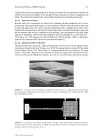
t = 0:00 min 10:30 min 13:50 min
t = 15:30 min 17:10 min 20:15 min
FIGURE 12.5 The evolution of a localized depression and formation of a dry spot in silicone oil of depth
d ϭ 0.0267 Ϯ 0.0008 cm and helium in the gas layer. At t ϭ 0 (an arbitrary starting point) there is negligible defor-
mation of the interface. The liquid layer begins to form a localized depression (the white circle), and in 15 minutes
the interface has ruptured (h
min
→ 0) and formed a dry spot. The dry spot continues to grow for several more min-
utes before saturating. Bright (dark) regions are hot (cool) because they are closer (farther) to (from) the heater. All
images have the same intensity scaling. (Reprinted with permission from VanHook et al. (1997).)

© 2006 by Taylor & Francis Group, LLC
the process are usually considered. The first stage occurs shortly after the liquid volume is delivered to the
disk surface rotating usually at the speed of 1000–10,000r/min. At the beginning of this stage the liquid
film is relatively thick (usually greater than 500 microns). The film thins mainly because of radial drainage
under the influence of centrifugal forces. Inertial forces are important and can lead to the appearance of
instabilities of the spinning film. The second stage occurs when the film has thinned to the point where
inertia is no longer important (film thickness usually less than 100 microns), and the flow slows down
considerably, but deformations of the fluid interface may still be present because of the instabilities that
appeared during the first stage. The film continues to thin mainly because of solvent evaporation until the
Physics of Thin Liquid Films 12-7
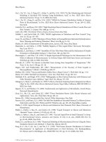
FIGURE 12.6 Photographs of C4 bonding based on self-alignment mechanism. (a) Layout of the chip (4 mm by
4 mm) which consists of four solder joints made of 63Sn37Pb. The upper chip is not aligned with the lower one, as
can be seen from the position of the upper cross relative to four squares at the lower chip. Initial misalignment is 150
microns. (b) An enlarged picture of one of the solder joints at the initial moment. (c) An intermediate stage. (d) The
final position. (e) A side view showing the cross-section of the solder joint at the final stage. (Reprinted with permis-
sion from Salalha et al. (2000).)
© 2006 by Taylor & Francis Group, LLC
solvent becomes depleted, and the film solidifies and ceases to flow. Such problems are discussed in the
sections on isothermal films and phase changes.
Numerous applications relevant for MEMS involve the dynamics of liquid films or drops. This area is in
constant progress and new exciting developments are often reported in the literature. Knight et al. (1998)
describes a new method of enhancement and control of nanoscale fluid jets.They demonstrated this method
with a design of a continuous-flow mixer capable of mixing flow rates of nanoliters per second within the time
scale of 10 microseconds. Such a mixer can be useful in nanofabrication techniques and serve as an essen-
tial part of a microreactor built on a chip.
Spatially controlled changes in the chemical structure of a solid substrate can guide a deposited liquid
along the substrate. Ichimura et al. (2000) reported their experimental results showing the possibility of
reversible guidance of liquid motion by light irradiation of a photoresponsive solid substrate. Asymmetric
irradiation of the solid surface with blue light led to movement of a 2 microliter olive oil droplet with a
typical speed of 35 microns/sec. A similar irradiation with a homogeneous blue light stopped the movement

of the droplet completely. The speed of the droplet and the direction of its movement were adjustable to
the conditions of such irradiation. The phenomenon described has a potential applicability in design of
microreactors and microchips.
Schaeffer et al. (2000) proposed a new technique of creating and replicating lateral structures in films
on submicron length scales. This technique is based on the fact that lateral gradients of the electric field
applied in the vicinity of the film interface induce variations of surface tension and thus lead to the elec-
trocapillary effect. The electrocapillary effect is similar to the thermocapillary effect previously mentioned
and is addressed more thoroughly in the section on thermal effects. The electrocapillary effect triggering
the electrocapillary instability of the film results in formation of ordered patterns on the film interface
and focusing of the interfacial troughs and peaks in the desired locations following the master pattern of
the electrodes. Schaeffer et al. (2000) reported the replication of patterns of lateral dimensions of order
140 nanometers while employing this technique. A complete investigation of the electrocapillary insta-
bility of thin liquid films has not yet appeared in the literature. Lee and Kim (2000) presented a liquid
micromotor and liquid–metal droplets rotating along a microchannel loop driven by continuous elec-
trowetting (CEW) phenomenon based on the electrocapillary effect. They identified and developed key
technologies to design, manufacture, and test the first MEMS devices employing CEW.
A mathematical treatment of this and other phenomena must consider that the interface of the film lying
or flowing on a solid surface is partially or entirely a free boundary whose configuration evolving both tem-
porally and spatially must be determined as an integral part of the solution of the governing equations.
This renders the problem too difficult and often almost intractable analytically, which might lead researchers
to rely on computing only. Computing also becomes complicated because of the free-boundary character
of the problem which requires a careful design of adequate numerical methods.
Another property of such mathematical problems is their strong inherent nonlinearity, which is present
in both governing equations and boundary conditions. This nonlinearity of the problem presents another
complexity. Consideration of coupled phenomena, such as those previously mentioned, requires compact
description of simultaneous instabilities that interact in intricate ways. This compact form must be tract-
able and, at the same time, complex enough to retain the main features of the problem at hand.
The most appropriate analytical method of dealing with the above complexities is to analyze only long
scale phenomena, in which the characteristic lateral length scales are much larger than the average film thick-
ness, the flow-field and temperature variations along the film are much more gradual than those normal to

it, and the time variations are slow. Similar theories arise in a variety of areas of classical physics: shallow-water
theory for water waves, lubrication theory in viscous flows, slender-body theory in aerodynamics, and in
dynamics of jets [e.g., Yarin, 1993]. In all of these examples, a geometrical disparity is used to practically
separate the variables and to simplify the analysis. In thin viscous films, most rupture and instability phe-
nomena occur on long scales, and a long-wave approach explained later is very useful.
The long-wave theory approach is based on the asymptotic reduction of the governing equations and
boundary conditions to a simplified system, which consists often, but not always, of a single nonlinear
partial differential equation formulated in terms of the local thickness of the film varying in time and
12-8 MEMS: Introduction and Fundamentals
© 2006 by Taylor & Francis Group, LLC
space. The rest of the unknowns (i.e., the fluid velocity, pressure, temperature, etc.) are determined
via functionals of the solution of this differential equation usually called evolution equation. The notori-
ous complexity of a free-boundary problem thus is removed. The corresponding penalty is, however,
the presence of the strong nonlinearity in the evolution equation(s) and the higher-order spatial derivatives
(usually up to the fourth) appearing there. A simplified linear stability analysis of the problem can
be carried out based on the resulting evolution equation. A weakly nonlinear analysis of the problem
is also possible through that equation. However, the fully nonlinear analysis that allows one to study
finite-amplitude deformations of the film interface must be performed numerically. Numerical solution
of the evolution equation is incomparably less difficult than that of the original, free-boundary problem.
Several encouraging verifications of the long-wave theory versus the experimental results have appeared
in the literature. Burelbach et al. (1990) carried out a series of experiments in an attempt to check the
long-wave theory of Tan et al. (1990) for steady thermocapillary flows induced by non-uniform heating
of the solid substrate. The measured steady shapes were favorably tested against theoretical predictions
for layers less than 1 mm thick under moderate heating conditions. However, the relative error was large
for conditions near rupture, where the long-wave theory is formally invalid [Burelbach et al., 1988], but
in all other cases the predicted and measured values of the minimal film thickness agreed within 20%.
The theory (see Equation (3.6) of [Tan et al., 1990]) also predicts rupture when the parameter L exceeds
a certain critical value and predicts steady patterns otherwise. Experimental results (see Figure 1 of
[Burelbach et al., 1990]) show that L is an excellent qualitative indicator of whether the film ruptures.
VanHook et al. (1995, 1997) performed experiments on the onset of the long-wavelength insta-

bility in thin layers of silicone oil of varying thickness, aspect ratios, and transverse temperature
gradients across the layer. A formation of “dry spots” at randomly varying locations was found above the
critical temperature difference across the layer in qualitative agreement with corresponding numerical
simulations. The experimental support for the theoretical results is discussed in various sections of this
chapter.
Another test for the validity of an asymptotic theory, such as the long-wave theory presented here, is
the comparison between the numerical solutions for the full free-boundary problem in its original form
and the solutions obtained for the corresponding long-wave evolution equations. Due to the difficulty
of carrying out direct numerical simulations previously discussed, the number of such comparative studies
is quite limited. Krishnamoorthy et al. (1995) performed a full-scale direct numerical simulation of the
governing equations to study the rupture of thin liquid films because of thermocapillarity and found very
good qualitative agreement with the results arising from the solution of the corresponding evolution
equation, except for times prior to rupture. Oron (2000b) found even better agreement at rupture between
his results and the direct simulations of the Navier–Stokes equations of Krishnamoorthy et al. (1995).
There has been a long debate in the literature about the validity of fingered structures of the film interface
often arising from the solution of the evolution equations and whether they are artifacts of the asymptotic
reduction applied. Direct solution of the Navier–Stokes equations [Krishnamoorthy et al., 1995] provides
convincing evidence supporting the validity of the evolution equations even in the domain where some
assumptions leading to their derivation are violated.
The analysis of thin liquid films has progressed significantly in recent years. In the review article by
Oron et al. (1997) such analyses were unified into a simple framework in which the special cases naturally
emerged. In this chapter the physics of thin liquid films is reviewed with emphasis on the phenomena
of considerable interest for MEMS. The theory of drop spreading, despite its importance, is not included
here. Refer to other reviews [de Gennes, 1985; Leger and Joanny, 1992; Oron et al., 1997] for more detailed
information.
The general evolution equation describing the general dynamics of thin liquid films is derived following
Oron et al. (1997) and is discussed in the next section. The topic addressed in the second section is
isothermal films, where the physical effects discussed are viscous, surface tension, gravity, and centrifugal
forces along with van der Waals interactions. The third section examines the influence of thermal effects
on the dynamics of liquid films. The fourth section considers the dynamics of liquid films undergoing

phase changes, such as evaporation and condensation.
Physics of Thin Liquid Films 12-9
© 2006 by Taylor & Francis Group, LLC
12.2 The Evolution Equation for a Liquid Film on a
Solid Surface
We now describe the long-wave approach and apply it to a flow of a viscous liquid in a film. The film is
supported below by a solid horizontal plate and is bounded above by an interface separating the liquid
and a passive gas and slowly evolving in space and time, as given by its equation z ϭ h (x, y, t). Assume
the possibility of external interfacial forces Π with the components {Π
3
, Π
1
, Π
2
} in the normal and
tangential to the film surface directions, respectively, determined by the vectors
n ϭ , t
1
ϭ , t
2
ϭ . (12.1)
The components of the vectors n, t
1
, t
2
in Equation (12.1) are specified in the order of x-, y-, and z- direc-
tions, where x and y are the spatial coordinates in the given solid plane and z is normal to the latter and
directed across the film. The presence of a conservative body force determined by the potential
φ
acting on

the liquid phase, such as gravity, centrifugal, or van der Waals force, is accounted for as well. We note that
the vectors t
1
, t
2
are not orthogonal, but it is sufficient for our later application that (n, t
1
) and (n, t
2
) con-
stitute pairs of orthogonal vectors. The letter subscripts denote the partial derivatives with respect to the
corresponding variable.
The liquid considered in this work is assumed to be a simple Newtonian incompressible viscous fluid
whose dynamics are well described by the Navier–Stokes and mass conservation equations, provided that
the length scales characteristic for the flow domain are within the continuum range exceeding several molec-
ular spacings. The mass conservation and Navier–Stokes equations for such a liquid in three dimensions
have the form
u
x
ϩ v
y
ϩ w
z
ϭ 0,
ρ
(u
t
ϩ uu
x
ϩ vu

y
ϩ wu
z
) ϭ Ϫp
x
ϩ
µ
(u
xx
ϩ u
yy
ϩ u
zz
) Ϫ
φ
x
,
ρ
(v
t
ϩ uv
x
ϩ vv
y
ϩ wv
z
) ϭ Ϫp
y
ϩ
µ

(v
xx
ϩ v
yy
ϩ v
zz
) Ϫ
φ
y
, (12.2)
ρ
(w
t
ϩ uw
x
ϩ vw
y
ϩ ww
z
) ϭ Ϫp
z
ϩ
µ
(w
xx
ϩ w
yy
ϩ w
zz
) Ϫ

φ
z
,
where
ρ
,
µ
are, respectively, the density and kinematic viscosity of the liquid; u, v, w are the respective
components of the fluid velocity vector v in the directions x, y, z; t is time; and p is pressure.
The classical boundary conditions between the liquid and the solid surface supporting it are those of
no-penetration w ϭ 0 and no-slip u ϭ 0, v ϭ 0. These conditions are appropriate for the continuous
films to be considered. Problems with a contact line, where the liquid on a solid surface spreads or recedes
will not be examined in this chapter. The reader interested in this topic is referred to the review papers by
de Gennes (1985), Leger and Joanny (1992), and Oron et al. (1997).
The boundary conditions at the solid surface are therefore
w ϭ 0, u ϭ 0, v ϭ 0 at z ϭ 0. (12.3)
At the film surface z ϭ h(x, y, t) the boundary conditions are formulated in the vector form [e.g.,
Wehausen and Laitone, 1960]:
h
t
ϩ v и ∇
*
h ϳ w ϭ 0, (12.4a)
T и n ϭ Ϫ2H
~
σ
n ϩ ∇
s
σ
ϩ Π, (12.4b)

where T is the stress tensor of the liquid, Π is the prescribed forcing at the interface, H
~
is the mean curvature
of the interface determined from
2H
~
ϭ ∇
*
и n ϭ Ϫ , (12.5)
h
xx
(1 ϩ h
2
y
) ϩ h
yy
(1 ϩ h
2
x
) Ϫ 2h
x
h
y
h
xy
ᎏᎏᎏᎏ
(1 ϩ h
2
x
ϩ h

2
y
)
3/2
{0, 1, h
y
}
ᎏ
͙
1
ෆ
ϩ
ෆ
h
ෆ
2
y
ෆ
{1, 0, h
x
}
ᎏ
͙
1
ෆ
ϩ
ෆ
h
ෆ
2

x
ෆ
{Ϫh
x
, Ϫh
y
, 1}
ᎏᎏ
͙
1
ෆ
ϩ
ෆ
h
ෆ
2
x
ෆ
ϩ
ෆ
h
ෆ
2
y
ෆ
12-10 MEMS: Introduction and Fundamentals
© 2006 by Taylor & Francis Group, LLC
∇* ϭ (∂/∂x, ∂/∂y, ∂/∂z) is the gradient operator and ∇
s
is the surface gradient with respect to the inter-

face z ϭ h(x, y, t). Note that in Equation (12.4) the “dot” represents both the inner product of two vectors
and the product of a tensor and a vector, respectively.
Equation (12.4a) is the kinematic boundary condition formulated in the absence of interfacial mass
transfer and represents the balance between the normal component of the liquid velocity at the interface
and the velocity of the interface itself. An appropriate change should be made in Equation (12.4a) to
accommodate the phenomena of evaporation or condensation (see the section on phase changes). Equation
(12.4b), which constitutes the balance of interfacial stresses in the absence of interfacial mass transfer, has
three components. The physical meaning of its two tangential components is that the shear stress at the
interface is balanced by the sum of the respective Π
i
, i ϭ 1, 2 and the surface gradient of surface tension
σ
. The
normal component of Equation (12.4b) states that the difference between the normal interfacial stress and
Π
3
exhibits a jump equal to the product of twice the mean curvature of the film interface and surface ten-
sion. This jump is known in the literature as the capillary pressure. When the external force Π is zero, and
the fluid has zero viscosity or the fluid is static v ϭ 0, then T и n и n ϭ Ϫp, and Equation (12.4b) reduces to
the well-known Young–Laplace equation. This equation describes, for instance, the excess pressure in an
air bubble gauged to the external pressure, as twice the surface tension divided by the bubble radius (see e.g.,
[Landau and Lifshitz, 1987]). The subsequent derivations closely follow those made by Oron et al. (1997)
when explicitly extended into three dimensions.
Projecting Equation (12.4b) onto the directions n, t
1
, t
2
, respectively, yields
Ϫp ϩ ϭ 2
~

H
σ
ϩ Π
3
,
µ
[(u
z
ϩ w
x
)(1 Ϫ h
2
x
) Ϫ (v
z
ϩ w
y
)h
x
h
y
Ϫ (u
y
ϩ v
x
)h
y
Ϫ 2(u
x
Ϫ w

z
)h
x
] ϭ
΂
Π
1
ϩ
΃
(1 ϩ h
2
x
ϩ h
2
y
)
1/2
,
(12.6)
µ
[Ϫ(u
z
ϩ w
x
)h
x
h
y
ϩ (v
z

ϩ w
y
)(1 Ϫ h
2
y
) Ϫ (u
y
ϩ v
x
)h
x
Ϫ 2(v
y
Ϫ w
z
)h
y
] ϭ
΂
Π
2
ϩ
ᎏ
∂
∂
σ
y
ᎏ
΃
(1 ϩ h

2
x
ϩ h
2
y
)
1/2
.
Let us now introduce scales appropriate for thin films where the transverse length scale is much smaller
than the lateral ones. Assume length scales in the lateral directions, x and y, to be defined by wavelength
λ
of the interfacial disturbance on a film of mean thickness d. The film is referred to as thin film if the
interfacial distortions are much longer than the mean film thickness, that is,
ε
ϭ
ᎏ
λ
d
ᎏ
ϽϽ 1. (12.7)
The z-coordinate (normal to the solid substrate) is normalized with respect to d, while the coordinates x, y
are scaled with
λ
or equivalently d/
ε
. Thus the dimensionless z-coordinate is defined as
ς
ϭ , (12.8a)
while the dimensionless x- and y-coordinates are given by
ξ

ϭ
,
η
ϭ . (12.8b)
It is assumed that in the new spatial variables no rapid variations occur as
ε
→ 0, then
, ,
ϭ O(1). (12.8c)
∂
ᎏ
∂
ς
∂
ᎏ
∂
η
∂
ᎏ
∂
ξ
ε
y
ᎏ
d
ε
x
ᎏ
d
z

ᎏ
d
∂
σ
ᎏ
∂
x
2
µ
[u
x
(h
2
x
Ϫ 1) ϩ v
y
(h
2
y
Ϫ 1) ϩ h
x
h
y
(u
y
ϩ v
x
) Ϫ h
x
(u

z
ϩ w
x
) Ϫ h
y
(v
z
ϩ w
y
)]
ᎏᎏᎏᎏᎏᎏᎏᎏ
1 ϩ h
2
x
ϩ h
2
y
Physics of Thin Liquid Films 12-11
© 2006 by Taylor & Francis Group, LLC
If the lateral components of the velocity field u, v are assumed to be of order one and U
0
denotes the charac-
teristic velocity of the problem, the dimensionless fluid velocities in the x- and y- directions are defined as
U ϭ , V ϭ . (12.8d)
Then the continuity Equation (12.2) requires that the z-component of the velocity field w is small, and
the dimensionless fluid velocity in the z-direction is defined as
W ϭ (12.8e)
We stress that the characteristic velocity U
0
is not specified here for the sake of generality. The freedom

of choosing this value is thus given to the user. We just note one of the possible choices but not the unique
one U
0
ϭ
µ
/
ρ
d, which is known in the literature as a “viscous velocity.”
Time is scaled in the units of
λ
/U
0
, so that the asymptotically long-time behavior of the film is con-
sidered. The dimensionless time is therefore defined via
τ
ϭ (12.8f)
Finally, because of the assumed slow lateral variation of the film interface, one expects locally parallel flow
in the liquid, so that the pressure gradient is balanced with the viscous stress p
x
ϰ
µ
u
zz
, and the dimen-
sionless interfacial stresses, body-force potential and pressure are defined, respectively, as
(Π
1
, Π
2
, Π

3
) ϭ (Π
ˆ
1
, Π
ˆ
2
,
ε
Π
ˆ
3
), (Φ, P) ϭ (
φ
, p). (12.8g)
Notice that pressure is asymptotically large similar to the situation arising in the lubrication effect
[Schlichting, 1968].
If all these dimensionless variables are substituted into the governing system of Equations (12.2)–(12.5),
the following scaled system is obtained:
U
ξ
ϩ V
η
ϩ W
ς
ϭ 0, (12.9a)
ε
R(U
τ
ϩ UU

ξ
ϩ VU
η
ϩ WU
ς
) ϭ ϪP
ξ
ϩ U
ς
ς
ϩ
ε
2
(U
ξξ
ϩ U
ηη
) Ϫ Φ
ξ
, (12.9b)
ε
R(V
τ
ϩ UV
ξ
ϩ VV
η
ϩ WV
ς
) ϭ ϪP

η
ϩ V
ςς
ϩ
ε
2
(V
ξξ
ϩ V
ηη
) Ϫ Φ
η
, (12.9c)
ε
3
R(W
τ
ϩ UW
ξ
ϩ VW
η
ϩ WW
ς
) ϭ ϪP
ς
ϩ
ε
2
W
ςς

ϩ
ε
4
(W
ξξ
ϩ W
ηη
) Ϫ Φ
ς
. (12.9d)
At
ς
ϭ 0:
W ϭ 0, U ϭ 0, V ϭ 0. (12.10)
At
ς
ϭ H:
W ϭ H
τ
ϩ UH
ξ
ϩ VH
η
, (12.11a)
ϭ P ϩ Π
ˆ
3
ϩ
,
(12.11b)

(U
ς
ϩ
ε
2
W
ξ
)(1 Ϫ
ε
2
H
2
ξ
) Ϫ
ε
2
(V
ς
ϩ
ε
2
W
η
)H
ξ
H
η
Ϫ
ε
2

(U
η
ϩ V
ξ
)H
η
Ϫ 2
ε
2
(U
ξ
Ϫ W
ς
) H
ξ
ϭ (Π
ˆ
1
ϩ Σ
ξ
)[1 ϩ
ε
2
(H
2
ξ
ϩ H
2
η
)]

1/2
, (12.11c)
S
ෆ
ε
3
[H
ξξ
(1 ϩ
ε
2
H
2
η
) ϩ H
ηη
(1 ϩ
ε
2
H
2
ξ
) Ϫ 2
ε
2
H
ξ
H
η
H

ξη
]
ᎏᎏᎏᎏᎏᎏ
[1 ϩ
ε
2
(H
2
ξ
ϩ H
2
η
)]
3/2
2
ε
2
[U
ξ
(
ε
2
H
2
ξ
Ϫ 1) ϩ V
η
(
ε
2

H
2
η
Ϫ 1) ϩ
ε
2
H
ξ
H
η
(U
η
ϩ V
ξ
) Ϫ H
ξ
(U
ς
ϩ W
ξ
) Ϫ H
η
(V
ς
ϩ W
η
)]
ᎏᎏᎏᎏᎏᎏᎏᎏᎏᎏ
1 ϩ
ε

2
(H
2
ξ
ϩ H
2
η
)
ε
d
ᎏ
µ
U
0
d
ᎏ
µ
U
0
ε
U
0
t
ᎏ
d
w
ᎏ
ε
U
0

v
ᎏ
U
0
u
ᎏ
U
0
12-12 MEMS: Introduction and Fundamentals
© 2006 by Taylor & Francis Group, LLC
(V
ς
ϩ
ε
2
W
η
)(1 Ϫ
ε
2
H
2
η
) Ϫ
ε
2
(U
ς
ϩ
ε

2
W
ξ
)H
ξ
H
η
Ϫ
ε
2
(U
η
ϩ V
ξ
)H
ξ
Ϫ 2
ε
2
(V
η
Ϫ W
ς
)H
η
ϭ (Π
ˆ
2
ϩ Σ
η

)[1 ϩ
ε
2
(H
2
ξ
ϩ H
2
η
)]
1/2
. (12.11d)
Here H ϭ h/d is the dimensionless thickness of the film and Σ ϭ
εσ
/
µ
U
0
is the dimensionless surface ten-
sion normalized with respect to its characteristic value. The Reynolds number R and the inverse capillary
number S
ෆ
are defined by
R ϭ , S
ෆ
ϭ . (12.12)
The continuity Equation (12.9a) is now integrated in ς across the film from 0 to H (
ξ
,
η

,
τ
), and
Equations (12.10) and (12.11a) are used along with integration by parts to obtain
H
τ
ϩ ͵
H
0
U dς ϩ ͵
H
0
V d
ς
ϭ 0. (12.13)
Equation (12.13) is a more convenient form of the kinematic condition because only two of three com-
ponents of the fluid velocity field appear explicitly. It also warrants conservation of mass in a domain with
a deflecting upper boundary.
The solution of the governing Equations (12.2)–(12.5) is sought in the form of expansion of the
dependent variables into asymptotic series in powers of the small parameter
ε
:
U ϭ U
(0)
ϩ
ε
U
(1)
ϩ
ε

2
U
(2)
ϩ
…,
V ϭ V
(0)
ϩ
ε
V
(1)
ϩ
ε
2
V
(2)
ϩ
…,
W ϭ W
(0)
ϩ
ε
W
(1)
ϩ
ε
2
W
(2)
ϩ

…,
P ϭ P
(0)
ϩ
ε
P
(1)
ϩ
ε
2
P
(2)
ϩ
….
(12.14)
One way to approximate the solution of the governing system is to assume that R, S
ෆ
ϭ O(1) as
ε
→ 0.
Under this assumption the inertial terms, measured by
ε
R, are one order of magnitude smaller than the
dominant viscous terms, consistent with the local-parallel-flow assumption.The surface tension terms,meas-
ured by S
ෆ
ε
3
, are two orders of magnitude smaller and would be lost. It is essential to retain surface-tension
effects at leading order, so it is assumed that capillary effects are strong relative to those of viscosity and

S
ෆ
ϭ S
ε
Ϫ3
. (12.15)
It is then assumed that R, S ϭ O(1), as
ε
→ 0.
Equations (12.14) and (12.15) are substituted into Equations (12.9)–(12.11) and (12.13), and the
resulting equations are sorted with respect to the powers of
ε
. At leading order in
ε
the governing system
becomes, after omitting the superscript “zero” in U
(0)
, V
(0)
, W
(0)
, and P
(0)
,
U
ς ς
ϭ (P ϩ Φ)
ξ
, (12.16a)
V

ς ς
ϭ (P ϩ Φ)
η
, (12.16b)
(P ϩ Φ)
ς
ϭ 0, (12.16c)
H
τ
ϩ UH
ξ
ϩ VH
η
Ϫ W ϭ 0, (12.16d)
U
ξ
ϩ V
η
ϩ W
ς
ϭ 0 (12.16e)
with the boundary conditions at
ς
ϭ 0:
W ϭ 0, U ϭ 0, V ϭ 0, (12.17)
and at
ς
ϭ H:
P ϭ ϪΠ
ˆ

3
Ϫ S(H
ξξ
ϩ H
ηη
),
U
ς
ϭ Π
ˆ
1
ϩ Σ
ξ
, (12.18)
V
ς
ϭ Π
ˆ
2
ϩ Σ
η
.
∂
ᎏ
∂η
∂
ᎏ
∂ξ
σ
ᎏ

U
0
µ
U
0
d
ρ
ᎏ
µ
Physics of Thin Liquid Films 12-13
© 2006 by Taylor & Francis Group, LLC
We note here that Equations (12.16)–(12.18) are linear with respect to the variables U, V, W, P. The only
nonlinearity of this problem is associated, as seen from Equation (12.19) in conjunction with the
kinematic condition Equation (12.16d), with the local film thickness H(
ξ
,
η
,
τ
). Solving Equations
(12.16)–(12.18) yields
U ϭ
΄
ς
2
Ϫ H
ς
΅
(Φ Ϫ Π
ˆ

3
|
ς
ϭH
Ϫ S∇
2
H)
ξ
ϩ
ς
(Π
ˆ
1
ϩ Σ
ξ
),
V ϭ
΄
ς
2
Ϫ H
ς
΅
(Φ Ϫ Π
ˆ
3
|
ς
ϭH
Ϫ S∇

2
H)
η
ϩ
ς
(Π
ˆ
2
ϩ Σ
η
), (12.19)
W ϭ Ϫ
͵
ς
0
(U
ξ
ϩ V
η
)d
ς
, P ϭ ϪΠ
ˆ
3
|
ς
ϭH
ϪS∇
2
H.

If Equation (12.19) is substituted into the mass conservation Equation (12.13), one obtains the appro-
priate evolution equation for the interface,
H
τ
ϩ ∇ и [H
2
(Π
ˆ *
ϩ ∇Σ)] ϩ ∇ и {H
3
[∇(Π
ˆ
3
Ϫ Φ|
ς
ϭH
) ϩ S∇∇
2
H]} ϭ 0, (12.20)
where Π
ˆ
*
ϭ (Π
ˆ
1
, Π
ˆ
2
) is the tangential projection of the dimensionless vector Π
ˆ

, ∇ ≡ (∂/∂
ξ
, ∂/∂
η
) and
∇
2
ϵ ∂
2
/∂
ξ
2
ϩ ∂
2
/∂
η
2
.
In two dimensions (∂/∂
η
ϭ 0) this evolution equation reduces to
H
τ
ϩ [H
2
(Π
ˆ
1
ϩ Σ
ξ

)]
ξ
ϩ {H
3
[(Π
ˆ
3
Ϫ Φ|
ς
ϭH
)
ξ
ϩ SH
ξξξ
]}
ξ
ϭ 0. (12.21)
In these equations the location of the film interface H ϭ H(
ξ
,
η
,
τ
) is unknown and is determined from
the solution of the corresponding partial differential equation. When such a solution is obtained, the
components of the velocity and the pressure fields can be determined from Equation (12.19).
The physical significance of the terms becomes apparent when Equations (12.20) and (12.21) are writ-
ten in the original dimensional variables:
µ
h

t
ϩ ∇
ෆ
и [h
2
(Π
*
ϩ ∇
ෆ
σ
)] ϩ ∇
ෆ
и {h
3
[∇
ෆ
(Π
3
Ϫ
φ
|
zϭh
) ϩ
σ
∇
ෆ
∇
ෆ
2
h]} ϭ 0, (12.22)

with ∇
ෆ
ϵ (∂/∂x, ∂/∂y), ∇
ෆ
2
ϵ (∂
2
/∂x
2
ϩ ∂
2
/∂y
2
) and
µ
h
t
ϩ [h
2
(Π
1
ϩ
σ
x
)]
x
ϩ {h
3
[(Π
3

Ϫ
φ
|
zϭh
)
x
ϩ
σ
h
xxx
]}
x
ϭ 0. (12.23)
The first term in Equations (12.22) and (12.23) represents the effect of viscous damping, while the next ones
account, respectively, for the effects of the imposed tangential interfacial stress, non-uniformity of surface
tension, the imposed normal interfacial stress, body forces, and surface tension on the dynamics of the film.
In the following examples, two- and three-dimensional cases are examined. Unless specified, only dis-
turbances periodic in x and y are discussed. Thus,
λ
is the wavelength of these disturbances, and 2
π
d/
λ
is
the corresponding dimensionless wavenumber. In accordance with this, Equations (12.20)–(12.23) are
normally solved with periodic boundary conditions. These equations whether in two or three dimensions
are of fourth order in each of the spatial variables, and therefore four boundary conditions are needed
to define a well-posed mathematical problem. These four boundary conditions imply periodicity of the
solution H and its first, second, and third derivatives with respect to the corresponding spatial variable.
At the same time, Equations (12.20)–(12.23) are of first order in time, thus one initial condition is needed

to complete the well-posed statement of the problem. This initial condition representing the location of
the film interface at t ϭ 0 or
τ
ϭ 0 is usually taken as a small-amplitude random or sinusoidal distur-
bance on top of the uniform state given by H ϭ 1. In two dimensions it can be written by
H(
τ
ϭ 0,
ξ
) ϭ 1 ϩ
δ
sin(
ξ
ϩ
ϕ
) or H(
τ
ϭ 0,
ξ
) ϭ 1 ϩ
δ
rand(
ξ
), (12.24)
1
ᎏ
3
1
ᎏ
2

1
ᎏ
3
1
ᎏ
2
1
ᎏ
3
1
ᎏ
2
1
ᎏ
3
1
ᎏ
2
1
ᎏ
2
1
ᎏ
2
12-14 MEMS: Introduction and Fundamentals
© 2006 by Taylor & Francis Group, LLC
where
δ
ϽϽ 1,
ϕ

is a phase, and rand(
ξ
) is a random function uniformly distributed in the interval (Ϫ1, 1).
An extension of Equation (12.24) can be obtained in the three-dimensional case.
12.3 Isothermal Films
We now examine the dynamics of films whose temperature remains unchanged and phase changes do
not occur.
12.3.1 Constant Surface Tension and Gravity
Consider the simplest case in which the film is supported from below by a solid surface and subjected to
the influence of gravity and constant surface tension. In this case one has Σ
ξ
ϭ Σ
η
ϭ Π
ˆ
1
ϭ Π
ˆ
2
ϭ Π
ˆ
3
ϭ 0
and Φ ϭ G
ς
, so that in two dimensions Equation (12.21) becomes
H
τ
Ϫ G(H
3

H
ξ
)
ξ
ϩ S(H
3
H
ξξξ
)
ξ
ϭ 0, (12.25a)
where G is the unit-order positive gravity number
G ϭ .
The second term of Equation (12.25a) accounts for the influence of gravity, while the third one describes
the effect of the capillary forces. The dimensional version of Equation (12.25a) is obtained from Equation
(12.23) as
µ
h
t
Ϫ
ρ
g(h
3
h
x
)
x
ϩ
σ
(h

3
h
xxx
)
x
ϭ 0. (12.25b)
In the absence of surface tension Equation (12.25b) is a nonlinear (forward) diffusion equation so that
one can envision that no disturbance to h ϭ d experiences growth in time. Surface tension acts through
a fourth-order (forward) dissipation term only enhancing stabilization of the interface, so that no insta-
bilities would occur in the case described by Equation (12.25b) for G Ͼ 0.
To formally assess these intuitive observations one can investigate the stability properties of the uni-
form film h ϭ d perturbing it by a small disturbance hЈperiodic in x (i.e. h ϭ d ϩ hЈ with hЈ ϽϽ d).
Substituting this into Equation (12.25b) and linearizing it with respect to hЈ, one obtains the linear-
stability equation for the uniform state h ϭ d. Since this equation has coefficients independent of t and
x, one can seek separable solutions of the form
hЈ ϭ hЈ
0
exp(ikx ϩ
ω
t), hЈ
0
ϭ const,
which constitute a complete set of “normal modes” and can be used to represent any disturbance by means
of the Fourier series. Here k is the wavenumber of the disturbance in the x direction. If these normal modes
are substituted into the linear-stability equation, one obtains the following characteristic equation for
ω
:
µω
ϭ Ϫ (
ρ

gd
2
ϩ
σ
a
2
)a
2
, (12.26)
where a ϭ kd is the non-dimensional wavenumber and
ω
is the growth rate of the perturbation. In
general, the amplitude of the perturbation will decay if the real part of the growth rate Re(
ω
) is negative,
and will grow if Re(
ω
) is positive. Purely imaginary values of
ω
will correspond to translation along the
x-axis and give rise to traveling-wave solutions. Finally, zero values of Re(
ω
) will correspond to neutral
perturbations.
1
ᎏ
3d
1
ᎏ
3

1
ᎏ
3
ρ
gd
2
ᎏ
µ
U
0
1
ᎏ
3
1
ᎏ
3
Physics of Thin Liquid Films 12-15
© 2006 by Taylor & Francis Group, LLC
Two remarks are now in order. First, the linear stability analysis is carried out here in the dimensional
form, but it could be done in the same way in the dimensionless form when its starting point would be
Equation (12.25a). Second, the linear stability analysis is carried out here in the two-dimensional case.
The same can be done in the three-dimensional case with respect to the normal modes
hЈ ϭ hЈ
0
exp(ik
x
x ϩ ik
y
y ϩ
ω

t), hЈ
0
ϭ const,
where k
x
, k
y
are, respectively, the wavenumbers in the x and y directions. As in the physical problem at hand,
the symmetry is such that the spatial variables x and y are interchangeable and the characteristic equation for
ω
will be identical to Equation (12.26), but now k ϭ (k
2
x
ϩ k
2
y
)
1/2
is the total wavenumber of the disturbance.
Equation (12.26) describes the rate of film leveling since
ω
Ͻ 0 for any value of the dimensionless
wavenumber a and the rest of the parameters. If at time t ϭ 0 a small bump is imposed on the interface,
Equation (12.26) describes how it will relax to zero and the interface will return to h ϭ d.
The overall rate of film leveling can be estimated by the maximal value of the growth (decay in the case
at hand) rate
ω
, as given by Equation (12.26). If the lateral size of the film is L, the fastest decaying mode is
the longest available one so that its wavenumber is k ϭ 2
π

/L. Thus the rate of disturbance decay is given by
ω
m
ϭ Ϫ
΂
ρ
g ϩ
΃
,
so the amplitude of the disturbance will reach the value of, say a thousandth of the initial amplitude at the
time of t ϭ (ln 0.001)/
ω
m
. However, this is only an estimate based on the linear stability analysis, and the
effect of nonlinearities on the rate of film leveling can be found only from the solution of Equation (12.25).
Equations (12.25a, b) with the obvious change in the sign of the gravity term in each of these also apply
to the case of a film on the underside of a plate. This case is known in the literature as the Rayleigh–Taylor
instability [Chandrasekhar, 1961] of a thin viscous layer. To study the stability properties of such a sys-
tem one replaces g by –g in Equation (12.26) and finds that
µω
ϭ (
ρ
|g|d
2
Ϫ
σ
a
2
)a
2

. (12.27)
The film is linearly unstable if
a
2
Ͻ a
2
c
ϵ ϵ Bo,
that is, if the perturbations are so long that the nondimensional wavenumber is smaller than the square
root of the Bond number Bo, which measures the relative importance of gravity and capillary effects. The
value of a
c
is often called the (dimensionless) cutoff wavenumber for neutral stability. The cutoff
wavenumber is defined in a way that all perturbations with the wavenumber larger than a
c
are damped,
while those with the wavenumber smaller than a
c
are amplified.
We point out that Equations (12.25) constitute the valid limit to the governing set of equations and
boundary conditions when the Bond number Bo is asymptotically small. This follows from the relation-
ships G ϭ
ε
BoS
ෆ
, G
ϭ
O(1), and the large value of S
ෆ
, as assumed in Equation (12.15).

The case of Rayleigh–Taylor instability was studied by Yiantsios and Higgins (1989, 1991) for a thin
film of a light fluid atop the plate and overlain by a large body of a heavy fluid, and by Oron and Rosenau
(1992) for a thin liquid film on the underside of a plane. It was found that evolution of an interfacial dis-
turbance of small amplitude leads to rupture of the film, that is, at certain location(s) the local thickness
of the film is driven to zero.
The dimensionless wavenumber of the fastest growing mode is determined for a film of an infinite lateral
extent from Equation (12.27) as a ϭ
͙
B
ෆ
o/
ෆ
2
ෆ
, and its growth rate is determined from Equation (12.27) as
ω
m
ϭ .
Thus the time of film rupture can be estimated by t ϭ (ln d/hЈ
0
)/
ω
m
.
␳
2
g
2
d
3

ᎏ
12
µσ
ρ
|g|d
2
ᎏ
σ
1
ᎏ
3d
4
π
2
σ
ᎏ
L
2
4
π
2
d
3
ᎏ
3
µ
L
2
12-16 MEMS: Introduction and Fundamentals
© 2006 by Taylor & Francis Group, LLC

Yiantsios and Higgins (1989) showed that Equation (12.25a) with G Ͻ 0 admits several steady solutions.
These consist of various numbers of sinusoidal drops separated by “dry” spots of zero film thickness, as
shown in Figure 8 in Yiantsios and Higgins (1989). The examination of an appropriate free energy func-
tional [Yiantsios and Higgins, 1989] suggests that multi-drop states are energetically less preferred than a
one-drop state. These analytical results were partially confirmed by numerical simulations. As found in
the long-time limit, the solutions can asymptotically approach multi-humped states with different ampli-
tudes and spacings. This suggests that terminal states depend upon the choice of initial data [Yiantsios
and Higgins, 1989]. If the overlying semi-infinite fluid phase is more viscous than the thin liquid film, the
process of the film rupture slows down in comparison with the single-fluid case.
Note that Equation (12.25a) with G Ͻ 0 was also derived and studied by Hammond (1983) in the con-
text of capillary instability of a thin liquid film on the inner side of a cylindrical surface when gravity was
neglected. The gravitational term was due to the destabilizing effect of the capillary forces arising from
longitudinal (along the axis of the cylinder) disturbances. Hammond (1983) also showed that the film
ruptures, but the process of rupture is infinitely long.
The three-dimensional version of the problem of the Rayleigh–Taylor instability was considered by
Fermigier et al. (1992) using the weakly nonlinear analysis. Formation of patterns of different symmetries
and transition between these patterns were experimentally studied. Axially symmetric cells and hexagons
were preferred. Droplet detachment was observed at the final stage of the experiment as a manifestation
of a film rupture. The growth of an axisymmetric drop is shown in Figure 5 in Fermigier et al. (1992).
A theoretical study of the Rayleigh–Taylor instability in an extended geometry [Fermigier et al., 1992] on
the basis of the long-wave equation showed the tendency of the hexagonal structures to emerge as a pre-
ferred pattern in agreement with their own experimental observations.
Saturation of the Rayleigh–Taylor instability of a thin liquid film, and therefore prevention of its rup-
ture by an imposed advection in the longitudinal (parallel to the interface) direction, is discussed by
Babchin et al. (1983). Similarly, capillary instability of an annular film saturates because of a through flow
[Frenkel et al., 1987].
Stillwagon and Larson (1988) considered the problem of a film leveling under the action of capillary
force on a substrate with topography given by z ϭ
λ
(x). Using the approach previously described, they

derived the evolution equation that for the case of zero gravity reads
µ
h
τ
ϩ
σ
[h
3
(h ϩ
λ
)
xxx
]
x
ϭ 0 (12.28)
Numerical solutions of Equation (12.28) showed a good agreement with their own experimental data.
At short times there is film deplanarization because of the emergence of capillary humps, but these relax
at longer times.
12.3.2 van der Waals Forces and Constant Surface Tension
Because of very small typical length scales of MEMS applications (and particularly of liquid film thick-
ness) that go down into the range of fractions of a micrometer, new physics related mainly to intermole-
cular forces is considered. These fundamental types of forces acting on interatomic or intermolecular
distances can affect the dynamics of macroscopic thin liquid films. Some of them, like weak and strong
interactions, are short-range (i.e., much beyond the validity limits of continuum theory considered here).
Others, like electromagnetic and gravitational forces, are of a long range and will be thus of a great impor-
tance for the subject of the current review.
Israelachvili (1992) presents a classification of electromagnetic forces into three categories. The first cat-
egory consists of purely electrostatic forces arising from the Coulomb interaction. These forces include
interactions between charges,dipoles,etc. The second category consists of polarization forces that stem from
the dipole moments induced in totally neutral particles by the electric fields associated with other neighbor-

ing particles and permanent dipoles. These forces include interactions in a solvent medium. The third
1
ᎏ
3
Physics of Thin Liquid Films 12-17
© 2006 by Taylor & Francis Group, LLC
category consists of forces of quantum mechanics origin.Such forces lead to chemical bonding and to repul-
sive steric interactions.Among these forces is the force which acts, similar to the gravitational force, between
all kinds of particles whether charged or neutral. This force is called “dispersion force” or “London force.”
The origin of the dispersion force is explained by the following consideration: in an electrically neutral parti-
cle whose time-averaged dipole moment vanishes, an instantaneous dipole moment does not vanish accord-
ing to time-varying relative distribution of negative and positive charges. Such an instantaneous dipole
moment gives rise to a dipole moment in the neighboring neutral particles, and the interaction between these
dipoles induces the force with a non-vanishing time-averaged value. These dispersion forces are long-range
forces acting at the distances from several angstroms to several hundred angstroms. They play, as we see later,
avery important role in the dynamics of ultrathin liquid films whose average thickness is in this range and
in various phenomena such as wetting and adhesion. The dispersion forces can be either attractive or repul-
sive affecting the properties of good or poor wetting of solids by liquids. The presence of other bodies alters
the dispersion interaction between the molecules, thus the dispersion force is strictly non-additive. As shown
in Table 6.3 of Israelachvili (1992), the dispersion force constitutes in many cases, except for highly polar
water molecules, the main contribution to the total intermolecular force called van der Waals force. Various
types of potentials describing the forces acting between molecules were reviewed by Israelachvili (1992).
Dzyaloshinskii et al. (1959) developed a theory for van der Waals interactions in which an integral
representation is given for the excess Helmholtz free energy of the layer as functions of the frequency-
dependent dielectric properties of the materials in the layered system.
The potential
φ
of the van der Waals forces is frequently specified in terms of the excess intermolecular
free energy ∆G. These two values are related each to other via
φ

ϭ . (12.29)
It follows in this case from Equation (12.22) in the 3-D case and Equation (12.23) in the 2-D case that
the film is unstable to infinitesimal disturbances only if
Ͻ 0 or equivalently Ͻ 0. (12.30)
It follows from Equation (12.30) that the film is unstable only if the potential
φ
has a decreasing branch
or ∆G displays a negative curvature, both as functions of the film thickness h.
In the special case of an apolar film with parallel boundaries and non-retarded forces,
φ
ϭ
φ
r
ϩ AЈh
Ϫ3
/6
π
, (12.31a)
where
φ
r
is an additive reference value for the body-force potential omitted hereafter and AЈ is the dimen-
sional Hamaker constant [Dzyaloshinskii et al., 1959]. When AЈ Ͼ 0, there is negative disjoining pressure
(referred to sometimes as conjoining pressure), and a corresponding attraction of the two interfaces
(solid–liquid and liquid–gas) toward each other causes the instability of the flat state of the film surface
and eventually its breakup. When the disjoining pressure is positive AЈ Ͻ 0 the interfaces repel each other,
and the flat state of the film surface is energetically preferred.
The literature provides various forms for the potential
φ
accounting for more complex physical situa-

tions. Mitlin (1993), Mitlin and Petviashvili (1994), Khanna and Sharma (1997), and others used the
6–12 Lennart-Jones potential for van der Waals interactions between the solid and the apolar liquid
φ
ϭ AЈ
3
h
Ϫ3
Ϫ AЈ
9
h
Ϫ9
(12.31b)
with positive dimensional Hamaker coefficients AЈ
j
. In this case the two interfaces of the film are mutually
attracting when the separation distance is relatively large. This drives the instability of the flat state of the film
surface. On the other hand, the two interfaces of the film are mutually repelling when the separation distance
is relatively short. This leads to a final saturation of the amplitude of the interfacial undulation.
∂
2
∆G
ᎏ
∂h
2
∂
φ
ᎏ
∂h
∂∆G
ᎏ

∂h
12-18 MEMS: Introduction and Fundamentals
© 2006 by Taylor & Francis Group, LLC
If the solid substrate is coated with a layer of thickness
δ
, the potential of the intermolecular pairwise
interactions between the solid, coating, passive air, and apolar liquid phases is given by [Bankoff, 1990;
Hirasaki, 1991; Sharma and Reiter, 1996; Khanna et al., 1996; Oron and Bankoff, 1999]
φ
ϭ AЈ
3
h
Ϫ3
ϩ
ˆ
AЈ
3
(h ϩ
δ
)
Ϫ3
, (12.31c)
where AЈ
3
ϭ (AЈ
LL
Ϫ AЈ
cL
)/6
π

, A

Ј
3
ϭ (AЈ
sL
Ϫ AЈ
cL
)/6
π
with AЈ
ij
being the Hamaker constant related to the interac-
tion between the phases i and j, AЈ
ij
ϭ A
ii
Ј
1/2
A
jj
Ј
1/2
[Israelachvili, 1992], and subscripts s, c, and L correspon-
ding, respectively, to solid, coating, and liquid phases.
Oron and Bankoff (1999) derived the potential topologically similar to the Lennart-Jones potential
Equation (12.31a) but with different exponents
φ
ϭ AЈ
3

h
Ϫ3
Ϫ AЈ
4
h
Ϫ4
(12.31d)
to model the simultaneous action of the attractive (AЈ
3
Ͼ 0) long-range and repulsive (AЈ
4
Ͼ 0) (relatively)
short-range van der Waals interactions and their influence on the dynamics of the film. To obtain the
potential Equation (12.31d), Equation (12.31a) was expanded into the Taylor series in h under assumption
of
δ
ϽϽ d with

AЈ
3
Ͼ 0, AЈ
3
ϩ

AЈ
3
Ͼ 0, and only two leading terms of this expansion were kept. Thus the coef-
ficients AЈ
3
AЈ

4
are specified by the properties of the three phases. The potential of the form Equation
(12.31d) is also appropriate for liquid films on a rough solid substrate [Teletzke et al., 1987; Mitlin, 2000].
A combination of long-range apolar (van der Waals) and shorter-range polar intermolecular interac-
tions gives rise to the generalized disjoining pressure expressed by the potential
φ
ϭ AЈ
3
h
Ϫ3
Ϫ S
p
exp(Ϫh/
λ
)/
λ
, (12.31e)
where S
p
, λ are dimensional constants [Williams, 1981; Sharma and Jameel, 1993; Jameel and Sharma,
1994; Paulsen et al., 1996; Sharma and Khanna, 1998; and others] that are, respectively, the strength of the
polar interaction and its decay length
λ
called the correlation length for polar interaction. The polar com-
ponent of the potential is repulsive if S
p
Ͼ 0 and is attractive if S
p
Ͻ 0. Sharma and Jameel (1993) classi-
fied films with polar and apolar components into four groups: type I systems with both polar and apolar

attractive forces (AЈ
3
Ͼ 0, S
p
Ͻ 0), type II systems with apolar attractions and polar repulsions(AЈ
3
Ͼ 0,
S
p
Ͼ 0), type III systems with both polar and apolar repulsions (AЈ
3
Ͻ 0, S
p
Ͼ 0), and type IV systems with
apolar repulsions and polar attractions (AЈ
3
Ͻ 0, S
p
Ͻ 0). Films of type I are always unstable and their
dynamics are in many ways similar to that of apolar films described by the potential Equation (12.31a),
while those of type III are always stable. Films of type II and IV display ranges of stability and instability
according to the sign of the derivative ∂
φ
/∂h. See the instability criterion Equation (12.30).
12.3.2.1 Homogeneous Substrates
Scheludko (1967) observed experimentally spontaneous breakup of ultrathin, static films and proposed that
negative disjoining pressure is responsible. He also used linear stability analysis to calculate a critical
thickness of the film below which breakup occurs, while neglecting the presence of electric double layers.
Since then a great deal of scientific activity has focused on the phenomenon.
The dynamics of ultrathin liquid films and the process of dewetting of solid surfaces have attracted a

special interest during the last decade. Progress and development of both experimental techniques such
as ellipsometry, X-ray reflectometry, and atomic force microscopy (AFM), and computational techniques
along with the availability and affordability of fast computers helped to advance the study of the pertinent
phenomena. The main interest is centered about the pattern formation and the quest for the dominant
mechanisms driving the film evolution. In the context of the latter issue the polemics are ongoing
between the two candidates, namely thin film instability arising from the interaction between the inter-
molecular and capillary forces called sometimes in the literature “spinodal dewetting” or “a spinodal
mode,” and nucleation of holes from impurities or defects. It should be noted that most if not all of the
experiments with dewetting recorded in the literature were carried out on liquid polymer films, while the
Physics of Thin Liquid Films 12-19
© 2006 by Taylor & Francis Group, LLC
theory is currently available for simple Newtonian liquids. The reasons for using polymer films in terms of
controllability of the experiments were discussed by Sharma and Reiter (1996) and Reiter et al. (1999b).
Bischof et al. (1996) performed experiments on ultra-thin (
Ϸ
40 nanometers) metal (gold, copper, and
nickel) films on a fused silica substrate irradiated by a laser and turned into the liquid phase. Isolated
holes, coalesced holes, and the typical rims surrounding them were observed. Little humps were found in
the center of many holes, and the mechanism of heterogeneous hole nucleation was suggested to be
responsible for formation of these. However, along with this mechanism, growing film surface deformations
were detected, and thus the mechanism of spinodal dewetting is also in effect. The characteristic size of
film surface deformations is well-correlated with the wavelength of the most amplified linear mode pro-
portional to d
2
. Similar conclusions about the dominance of the nucleation mechanism were drawn later
by Jacobs et al. (1998). Experimental evidences of spinodal dewetting were given by Brochard-Wyart and
Daillant (1990), Reiter (1992), Sharma and Reiter (1996), Xie et al. (1998), Reiter et al. (1999b, 2000), and
others. Reiter et al. (2000) showed for the first time that the spinodal length and time scales are consis-
tent with the results of their experiments. Independent molecular dynamics simulations [Koplik and
Banavar, 2000] support the spinodal character of dewetting.

Khanna et al. (2000) presented the first real time experimental observation of the pattern formation in
thin unstable polydimethylsiloxane (PDMS) films placed on a coated silicon wafer and bounded by aque-
ous surfactant solutions. The process of film disintegration (“self-destruction”) was described by the fol-
lowing sequence of stages: self-organization of the pattern and selective amplification of the interfacial
disturbance, breakup of the film and formation of isolated circular holes, lateral expansion of the holes
and emergence of long liquid ridges, and lastly breakup of the ridges into droplets standing on an equi-
librium film plateau and ripening of the droplet structure.
Muller-Buschbaum et al. (1997) studied the process of dewetting of thin polysterene films on silicon wafers
covered with an oxide layer of different thicknesses and observed the emergence of “nano-dewetting
structures” inside the dewetted areas. These structures in the form of troughs of about 70 nanometers in
diameter confirmed that the dewetted areas were neither completely dry nor covered with a flat ultrathin
layer of the liquid. Such patterns were detected along with micrometer-size drops usually observed in
similar situations on top of oxide layers that were 24 angstroms thick but were not present on thinner
oxide layers where only drops emerged. The dependence of the mean drop size as well as the trough diam-
eter on the initial thickness of the film was in agreement with theoretical predictions based on the
assumption of spinodal dewetting [Muller-Buschbaum et al., 1997].
Consider now a film under the influence of van der Waals forces and constant surface tension only,
so that Π
1
ϭ Π
2
ϭ Π
3
ϭ
σ
x
ϭ
σ
y
ϭ 0. As we see shortly the planar film is unstable when AЈ Ͼ 0 and

stable when AЈ Ͻ 0. In two dimensions Equation (12.23) in the case at hand becomes [Williams and
Davis, 1982]
µ
h
t
ϩ AЈ(h
Ϫ1
h
x
)
x
ϩ
σ
(h
3
h
xxx
)
x
ϭ 0. (12.32a)
Its dimensionless version reads
H
τ
ϩ A(H
Ϫ1
H
ξ
)
ξ
ϩ S(H

3
H
ξξξ
)
ξ
ϭ 0, (12.32b)
where
A ϭ
is the scaled dimensionless Hamaker constant. Here the characteristic velocity was chosen as U
0
ϭ v/d.
If Equation (12.32a) is linearized around h ϭ d the following characteristic equation for
ω
µω
ϭ
΂ ΃
2
΂
Ϫ
σ
da
2
΃
(12.33a)
1
ᎏ
3
AЈ
ᎏ
6

π
d
a
ᎏ
d
ε
AЈ
ᎏ
6
πρ
v
2
d
1
ᎏ
3
1
ᎏ
3
1
ᎏ
6
π
12-20 MEMS: Introduction and Fundamentals
© 2006 by Taylor & Francis Group, LLC
is obtained. It follows from Equation (12.33a) that there is instability for AЈ Ͼ 0, driven by the long-range
molecular forces, and stabilization is due to surface tension. The cutoff wavenumber a
c
is given then by
a

c
ϭ
΂ ΃
1/2
, (12.33b)
which reflects that an initially corrugated interface has its thin regions thinned further by van der Waals
forces while surface tension cuts off the small scales. Instability is possible only if 0 Ͻ a Ͻ a
c
, as seen by
combining Equations (12.33a) and (12.33b):
µω
ϭ (a
2
c
Ϫ a
2
). (12.34)
Similar results were obtained in the linear stability analysis presented by Jain and Ruckenstein (1974). On
the periodic infinite domain of wavelength
λ
ϭ 2
π
/k, the linearized theory predicts that the film is always
unstable since all wave numbers are available to the system. In an experimental situation the film resides
in a container of finite width, say L. The solution obtained from the linear stability theory for 0 р
ξ
р L
would show that only perturbations of the non-dimensional wavenumber lower than a
c
, see Equation

(12.34), and those of small enough wavelength that “fit” in the box (i.e., λ Ͻ L) are unstable. Hence no
instability would occur by this estimate if 2
π
d/L Ͼ a
c
. It is inappropriate to seek a “global” critical thick-
ness from the theory but only a critical thickness for a given experiment, since the condition depends on
the system size L.
The evolution of the film interface as described by Equation (12.32) with periodic boundary condi-
tions and an initial linearly unstable perturbation of the uniform state leads to the rupture of the film in
a finite (non-dimensional) time
τ
R
[Williams and Davis, 1982]. This rupture manifests itself by the fact
that at a certain time the local thickness of the film becomes zero. The time of rupture of the film of an
infinite lateral extent can be estimated from the linear stability theory by
t
R
ϭ ln
΂ ΃
.
However, the rate of film thinning, measured as the rate of decrease of the minimal thickness of the film,
explosively increases with time and becomes much larger than the disturbance growth rate given by
Equation (12.33a) according to the linear theory. This phenomenon was found numerically from the solu-
tion of Equation (12.32b) [Williams and Davis, 1982] and analytically by weakly nonlinear theory [Sharma
and Ruckenstein, 1986; Hwang et al., 1993]. Hwang et al. (1997) studied the three-dimensional version of
this problem using the natural extension of Equation (12.32b). They confirmed film rupture and found
that it occurs pointwise and not along a line. Moreover, the rupture time in the three-dimensional case
is shorter than in the two-dimensional case.
Burelbach et al. (1988) used numerical analysis to show that, in a certain time range near the rupture

point, surface tension has a minor effect, and therefore the local behavior of the interface is governed by
the backward diffusion equation
H
τ
ϩ A(H
Ϫ1
H
ξ
)
ξ
ϭ 0. (12.35)
Looking for separable solutions for Equation (12.35) in the form H (
ξ
,
τ
) ϭ T(
τ
) X(
ξ
), Oron et al. (1997)
used the known temporal asymptotics [Burelbach et al., 1988] and found that [also, Rosenau, 1995]
H(
ξ
,
τ
) ϭ A (
τ
R
Ϫ
τ

)sec
2
΂ ΃
, (12.36)
where
τ
R
is the time of rupture and b is the constant which should be determined from the matching with
the far-from-rupture solution. The minimal thickness of the film close to the rupture point is therefore
b
ξ
ᎏ
2
b
2
ᎏ
2
d
ᎏ
hЈ
0
48
π
2
d
5
σ
ᎏ
AЈ
σ

a
2
ᎏ
3d
AЈ
ᎏ
2
πσ
1
ᎏ
d
Physics of Thin Liquid Films 12-21
© 2006 by Taylor & Francis Group, LLC
expected to decrease linearly with time. This allows the long-wave analysis to be extrapolated closer to the
point where adsorbed layers and moving contact lines appear. However, the solution Equation (12.35) is
not expected to be valid very close to the rupture point, where the film progresses toward rupture and the
fluid velocities diverge. Recently, the existence of infinite sets of similarity solutions in which both van der
Waals and surface tension forces are equally important near rupture was shown [Zhang and Lister, 1999;
Witelski and Bernoff, 1999, 2000]. These solutions have the same form in both two-dimensional and
axisymmetric cases
H(
ξ
,
τ
) ϭ (
τ
R
Ϫ
τ
)

1/5
g[
ξ
(
τ
R
Ϫ
τ
)
Ϫ2/5
], (12.37)
where g is a function to be determined. Among this infinite set of self-similar solutions the fundamental
solution stable to linear perturbations was identified as the only asymptotic behavior observed in the
direct numerical solution of Equation (12.32b) [Witelski and Bernoff, 1999; Zhang and Lister, 1999]. It
is described by the function g the least oscillatory one among the possible solutions of the corresponding
ordinary differential equation. The point rupture is the preferred mode of film rupture in three dimensions
[Witelski and Bernoff, 2000].
Several authors [Kheshgi and Scriven, 1991; Mitlin, 1993; Sharma and Jameel, 1993; Jameel and Sharma,
1994; Mitlin and Petviashvili, 1994; Oron and Bankoff, 1999] have considered the dynamics of thin liquid
films in the process of dewetting a solid surface. The effects important for a meaningful description of the
process are gravity, capillarity, and if necessary, the use of a generalized disjoining pressure, which contains
a sum of intermolecular attractive and repulsive potentials. The generalized disjoining pressure of the Mie
type is destabilizing (attractive) or stabilizing (repulsive) for the film of a larger (smaller) thickness, still within
the range of several hundreds of angstroms [Israelachvili, 1992] where van der Waals interactions are effec-
tive. Equations (12.21) and (12.23) can be rewritten in the situation considered, respectively, in the form
H
τ
Ϫ [H
3
(GH Ϫ SH

ξξ
ϩ Φ)
ξ
]
ξ
ϭ 0, (12.38a)
µ
h
t
Ϫ [h
3
(
ρ
gh Ϫ
σ
h
xx
ϩ
φ
)
x
]
x
ϭ 0. (12.38b)
Linearizing Equation (12.38b) around h ϭ d, one obtains
µω
ϭ Ϫ a
2
d
΂

ρ
g ϩ d ϩ
΃
. (12.39)
It follows from Equation (12.39) that the necessary condition for linear instability is
d Ͻ Ϫ
ρ
g, (12.40)
that is, the destabilizing effect of the van der Waals force has to be stronger than the leveling effect of gravity.
Kheshgi and Scriven (1991) studied the evolution of the film using Equation (12.38a) with the potential
Equation (12.31a) and found that smaller disturbances decay because of the presence of gravity leveling,
while larger ones grow and lead to film rupture propelled by van der Waals force. Mitlin (1993) and Mitlin
and Petviashvili (1994) discussed possible stationary states for the late stage of solid-surface dewetting
with the potential Equation (12.31b) and drew the formal analogy between the latter and the Cahn theory
of spinodal decomposition [Cahn, 1961]. Sharma and Jameel (1993) and Jameel and Sharma (1994) fol-
lowed the film evolution as described by Equations (12.38) and (12.31e) with no gravity (G ϭ 0) and
concluded that thicker films break up, while thinner ones undergo “morphological phase separation”that
manifests itself in creation of steady structures of drops separated by ultra-thin practically flat liquid films
(holes). Similar patterns of morphological phase separation were also observed by Oron and Bankoff (1999)
in their study of the dynamics of thin spots near film breakup. Figure 2 in Oron and Bankoff (1999) shows
typical steady-state solutions for Equation (12.38a) with the potential Equation (12.31d) and G ϭ 0 for
different sets of parameters.
∂φ
ᎏ
∂
h
σ
a
2
ᎏ

d
2
∂φ
ᎏ
∂
h
1
ᎏ
3
1
ᎏ
3
1
ᎏ
3
12-22 MEMS: Introduction and Fundamentals
© 2006 by Taylor & Francis Group, LLC
Khanna and Sharma (1998) used the Lennart-Jones potential Equation (12.31b) to study the three-
dimensional dynamics of an apolar liquid film on a solid substrate. Their investigation based on the
dimensionless evolution equation
H
τ
Ϫ ∇ и (H
3
∇Φ) ϩ S∇ и (H
3
∇∇
2
H) ϭ 0 (12.41)
showed that in the case of AЈ

9
d
6
ϽϽ AЈ
3
the corresponding film evolution displays the formation of steep
holes. These holes are axisymmetric when the size of the periodic domain slightly exceeds the critical wave-
length. However, they are non-axisymmetric with uneven rims surrounding the holes for larger domains.
Sharma and Khanna (1998) studied the film dynamics governed by Equation (12.41) with the potential
Equation (12.31e) that engenders short-range polar repulsion, intermediate-range van der Waals attraction,
and long-range polar repulsion. The linear and weakly nonlinear analyses fail to predict the structure of
the emerging patterns. The former, however, can successfully predict the length scale of the resulting pattern.
Two characteristic morphologically different patterns were found and in both of them the true dewetting
does not occur. A microfilm covering the solid surface emerges and persists instead. The first pattern is
typical for the films whose thickness is closer to the upper critical thickness. In this case the film undergoes
the stages of reorganization into a pattern of a length scale corresponding to the fastest growing linear
mode, emergence of circular holes with rims uneven in height, coalescence of the holes, and slow evolution
into circular drops standing on top of a flat microfilm. The second pattern typical for relatively thin films
of initial thickness near the lower critical thickness does not exhibit formation of circular holes and
instead produces droplets that tend to be circular subject to the capillary forces. This type of a film evo-
lution seems to be less frequent but was also observed in the experiments of Xie et al. (1998). The flat
microfilm covering the substrate emerges after the formation of isolated drops. Finally, a stable state that
consists of a single circular drop standing on a flat equilibrium film is reached. In the intermediate range
of the initial film thickness, the patterns consisting of holes, ridges, and drops coexist when the number
of each of these depends on the initial film thickness. As will be discussed later, all kinds of structures that
contain holes, drops, and ridges may coexist on heterogeneous substrates [Konnur et al., 2000].
Sharma et al. (2000) attributed the type of film dewetting to the relative position of the average thickness
of the film d and the location of the minimum of the function ∂
φ
/∂h.When the film is thicker than the

thickness corresponding to the minimum of ∂
φ
/∂h, the film dewets by formation of holes. In the opposite
case, dewetting sets in by formation of liquid ridges which break up further into droplets. In either case,
ripening of the droplet structure takes place, and larger droplets grow at the expense of smaller ones.
Oron (2000c) studied the evolution of a film on a coated solid substrate as described by Equation
(12.41) with the potential Equation (12.31d) given in dimensionless form as Φ ϭ A
3
H
Ϫ3
Ϫ A
4
H
Ϫ4
,where
A
3
and A
4
are positive non-dimensional Hamaker constants. As noted previously, this potential acts as
long-range van der Waals attraction and short-range repulsion, both apolar. The evolution of a small-
amplitude disturbance of a flat initial state H ϭ 1 leads to self-organization of the surface, emergence of
holes, their expansion, coalescence, and formation of polygonal network of liquid ridges on top of the
essentially flat microlayer. Later the liquid ridges break up into isolated drops and ridges that pump their
liquid by means of the capillary forces into the largest drop making the latter bigger and more circular.
The existence of a“thick” microlayer facilitates a relatively free liquid flow along the coated substrate and
the accumulation of the liquid in an isolated drop standing on a plateau minimizing the free energy of
the system. Finally, a steady state is reached, where a circular drop persists when standing on a flat equi-
librium film, as seen in Figure 12.7. The film evolution described follows the typical sequence of events
as described in the experiments by Khanna et al. (2000).

Reiter et al. (1999a) carried out theoretical and experimental studies of the dynamics of films on wet-
table solid surfaces and in contact with an ambient phase of varying physicochemical composition. By
exchanging the ambient phase it is possible to vary the total Hamaker constant of the system and even to
change its sign, thus turning the initially stable configuration into the unstable one. Experiments with
PDMS films on a silicon wafer with alternating air and water ambient phases provide an example of such
1
ᎏ
3
1
ᎏ
3
Physics of Thin Liquid Films 12-23
© 2006 by Taylor & Francis Group, LLC
a system [Reiter et al., 1999a, b]. When in contact with air, the film remained flat and did not exhibit any
evidence of instability. However, while in contact with water instability sets in, and the film, whose initial
thickness ranged between 30 and 110 nanometers, finally reached the state in which small droplets stood
on top of a thin wetting layer. This phenomenon was studied theoretically [Reiter et al., 1999a] using a
three-dimensional evolution Equation (12.41) with the potential topologically similar to that of Equation
(12.31b). Qualitative agreement between theory and experiments was quite good. However, as noted by
Reiter et al. (1999a), even quantitative agreement between the two could be achieved but for “unexpectedly
high effective Hamaker constant.” The reason for that is still unclear.
12.3.2.2 Heterogeneous Substrates
A study of the dynamics of thin liquid films on a heterogeneous substrate can be motivated by the presence
of dust particles or other impurities, oxidized or rough patches, or varying chemical composition leading
to non-uniform wettability properties of the solid surface underlying the film. These and other types of
heterogeneity of the substrate may be present unintentionally or created deliberately to achieve a certain goal.
The governing equation studied in this context is Equation (12.41). In contrast with the case of the
homogeneous substrate where the potential of the intermolecular forces depends solely on the film thick-
ness Φ ϭ Φ(H), in the current case the potential explicitly depends on the lateral spatial coordinates. This
dependence enters the equations via spatial variation of the Hamaker coefficients.

A series of papers [Lenz and Lipowsky, 1998; Herminghaus et al., 1999, 2000; Gau et al., 1999; Lenz,
1999; Lipowsky et al., 2000] examined the morphological transitions of liquid layers on heterogeneous
structured substrates. Lenz and Lipowsky (1998) showed by minimization of the total interfacial free
energy that for a domain containing a hydrophilic patch confined between the hydrophobic ones, three
12-24 MEMS: Introduction and Fundamentals
FIGURE 12.7 The stages of evolution of a non-evaporating film as described by Equation (12.41) with the poten-
tial Equation (12.31d). The first four consecutive snapshots are given in the form of a contour plot, while the last one
is in the form of surface plot. Each image has its own brightness, so the film thickness in different images cannot be
compared. A polygonal network of liquid ridges qualitatively similar to the experimental observations made by
Sharma and Reiter (1996) is seen in the snapshots (b)–(d.) Bright and dark shades correspond to elevations and
depressions, respectively. (Reprinted with permission from Oron (2000c).)
© 2006 by Taylor & Francis Group, LLC
different regimes depending on the volume of the droplet are possible. Figure 12.8 demonstrates these
regimes. In the regimes (1) and (3), the respective contact angles are prescribed a priori by the phases cho-
sen and satisfy the Young equation. The regime (2) is characterized by the droplet volume and the con-
tact angle spanning over the range between the respective values of regimes (1) and (3). In the limiting
case of perfectly wettable hydrophilic and non-wettable hydrophobic patches, the regime (2) is only pos-
sible. In the case of a two-dimensional square periodic lattice of N circular hydrophilic patches sur-
rounded by hydrophobic domains, the equilibrium state for a low total liquid volume consists of N identical
droplets, all of them covering their own hydrophilic patch similar to regime (1) for the case of an isolated
patch. As the total volume of the liquid increases, the droplets grow and the system undergoes transition
to a heterogeneous equilibrium state that consists of one large drop and N Ϫ 1 small identical drops.
More complex heterogeneous states were unstable [Gau et al., 1999]. If the total volume of the liquid
increases beyond a certain value, a third equilibrium state that represents a single completely wetting layer
covering the whole system becomes possible. The transition to this equilibrium state is possible from
either of the aforementioned states. For striped periodic domains, all of the three equilibria states found
in the previous case persist. However, a new kind of transition from the homogeneous state to the film state
exists here. This transition consists of the stages where identical droplets span over several hydrophilic
patches and the hydrophobic ones in between.
Gau et al. (1999) performed a series of experiments with liquid microchannels created by hydrophilic

stripes of about 40 microns wide and further condensation of water onto the substrate. When the total
amount of condensed water was low, the microchannels had a shape of cylindrical caps of a constant cross-
section with a small contact angle
θ
between the liquid and the solid.However,when the total volume of water
exceeded a certain value, the straight channels underwent instability, which led to the formation of a single
bulge on each of the stripes. Moreover, when the bulges on two neighboring channels were in close proxim-
ity, they merged to form a big drop or microbridge between the channels. Gau et al. (1999) found theoreti-
cally that the cylindrical cap configuration with the contact angle
θ
is linearly stable for
θ
Ͻ 90° and unstable
to long-wave disturbances for
θ
Ͼ 90°, provided that the wavelength of the disturbance is sufficiently large
λ
Ͼ
λ
c
ϭ
΄ ΅
1/2
a
γ
,
where a
γ
is the width of the hydrophilic stripe. The presence of this instability disallows the emergence of long
homogeneous liquid channels with a contact angle larger than 90°. The onset of the instability occurs at

θ
ϭ 90°,and the wavelength of the critical disturbance is infinite. This explains the formation of a single bulge
on the microchannel [Herminghaus et al., 2000]. The precise shape of the configuration of liquid microchan-
nels with bulges was numerically calculated by Gau et al. (1999) using minimization of the total free energy.
A very good agreement was found between the experimental and theoretical results.
Konnur et al. (2000) and Kargupta et al. (2000) studied the three-dimensional dynamics of liquid crystal
films using Equation (12.41) with the potential Equation (12.31e) with different sets of fixed positive values
a
3
, S
p
,
λ
on the patches of the substrate. They reported a new mechanism of film instability associated
with the substrate heterogeneity. This mechanism is driven by the pressure gradient generated by the
θ
ᎏ
sin
θ
π
/2
ᎏᎏ
θ
2
Ϫ (
π
/2)
2
Physics of Thin Liquid Films 12-25
Hydrophilic Hydrophilic Hydrophilic

(1) (2) (3)
FIGURE 12.8 Equilibrium states of the droplets on a heterogeneous substrate that consists of alternating hydro-
philic and hydrophobic patches. These equilibria depend on the droplet volume.
© 2006 by Taylor & Francis Group, LLC
spatial variation of
φ
and directed from the less to the more wettable domains on the solid. The potential
Equation (12.31e) employed by Konnur et al. (2000) prescribes instability for both relatively thin and
thick films, while films in the intermediate range are stable. They found that the presence of heterogeneity
is able to destabilize even spinodally stable films, speed up the rupture process of the film, and produce
spatially complex and locally ordered patterns. Destabilization of spinodally stable films arises even when
the heterogeneous patch is much smaller than the spinodal length scale determined as the wavelength of
the fastest growing linearly unstable disturbance. The true rupture can occur for spinodally stable films
if the local thickness of the film is reduced by the heterogeneous mechanism to the value where the spin-
odal instability condition is met, and both of the mechanisms propel the film to rupture. The evolution
of an initially flat film typically exhibits such morphological patterns as: a lack of surface deformations
prior to the formation of a hole, emergence of a non-growing hole on a perfectly wetted substrate or in
a spinodally stable film, formation of a “castle-moat” pattern with a central drop surrounded by a ring-
like depression or hole, and formation of locally ordered structures with alternating depressions and rims
[Konnur et al., 2000; Kargupta et al., 2000]. The heterogeneous mechanism was strong for relatively thick
films, and its time scale was several orders of magnitude lower than that of the spinodal mechanism.
Kargupta et al. (2000) considered also the two-dimensional dynamics of the film on a substrate with a
heterogeneous patch of varying size. They found that the presence of heterogeneity always causes the
emergence of local interfacial depression, which can evolve into film rupture when the length of the patch
becomes sufficiently large. The rupture time rapidly decreases when the patch length increases beyond
the critical length and becomes independent of the patch length when the latter is large. Kargupta et al.
(2001) also considered drying of thin isothermal liquid films on heterogeneous substrates. They found
that the rate of dewetting can be increased by evaporation, and the latter induces the formation of a large
number of ring-like patterns containing satellite holes. Theoretical results of Kargupta and Sharma (2001)
were recently confirmed experimentally when the pattern size is larger than the spinodal wavelength on

a homogeneous surface [Sehgal et al., 2002]. Brusch et al. (2002) studied the process of dewetting two-
dimensional films with the diffuse interface on a heterogeneous substrate with a sinusoidal modulation
of the disjoining pressure via the investigation of possible steady states. Scenarios of the emergence of
both pinning and coarsening patterns were discussed. They found that pinning is possible when the het-
erogeneity is of a larger periodicity than that of the critical dewetting mode. Large domains of coexistence
of both types of patterns were also found. Patterning of thin liquid films by templating on heterogeneous
substrates was investigated by Kargupta and Sharma (2002a, b, c), (2003); and Sharma et al. (2003).
12.3.2.3 Flow on a Rotating Disc
Reisfeld et al. (1991) considered the isothermal, axisymmetric flow of an incompressible viscous liquid
on a horizontal rotating disk. Cylindrical polar coordinates r,
θ
, z are used in the frame of reference rotat-
ing with the disk. The film interface is located at z ϭ h(r, t). In the coordinate system chosen, outward
unit normal vector n and unit tangent vector t are
n ϭ , t ϭ
ᎏ
(1
(1
ϩ
, 0
h
, h
2
r
)
r
)
1/2
ᎏ
.

The hydrodynamic equations analogous to Equation (12.2), taking into account both the centrifugal
forces and Coriolis acceleration, are written in the vector form as
∇ и v ϭ 0,
ρ
[v
t
ϩ (v и ∇)v] ϭ Ϫ∇p ϩ
µ
∇
2
v Ϫ
ρ
[g ϩ 2ω ϫ v ϩ ω ϫ ω ϫ v],
where ω is the angular-velocity vector with the components (0, 0,
ϖ
). The boundary conditions are given
by Equation (12.4) formulated in cylindrical polar coordinates with ∇
s
σ
ϭ 0 and Π ϭ 0.
The characteristic length scale in the horizontal direction is chosen as the radius of the rotating disk R
ෆ
and
the velocity scale is taken as U
0
ϭ
ρϖ
2
R
ෆ

d
2
/
µ
. A small parameter ␧ is defined in accord with Equation (12.7)
as
ε
ϭ d/R
ෆ
. The dimensionless parameters of the problem are the Reynolds number R as given in
(Ϫh
r
, 0, 1)
ᎏᎏ
(1 ϩ h
2
r
)
1/2
12-26 MEMS: Introduction and Fundamentals
© 2006 by Taylor & Francis Group, LLC
Equation (12.12), the scaled inverse capillary number S given by Equations (12.12) and (12.15), and the
Froude number F,
F ϭ .
Using the procedures previously outlined, one obtains at leading order the following evolution equation
H
τ
ϩ
Ά
r

2
H
3
ϩ SrH
3
΄
(rH
r
)
r
΅
r
·
r
ϭ 0. (12.42)
The terms describing the effect of inertia and gravity appeared in the terms of first order in
ε
and thus
were omitted. However, they may be retained to investigate the dynamics of the rotating film in the first
phase of the process, including inertia and amplification of kinematic waves [Reisfeld et al., 1991].
Equation (12.42) models the combined effect of capillary forces and centrifugal drainage, neither of
which describes any kind of instability.
For most spin coating applications, S is very small and the corresponding term may be neglected,
although it may be very important in planarization studies where the leveling of liquid films on rough
surfaces is investigated. Equation (12.42) can be thus simplified
H
τ
ϩ (r
2
H

3
)
r
ϭ 0. (12.43)
This simplified equation can then be used for further analysis. Looking for flat basic states H ϭ H(
τ
),
Equation (12.43) is reduced to the ordinary differential equation which is to be solved with the initial
condition H(0) ϭ 1. The film thins because of centrifugal drainage according to the solution
H(
τ
) ϭ
΂
1 ϩ
τ
΃
Ϫ1/2
,
which predicts a decrease of the thickness to zero at the infinite time. The cases where inertia was taken into
account were considered in [Reisfeld et al., 1991] where linear stability analysis of flat base states was given.
Stillwagon and Larson (1990) considered the spin coating process and leveling of a non-volatile liquid
film over an axisymmetric, uneven solid substrate. For a given local dimensionless height of the substrate
λ
(r), their equation derived from the Cartesian version valid for capillary leveling of a film in a trench
resembles Equation (12.42) and reads
H
τ
ϩ [
α
r

ˆ
2
H
3
ϩ S
ˆ
r
ˆ
H
3
(H
ξξξ
ϩ λ
ξξξ
)]
ξ
ϭ 0, (12.44)
where r
ˆ
,
ξ
are, respectively, the radial coordinate and the radial distance from the trench, both scaled with
the trench width.
α
is the ratio of the width and the location of the trench. Equation (12.44) can be fur-
ther simplified under assumption that the width of the trench is small compared to its radial position and
can be brought to the form
H
τ
ϩ [H

3
ϩ Ω
Ϫ2
H
3
(H
ξξξ
ϩ λ
ξξξ
)]
ξ
ϭ 0, (12.45)
where Ω
2
is the ratio between the centrifugal and capillary forces. Stillwagon and Larson (1990) calculated
quasi-steady-state solutions close to the trench solving the time-independent version for Equation (12.44)
H
3
(H
ξξξ
ϩ
λ
ξξξ
) ϩ Ω
2
H
3
ϭ Ω
2
, (12.46)

where the right-hand-side term arises from the condition of uniformity of the film far from the trench.
Experiments with liquid films reported in Stillwagon and Larson (1990) demonstrate quantitative agree-
ment between measured film profiles and those obtained from Equation (12.46).
1
ᎏ
3
1
ᎏ
3r
ˆ
4
ᎏ
3
1
ᎏ
3r
1
ᎏ
r
1
ᎏ
3r
U
0
ᎏ
(gd)
1/2
Physics of Thin Liquid Films 12-27
© 2006 by Taylor & Francis Group, LLC
Wu et al. (1999) and Wu and Chou (1999) used Equation (12.46) to study the degree of planarization

for periodic uneven substrates expressed as the ratio between the amplitude of the deformed film inter-
face and the average thickness of the film. They showed that this value is independent of Ω and slightly
varies with the trench spacing for large Ω. This value decreases with the increase of spacing for small fixed
values of Ω.
Chou and Wu (2000) studied the effect of air shear on the process of film planarization. Similar to the case
considered in Equation (2.31) in Section IIC of Oron et al. (1997), where the term proportional to the
imposed shear stress multiplied by hh
x
arises in the evolution equation, air shear produces the advective term
proportional to H
2
, which has to be added to the expressions in the square brackets of the left-hand side of
Equations (12.44) and (12.45). Corresponding additional terms will appear in Equation (12.46). Chou and
Wu (2000) studied such an extended Equation (12.46) and found that the shear stress enhances the ampli-
tude of the film interface, and thus opposes film planarization during spin coating for both isolated and periodic
features of the substrate.
Peurrung and Graves (1993) considered three-dimensional quasi-steady states in spin coating over
topography using the natural extension of Equation (12.45) into three dimensions. Their theoretical and
experimental results agree qualitatively, both showing the emergence of wake-like structures at the down-
stream side of the protrusion with crests extending along each of the corners and the depression near the
center.
12.4 Thermal Effects
One of the best known fluid flows under the influence of heat transfer is the buoyancy or Rayleigh con-
vection [Chandrasekhar, 1961] of a stagnant liquid layer lying on a horizontal solid surface triggered by
heating from below and a subsequent establishing of unstable density stratification. This convection sets
in when the temperature difference across the layer exceeds a certain critical value, which is proportional
among other physical parameters of the system to the third power of the layer thickness d. Due to the fact
that the range of very small values of the film thickness is of a major interest in the context of MEMS, the
Rayleigh effect is much weaker than the thermocapillary or Marangoni effect addressed next. The latter
scales with the first power of d in contrast with d

3
in the case of the Rayleigh effect.
12.4.1 Thermocapillarity, Surface Tension, and Gravity
The thermocapillary or Marangoni effect (e.g., see [Davis, 1987] accounts for the emergence of interfacial
shear stresses because of the variation of surface tension with temperature ϑ,
σ
ϭ
σ
(ϑ), which is, in most
cases, monotonically decreasing. Such a shear stress is mathematically expressed by ∇
s
σ
[Edwards et al.,
1991]. In order to incorporate the thermocapillary effect into the equations, one needs to add an energy
equation and the appropriate boundary conditions related to heat transfer to the governing system
Equations (12.2)–(12.4).
The energy equation in three dimensions and the boundary conditions have the form
ρ
c(ϑ
t
ϩ uϑ
x
ϩ vϑ
y
ϩ wϑ
z
) ϭ k
th
(ϑ
xx

ϩ ϑ
yy
ϩ ϑ
zz
) ϩ q
.
, (12.47)
ϑ ϭ ϑ
0
at z ϭ 0, (12.48a)
k
th
n и ∇ϑ ϩ
α
th
(ϑ Ϫ ϑ
ϱ
) ϭ 0 at z ϭ h(x, y, t) (12.48b)
Here c is the specific heat of the fluid, k
th
is its thermal conductivity, ϑ
0
is the temperature of the rigid sub-
strate assumed to be uniform, and q
.
is the rate of internal heat generation. The boundary condition
Equation (12.48b) is Newton`s cooling law, and
α
th
is the heat-transfer coefficient describing the rate of

heat transfer from the liquid to the ambient gas phase held at the constant temperature ϑ
∞
.
12-28 MEMS: Introduction and Fundamentals
© 2006 by Taylor & Francis Group, LLC
Turning to the two-dimensional case, scaling the temperature by
Θ ϭ (12.49)
and substituting scales Equation (12.8) into Equations (12.47) and (12.48) yields
ε
RP(Θ
τ
ϩ UΘ
ξ
ϩ WΘ
ς
) ϭ
ε
2
Θ
ξξ
ϩ Θ
ξξ
ϩ 2Qf(ς), (12.50)
Θ ϭ 1 at ς ϭ 0, (12.51a)
Θ
ς
Ϫ
ε
2
Θ

ξ
H
ξ
ϩ BΘ(1 ϩ
ε
2
H
ξ
2
)
1/2
ϭ 0 at ς ϭ H, (12.51b)
where P and B are, respectively, the Prandtl and Biot numbers, Q is the dimensionless measure of the rate
of internal energy generation defined by
P ϭ , B ϭ , Q ϭ , (12.52)
where
ϑ
r
is the reference temperature chosen as
ϑ
r
ϭ
ϑ
0
Ϫ
ϑ
∞
if
ϑ
0

Ͼ
ϑ
∞
and as
ϑ
r
ϭ
ϑ
0
if
ϑ
0
ϭ
ϑ
∞
.
Furthermore, f(ς) expresses the dependence of the rate of internal energy generation on the vertical coor-
dinate ς.
Begin first with the case of no internal heat generation q
.
ϭ 0 leading to Q ϭ 0. Expand the temperature
Θ in a perturbation series in
ε
along with the expansions Equations (12.14), and substitute these into the
system given by Equations (12.50) and (12.51). Assume again that R ϭ O(1) and let P, B ϭ O(1), so that
the convective terms in Equation (12.50) are delayed to next order, that is, declaring that conduction in the
liquid is dominant, and the conductive heat flux at the interface balances the heat loss to the environment.
At leading order in
ε
the governing system for Θ

(0)
consists of condition Equation (12.51a),
Θ
ςς
ϭ 0, (12.53)
and
Θ
ς
ϩ BΘ ϭ 0 at ς ϭ H, (12.54)
where the superscript “zero” has been dropped. The solution to this system is
Θ ϭ 1 Ϫ and Θ
i
ϭ , (12.55)
where Θ
i
ϭ Θ(
τ
,
ξ
) is the surface temperature in order to substitute it into Equation (12.21).
It is now required to determine the thermocapillary stress Σ
ξ
. By the chain rule
Σ
ξ
ϭ M
΂ ΃
(Θ
ξ
ϩ H

ξ
Θ
ς
) ϵ ϪM
,
(12.56a)
where
γ
(H) ϭ Ϫ(dΣ/dΘ)
ΘϭΘ
i
,
(12.56b)
M ϭ
is the Marangoni number, and the sign change is inserted because dΣ/dΘ is negative for most common
materials. Here ∆
σ
is the change of surface tension over the temperature domain between the characteristic
∆
σ
ᎏ
µ
U
0
γ
(H)H
ξ
ᎏᎏ
(1 ϩ BH)
2

dΣ
ᎏ
dΘ
1
ᎏ
1 ϩ BH
Bς
ᎏ
1 ϩ BH
q
.
d
2
ᎏ
2k
th
ϑ
r
α
th
d
ᎏ
k
th
ρ
cv
ᎏ
k
th
ϑ Ϫ ϑ

∞
ᎏ
ϑ
0
Ϫ ϑ
∞
Physics of Thin Liquid Films 12-29
© 2006 by Taylor & Francis Group, LLC