The MEMS Handbook Introduction & Fundamentals (2nd Ed) - M. Gad el Hak Part 15 pps

for intermediate values of T
ϩ
Ͻ O(100). The adjoint problem Equation (15.14), though linear, has com-
plexity similar to that of the Navier–Stokes problem, Equation (15.11), and may be solved with similar
numerical methods.
15.9.1.7 Identification of Gradient
The identity Equation (15.13) is now simplified using the equations defining the state field Equation
(15.11), the perturbation field Equation (15.12), and the adjoint field Equation (15.14). Due to the judicious
choice of the forcing terms driving the adjoint problem, the identity Equation (15.13) reduces (after some
manipulation) to
͵
T
0
͵
Ω
C*
1
C
1
u и u
Ј
dx dt ϩ ͵
Ω
(C*
2
C
2
u и u
Ј
)
tϭT

dx Ϫ ͵
T
0
͵
Γ
Ϯ
2
vC*
3
r и dx dt ϭ ͵
T
0
͵
Γ
Ϯ
2
P*
φ
Јdx dt.
Using this equation, the cost functional perturbation J Ј
0
may be rewritten as
J
Ј
0
(
φ
;
φЈ
) ϭ ͵

T
0
͵
Γ
Ϯ
2
(p* ϩ
ᐉ
2
φ
)
φЈ
dx dt
ϭ
∆
͵
T
0
͵
Γ
Ϯ
2
φЈ
dx dt.
Because
φЈ
is arbitrary, we may identify (weakly) the desired gradient as
ϭ p* ϩ
ᐉ
2

φ
.
The desired gradient DJ
0
(
φ
)/D
φ
is a simple function of the solution of the adjoint problem proposed in
Equation (15.14). Specifically, in the present case of boundary forcing by wall-normal blowing and suc-
tion, the gradient is a simple function of the adjoint pressure on the walls.
In fact, this simple result hints at the more fundamental physical interpretation of what the adjoint
field actually represents: The adjoint field q*, when properly defined, is a measure of the sensitivity of the
terms of the cost functional that appraise the state q to additional forcing of the state equation.
There are exactly as many components of the adjoint field q* as there are components of the state PDE
on the interior of the domain. Also note that the adjoint field may take nontrivial values at the initial time
t ϭ 0 and on the boundaries Γ
Ϯ
2
. Depending upon where the control is applied to the state Equation
(15.11), (i.e., on the RHS of the mass or momentum equations on the interior of the domain, on the
boundary conditions, or on the initial conditions), the adjoint field will appear in the resulting expres-
sion for the gradient accordingly.
To summarize, the forcing on the adjoint problem is a function of where the flow perturbations are
weighed in the cost functional. The dependence of the gradient DJ(
φ
)/D
φ
on the resulting adjoint field,
however, is a function of where the control enters the state equation.

15.9.1.8 Gradient Update to Control
A control optimization strategy using a steepest descent algorithm may now be proposed such that
φ
k
ϭ
φ
kϪ1
Ϫ
α
k
over the entire time interval t ʦ (0, T], where k indicates the iteration number and
α
k
is a parameter of
descent that governs how large an update is made, which is adjusted at each iteration step to be the value
that minimizes J. This algorithm updates
φ
at each iteration in the direction of maximum decrease of J.
As k → ϱ, the algorithm should converge to some local minimum of J over the domain of the control
φ
on the time interval t ʦ (0, T]. Convergence to a global minimum will not in general be attained by such
a scheme and that, as time proceeds, J will not necessarily decrease.
DJ
0
(
φ
kϪ1
)
ᎏᎏ
D

φ
DJ
0
(
φ
)
ᎏ
D(
φ
)
DJ
0
(
φ
)
ᎏ
D(
φ
)
∂uЈ
ᎏ
∂n
Model-Based Flow Control for Distributed Architectures 15-31
© 2006 by Taylor & Francis Group, LLC
The steepest descent algorithm previously described illustrates the essence of the approach, but is usu-
ally not very efficient. Even in linear low-dimensional problems, for cases in which the cost functional has
a long, narrow “valley,” the lack of a momentum term from one iteration to the next tends to cause the
steepest descent algorithm to bounce from one side of the valley to the other without turning to proceed
along the valley floor. Standard nonlinear conjugate gradient algorithms [e.g., Press et al., 1986] improve
this behavior considerably with relatively little added computational cost or algorithmic complexity, as

discussed further in Bewley et al. (2001).
As mentioned previously, the dimension of the control in the present problem (once discretized) is quite
large, which precludes the use of second-order techniques based on the computation or approximation of
the Hessian matrix ∂
2
J /∂
φ
i
∂
φ
j
or its inverse during the control optimization. The number of elements in
such a matrix scales with the square of the number of control variables and is unmanageable in the present
case. However, reduced-storage variants of variable metric methods [Vanderplaats, 1984], such as the
Davidon–Fletcher–Powell (DFP) method, the Broydon–Fletcher–Goldfarb–Shanno (BFGS) method, and the
sequential quadratic programming (SQP) method, approximate the inverse Hessian information by outer
products of stored gradient vectors and thus achieve nearly second-order convergence without storage of the
Hessian matrix itself. Such techniques should be explored further for very large-scale optimization problems.
15.9.2 Continuous Adjoint vs. Discrete Adjoint
Direct numerical simulations (DNS) of the current three-dimensional nonlinear system necessitate care-
fully chosen numerical techniques involving a stretched, staggered grid, an energy-conserving spatial dis-
cretization, and a mixture of implicit and multistep explicit schemes for accurate time advancement, with
incompressibility enforced by an involved fractional step algorithm. The optimization approach previ-
ously described, which will be referred to as “optimize then discretize” (OTD), avoids all of these cum-
bersome numerical details by deriving the gradient of the cost functional in the continuous setting,
discretizing in time and space as the final step before implementation in numerical code. The remarkable
similarity of the flow and adjoint systems allows both to be coded with similar numerical techniques. For
systems which are well resolved in the numerical discretization, this approach is entirely justifiable and
yields adjoint systems which are easy to derive and implement in numerical code.
Unfortunately, many PDE systems, such as high-Reynolds-number turbulent flows, are difficult or impos-

sible to simulate with sufficient resolution to capture accurately all of the important dynamic phenomena of
the continuous system. Such systems are often simulated on coarse grids, usually with some “subgrid-scale
model” to account for the unresolved dynamics. This setting is referred to as large eddy simulation (LES),
and a variety of techniques are currently under development to model the significant subgrid-scale effects.
There are important unresolved issues concerning how to approach large eddy simulations in the opti-
mization framework. If we continue with the OTD approach, in which the optimization equations are
determined before the numerical discretization is applied, it is not yet clear at what point the LES model
should be introduced. Professor Scott Collis’ group (Rice University) has modified the numerical code of
Bewley et al. (2001) to study this issue; Chang and Collis (1999) report on their preliminary findings.
An alternative approach to the OTD setting, in which one spatially discretizes the governing equation
before determining the optimization equations, may also be considered. After spatially discretizing the
governing equation, this approach, which will be referred to as “discretize then optimize” (DTO), follows
an analogous sequence of steps as the OTD approach presented previously, with these steps now applied
in the discrete setting. Derivation of the adjoint operator is significantly more cumbersome in this dis-
crete setting. In general, the processes of optimization and discretization do not commute, and thus the
OTD and DTO approaches are not necessarily equivalent even upon refinement of the space/time grid
[Vogel and Wade, 1995]. However, by carefully framing the discrete identity defining the DTO adjoint
operator as a discrete approximation of the identity given in Equation (15.13), these two approaches can
be posed in an equivalent fashion for Navier–Stokes systems.
It remains the topic of some debate whether or not the DTO approach is better than the OTD approach
for marginally resolved PDE systems. The argument for DTO is that it clearly is the most direct way to
15-32 MEMS: Introduction and Fundamentals
© 2006 by Taylor & Francis Group, LLC
optimize the discrete problem actually being solved by the computer. The argument against DTO is that
one really wants to optimize the continuous problem, so gradient information that identifies and exploits
deficiencies in the numerical discretization that can lead to performance improvements in the discrete
problem might be misleading when interpreting the numerical results in terms of the physical system.
15.10 Robustification: Appealing to Murphy’s Law
Though optimal control approaches possess an attractive mathematical elegance and are now proven to pro-
vide excellent results in terms of drag and turbulent kinetic energy reduction in fully developed turbulent

flows, they are often impractical. One of the most significant drawbacks of this nonlinear optimization
approach is that it tends to “over-optimize”the system, leaving a high degree of design-point sensitivity. This
phenomenon has been encountered frequently in, for example, the adjoint-based optimization of the shape
of aircraft wings. Overly optimized wing shapes might work quite well at exactly the flow conditions for
which they were designed, but their performance is often abysmal at off-design conditions. To abate such
system sensitivity, the noncooperative framework of robust control provides a natural means to “detune”the
optimized results. This concept can be applied easily to a broad range of related applications. The noncoop-
erative approach to robust control, one might say, amounts to Murphy’s law taken seriously: If aworst-case dis-
turbance can disrupt a controlled closed-loop system, it will.
When designing a robust controller, therefore, one might plan on a finite component of the worst-case
disturbance aggravating the system, and design a controller suited to handle this extreme situation. Acon-
troller designed to work in the presence of a finite component of the worst-case disturbance will also be
robust to a wide class of other possible disturbances which, by definition, are not as detrimental to the con-
trol objective as the worst-case disturbance. This concept leads to the H
ϱ
control formulation discussed
previously in the linear setting, and can easily be extended to the optimization of nonlinear systems.
Based on the ideas of H
ϱ
control theory presented in Section 15.3, the extension of the nonlinear opti-
mization approach presented in Section 15.9 to the noncooperative setting is straightforward. A distur-
bance is first introduced to the governing Equation (15.11). As an example, consider disturbances that
perturb the state PDE itself such that
N (q) ϭ F ϩ B
1
(
ψ
) in Ω.
(Accounting for disturbances to the boundary conditions and initial conditions of the governing equa-
tion is also straightforward.) The cost functional is then extended to penalize these disturbances in the

noncooperative framework, as was also done in the linear setting
J
r
(
ψ
,
φ
) ϭ J
0
Ϫ ͵
T
0
͵
Ω
|
ψ
|
2
dx dt.
This cost functional is simultaneously minimized with respect to the controls
φ
and maximized with respect
to the disturbances
ψ
(Figure 15.16). The parameter
γ
is used to scale the magnitude of the disturbances
accounted for in this noncooperative competition, with the limit of large
γ
recovering the optimal

approach discussed in Section 15.9 (i.e.,
ψ
→ 0). A gradient-based algorithm may then be devised to
march to the saddle point, such as the simple algorithm given by:
φ
k
ϭ
φ
kϪ1
Ϫ
α
k
,
ψ
k
ϭ
ψ
kϪ1
ϩ
β
k
.
DJ
r
(
ψ
kϪ1
;
φ
kϪ1

)
ᎏᎏ
D
ψ
DJ
r
(
ψ
kϪ1
;
φ
kϪ1
)
ᎏᎏ
D
φ
γ
2
ᎏ
2
Model-Based Flow Control for Distributed Architectures 15-33
© 2006 by Taylor & Francis Group, LLC
The robust control problem is considered to be solved when a saddle point (
ψ
–
,
φ
–
)
is reached; such a solu-

tion, if it exists, is not necessarily unique.
The gradients DJ
r
(
ψ
;
φ
)/D
φ
and DJ
r
(
ψ
;
φ
)/D
ψ
may be found in a manner analogous to that leading
to DJ
0
(
φ
)/D
φ
discussed in Section 15.9. In fact, both gradients may be extracted from the single adjoint
field defined by Equation (15.14). Thus, the additional computational complexity introduced by the non-
cooperative component of the robust control problem is simply a matter of updating and storing the
appropriate disturbance variables.
15.10.1 Well-Posedness
Based on the extensive mathematical literature on the Navier–Stokes equation, Abergel and Temam (1990)

established the well-posedness of the mathematical framework for the optimization problem presented
in Section 15.9. This characterization was generalized and extended to the noncooperative framework of
Section 15.10 in Bewley et al. (2000).
Because the inequalities currently available for estimating the magnitude of the various terms of the
Navier–Stokes equation are limited, the mathematical characterizations in both of these articles are quite
conservative. In our numerical simulations, we regularly apply numerical optimization techniques to con-
trol problems that are well outside the range over which we can mathematically establish well-posedness.
However, such mathematical characterizations are still quite important because they give us confidence
that, for example, if
ᐉ
, and
γ
are at least taken to be large enough, a saddle point of the noncooperative
optimization problem will exist. Once such mathematical characterizations are derived, numerically
15-34 MEMS: Introduction and Fundamentals
FIGURE 15.16 Schematic of a saddle point representing the neighborhood of a solution to a robust control prob-
lem with one scalar disturbance variable
ψ
and one scalar control variable
φ
. When the robust control problem is
solved, the cost function
J
r
is simultaneously maximized with respect to
ψ
and minimized with respect to
φ
, and a sad-
dle point such as (

ψ
–
,
φ
–
) is reached. An essentially infinite- dimensional extension of this concept might be formulated
to achieve robustness to disturbances and insensitivity to design point in fluid-mechanical systems. In such approaches,
the cost
J
r
is related to a distributed disturbance
ψ
and a distributed control
φ
through the solution of the
Navier–Stokes equation.
© 2006 by Taylor & Francis Group, LLC
determining the values of
ᐉ
, and
γ
for which solutions of the control problem may still be obtained is
reduced to a simple matter of implementation.
15.10.2 Convergence of Numerical Algorithms
Saddle points are typically more difficult to find than minimum points, and particular care needs to be
taken to craft efficient but stable numerical algorithms for finding them. In the approach described pre-
viously, sufficiently small values of
α
k
and

β
k
must be selected to ensure convergence. Fortunately, the
same mathematical inequalities used to characterize well-posedness of the control problem can also be
used to characterize convergence of proposed numerical algorithms. Such characterizations lend valuable
insight when designing practical numerical algorithms. Preliminary work in the development of such
saddle point algorithms is reported by Tachim Medjo (2000).
15.11 Unification: Synthesizing a General Framework
The various cost functionals considered previously led to three possible sources of forcing for the adjoint
problem: the right-hand side of the PDE, the boundary conditions, and the initial conditions. Similarly,
three different locations of forcing may be identified for the flow problem. As illustrated in Figures 15.17
and 15.18 and discussed further in Bewley et al. (2000), the various regions of forcing of the flow and
adjoint problems together form a general framework that can be applied to a wide variety of problems in
fluid mechanics including both flow control (e.g., drag reduction, mixing enhancement, and noise control)
and flow forecasting (e.g., weather prediction and storm forecasting). Related techniques, but applied to
the time-averaged Navier–Stokes equation, have also been used extensively to optimize the shapes of air-
foils [see, e.g., Reuther et al., 1996].
By identifying a range of problems that all fit into the same general framework, we can better under-
stand how to extend, for example, the idea of noncooperative optimizations to a full suite of related prob-
lems in fluid mechanics. Though advanced research projects must often be highly focused and specialized
to obtain solid results, the importance of making connections of such research to a large scope of related
problems must be recognized to realize fully the potential impact of the techniques developed.
15.12 Decomposition: Simulation-Based System Modeling
For the purpose of developing model-based feedback control strategies for turbulent flows, reduced-
order nonlinear models of turbulence that are effective in the closed-loop setting are highly desired. Recent
Model-Based Flow Control for Distributed Architectures 15-35
∂
Ω
∂
Ω

Ω
q
0 t T
FIGURE 15.17 Schematic of the space–time domain over which the flow field q is defined. The possible regions of
forcing in the system defining q are: (1) the right-hand side of the PDE, indicated with shading, representing flow con-
trol by interior volume forcing (e.g., externally applied electromagnetic forcing by wall-mounted magnets and elec-
trodes); (2) the boundary conditions, indicated with diagonal stripes, representing flow control by boundary forcing
(e.g., wall transpiration); and (3) the initial conditions, indicated with checkerboard, representing optimization of the
initial state in a data assimilation framework (e.g., the weather forecasting problem).
© 2006 by Taylor & Francis Group, LLC
work in this direction, using proper orthogonal decompositions (POD) to obtain these reduced-order
representations, is reviewed by Lumley and Blossey (1998).
The POD technique uses analysis of a simulation database to develop an efficient reduced-order basis for
the system dynamics represented within the database [Holmes et al., 1996]. One of the primary challenges
of this approach is that the dynamics of the system in closed loop (after the control is turned on) is often
quite different than the dynamics of the open-loop (uncontrolled) system. Thus, development of simulation-
based reduced-order models for turbulent flows should probably be coordinated with the design of the
control algorithm itself to determine system models that are maximally effective in the closed-loop setting.
Such coordination of simulation-based modeling and control design is largely an unsolved problem. A
particularly sticky issue is that, as the controls are turned on, the dynamics of the turbulent flow system
are nonstationary (they evolve in time). The system eventually relaminarizes if the control is sufficiently
effective. In such nonstationary problems, it is not clear which dynamics the POD should represent (of the
flow shortly after the control is turned on, of the nearly relaminarized flow, or of something in between), or
if in fact several PODs should be created and used in a scheduled approach in an attempt to capture several
different stages of the nonstationary relaminarization process.
Reduced-order models that are effective in the closed-loop setting need not capture the majority of the
energetics of the unsteady flow. Rather, the essential feature of a system model for the purpose of control
design is that the model capture the important effects of the control on the system dynamics. Future control-
oriented modeling efforts might benefit by deviating from the standard POD mindset of simply attempting
to capture the energetics of the system dynamics, instead focusing on capturing the significant effects of the

control on the system in a reduced-order fashion.
15.13 Global Stabilization: Conservatively Enhancing Stability
Global stabilization approaches based on Lyapunov analysis of the system energetics have been explored
recently for two-dimensional channel-flow systems (in the continuous setting) by Balogh et al. (2001). In
the setting considered there, localized tangential wall motions are coordinated with local measurements
of skin friction via simple proportional feedback strategies. Analysis of the flow at Re Յ 0.125 motivates
such feedback rules, indicating appropriate values of proportional feedback coefficients that enhance the
L
2
stability of the flow. Though such an approach is very conservative, rigorously guaranteeing enhanced
stability of the channel-flow system only at extremely low Reynolds numbers, extrapolation of the feed-
back strategies so determined to much higher Reynolds numbers also indicates effective enhancements of
system stability, even for three-dimensional systems up to Re ϭ 2000 (A. Balogh, pers. comm.).
An alternative approach for achieving global stabilization of a nonlinear PDE is the application of
nonlinear backstepping to the discretized system equation. Boškovic and Krstic (2001) report on recent
efforts in this direction (applied to a thermal convection loop). Backstepping is typically an aggressive
15-36 MEMS: Introduction and Fundamentals
∂
Ω
∂
Ω
Ω
q*
0 t T
FIGURE 15.18 Schematic of the space–time domain over which the adjoint field q* is defined. The possible regions
of forcing in the system defining q*, corresponding exactly to the possible domains in which the cost functional can
depend on q, are: (1) the right-hand side of the PDE, indicated with shading, representing regulation of an interior
quantity (e.g., turbulent kinetic energy); (2) the boundary conditions, indicated with diagonal stripes, representing reg-
ulation of a boundary quantity (e.g., wall skin friction); and (3) the terminal conditions, indicated with checkerboard,
representing terminal control of an interior quantity (e.g., turbulent kinetic energy).

© 2006 by Taylor & Francis Group, LLC
approach to stabilization. One of the primary difficulties with this approach is that proofs of convergence
to a continuous, bounded function upon refinement of the grid are difficult to attain due to increasing
controller complexity as the grid is refined. Significant advancements are necessary before this approach
will be practical for turbulent flow systems.
15.14 Adaptation: Accounting for a Changing Environment
Adaptive control algorithms, such as least mean squares (LMS), neural networks (NN), genetic algorithms
(GA), simulated annealing, extremum seeking, and the like, play an important role in the control of fluid-
mechanical systems when the number of undetermined parameters in the control problem is fairly small
(O(10)) and individual “function evaluations” (i.e., quantitative characterizations of the effectiveness of the
control) can be performed relatively quickly. Many control problems in fluid mechanics are of this type,
and are readily approachable by a wide variety of well-established adaptive control strategies. A significant
advantage of such approaches over those discussed previously is that they do not require extensive analysis
or coding of localized convolution kernels, adjoint fields, etc., but may instead be applied directly “out of the
box” to optimize the parameters of interest in a given fluid-mechanical problem. This also poses a bit of a
disadvantage, however, because the analysis required during the development of model-based control strate-
gies can sometimes yield significant physical insight that black-box optimizations fail to provide.
To apply the adaptive approach, one needs an inexpensive simulation code or an experimental apparatus
in which the control parameters of interest can be altered by an automated algorithm. Any of a number of
established methodological strategies can then be used to search the parameter space for favorable closed-
loop system behavior. Given enough function evaluations and a small enough number of control parameters,
such strategies usually converge to effective control solutions. Koumoutsakos et al. (1998) demonstrate
this approach (computationally) to determine effective control parameters for exciting instabilities in a
round jet. Rathnasingham and Breuer (1998) demonstrate this approach (experimentally) for the feed-
forward reduction of turbulence intensities in a boundary layer.
Unfortunately, due to an effect known as “the curse of dimensionality,” as the number of control parame-
ters to be optimized is increased, the ability of adaptive strategies to converge to effective control solutions
based on function evaluations alone is diminished. For example, in a system with 1000 control parameters, it
takes 1000 function evaluations to determine the gradient information available in a single adjoint com-
putation. Thus, for problems in which the number of control variables to be optimized is large, the con-

vergence of adaptive strategies based on function evaluations alone is generally quite poor. In such
high-dimensional problems, for cases in which the control problem of interest is plagued by multiple
minima, a blend of an efficient adjoint-based gradient optimization approach with GA-type management
of parameter “mutations” or the simulated annealing approach of varying levels of “noise” added to the
optimization process might prove to be beneficial.
Adaptive strategies are also quite valuable for recognizing and responding to changing conditions in
the flow system. In the low-dimensional setting, they can be used online to update controller gains directly
as the system evolves in time (for instance, as the mean speed or direction of the flow changes or as the
sensitivity of a sensor degrades). In the high-dimensional setting, adaptive strategies can be used to identify
certain critical aspects of the flow (such as the flow speed), and based on this identification, an appropriate
control strategy may be selected from a look-up table of previously computed controller gains.
The selection of what level of adaptation is appropriate for a particular flow control problem of interest
is a consideration that must be guided by physical insight of the particular problem at hand.
15.15 Performance Limitation: Identifying Ideal
Control Targets
Another important, but as yet largely unrealized, role for mathematical analysis in the field of flow con-
trol is in the identification of fundamental limitations on the performance that can be achieved in certain
Model-Based Flow Control for Distributed Architectures 15-37
© 2006 by Taylor & Francis Group, LLC
flow control problems. For example, motivated by the active debate surrounding the proposed physical
mechanism for channel-flow drag reduction illustrated in Figure 15.19, we formally state the following,
as yet unproven, conjecture:
Conjecture:The lowest sustainable drag of an incompressible constant mass-flux channel flow, in
either two or three dimensions, when controlled via a distribution of zero-net mass-flux blowing/suction
over the channel walls, is exactly that of the laminar flow.
By “sustainable drag” we mean the long-time average of the instantaneous drag, given by:
D
ϱ
ϭ
lim

(T→ϱ)
͵
T
0
͵
⌫
Ϯ
2
v
dx dt
Proof (by mathematical analysis) or disproof (by counterexample) of this conjecture would be quite sig-
nificant and lead to greatly improved physical understanding of the channel flow problem. If proven to
be correct, it would provide rigorous motivation for targeting flow relaminarization when the problem
one actually seeks to solve is minimization of drag. If shown to be incorrect, our target trajectories for
future flow control strategies might be substantially altered.
Similar fundamental performance limitations may also be sought for exterior flow problems, such as
the minimum drag of a circular cylinder subject to a class of zero-net control actions, such as rotation or
transverse oscillation (B. Protas, pers. comm.).
15.16 Implementation: Evaluating Engineering Trade-Offs
We are still some years away from applying the distributed control techniques discussed herein to micro-
electromechanical systems (MEMS) arrays of sensors and actuators, such as that depicted in Figure 15.20.
One of the primary hurdles to bringing us closer to actual implementation is that of accounting for prac-
tical designs of sensors and actuators in the control formulations, rather than the idealized distributions
of blowing/suction and skin-friction measurements that we have assumed here. Detailed simulations,
such as that shown in Figure 15.21, of proposed actuator designs are essential for developing reduced-
order models of the effects of the actuators on the system of interest to make control design for realistic
arrays of sensors and actuators tractable.
By performing analysis and control design in a high-dimensional, unconstrained setting, as discussed
in this chapter, it is believed that we can obtain substantial insight into the physical characteristics of
∂u

1
ᎏ
∂n
Ϫ1
ᎏ
T
15-38 MEMS: Introduction and Fundamentals
Bulk flow
FIGURE 15.19 An enticing picture: fundamental restructuring of the near-wall unsteadiness to insulate the wall
from the viscous effects of the bulk flow. It has been argued [Nosenchuck, 1994; Koumoutsakos, 1999] that it might
be possible to maintain a series of so-called “fluid rollers” to effectively reduce the drag of a near-wall flow. Such rollers
are depicted in the figure above by indicating total velocity vectors in a reference frame convecting with the vortices
themselves; in this frame, the generic picture of fluid rollers is similar to a series of stationary Kelvin–Stuart cat’seye
vortices. A possible mechanism for drag reduction might be akin to a series of solid cylinders serving as an effective
conveyor belt, with the bulk flow moving to the right above the vortices and the wall moving to the left below the vor-
tices. It is still the topic of some debate whether or not a continuous flow can be maintained in such a configuration
by an unsteady control in such a way as to sustain the mean skin friction below laminar levels. Such a control might
be implemented either by interior electromagnetic forcing (applied with wall-mounted magnets and electrodes) or by
boundary controls such as zero-net mass-flux blowing/suction.
© 2006 by Taylor & Francis Group, LLC
highly effective control strategies. Such insight naturally guides the engineering trade-offs that follow to
make the design of the turbulence control system practical. Particular traits of the present control solu-
tions in which we are especially interested include the times scales and the streamwise and spanwise
length scales that are dominant in the optimized control computations (which shed insight on suitable
actuator bandwidth, dimensions, and spacing) and the extent and structure of the convolution kernels
(which indicate the distance and direction over which sensor measurements and state estimates should
propagate when designing the communication architecture of the tiled array).
It is recognized that the control algorithm finally to be implemented must be kept fairly simple for its
realization in the on-board electronics to be feasible. We believe that an appropriate strategy for determining
implementable feedback algorithms that are both effective and simple is to learn how to solve the high-

dimensional, fully resolved control problem first, as discussed herein. This results in high-dimensional
Model-Based Flow Control for Distributed Architectures 15-39
Actuator electronics
Control logic
Microflap actuator
Shear-stress sensor
Sensor electronics
FIGURE 15.20 (Seecolor insert following page 10-34.) A MEMS tile integrating sensors, actuators and control logic
for distributed flow control applications. (Developed by Professors Chih-Ming Ho, UCLA, and Yu-Chong Tai, Caltech.)
FIGURE 15.21 Simulation of a proposed driven-cavity actuator design (Professor Rajat Mittal, University
of Florida). The fluid-filled cavity is driven by vertical motions of the membrane along its lower wall. Numerical
simulation and reduced-order modeling of the influence of such flow-control actuators on the system of interest will
be essential for the development of feedback control algorithms to coordinate arrays of realistic sensor/actuator
configurations.
© 2006 by Taylor & Francis Group, LLC
compensator designs that are highly effective in the closed-loop setting. Compensator reduction strate-
gies combined with engineering judgment may then be used to distill the essential features of such well-
resolved control solutions to implementable feedback designs with minimal degradation of the
closed-loop system behavior.
15.17 Discussion: A Common Language for Dialog
It is imperative that an accessible language be developed that provides a common ground upon which
people from the fields of fluid mechanics, mathematics, and controls can meet, communicate, and develop
new theories and techniques for flow control. Pierre-Simon de Laplace (quoted by Rose, 1998) once said
Such is the advantage of a well-constructed language that its simplified notation often becomes
the source of profound theories.
Similarly, it was recognized by Gottfried Wilhelm Leibniz (quoted by Simmons, 1992) that
In symbols one observes an advantage in discovery which is greatest when they express the
exact nature of a thing briefly … then indeed the labor of thought is wonderfully diminished.
Profound new theories are still possible in this young field. We have not yet homed in on a common lan-
guage in which such profound theories can be framed. Such a language needs to be actively pursued. Time

spent on identifying, implementing, and explaining a clear “compromise” language that is approachable
by those from the related “traditional” disciplines is time well spent.
In particular, care should be taken to respect the meaning of certain “loaded” words which imply spe-
cific techniques, qualities, or phenomena in some disciplines but only general notions in others. When
both writing and reading papers on flow control, one must be especially alert, as these words are some-
times used outside of their more narrow, specialized definitions, creating undue confusion. With time, a
common language will develop. In the meantime, avoiding the use of such words outside of their spe-
cialized definitions, precisely defining such words when they are used, and identifying and using the exist-
ing names for specialized techniques already well established in some disciplines when introducing such
techniques into other disciplines, will go a long way toward keeping us focused and in sync as an extended
research community.
There are, of course, some significant obstacles to the implementation of a common language. For
example, fluid mechanicians have historically used u to denote flow velocities and x to denote spatial
coordinates, whereas the controls community overwhelmingly adopts x as the state vector and u as the
control. The simplified two-dimensional system that fluid mechanicians often study examines the flow in
a vertical plane, whereas the simplified two-dimensional system that meteorologists often study examines
the flow in a horizontal plane. Thus, when studying three-dimensional problems such as turbulence,
those with a background in fluid mechanics usually introduce their third coordinate z in a horizontal
direction, whereas those with a background in meteorology normally have “their zed in the clouds.”
Writing papers in a manner conscious to such different backgrounds and notations, elucidating, moti-
vating, and distilling the suitable control strategies, the relevant flow physics, the useful mathematical
inequalities, and the appropriate numerical methods to a general audience of specialists from other fields
is certainly extra work. However, such efforts are necessary to make flow control research accessible to the
broad audience of scientists, mathematicians, and engineers whose talents will be instrumental in
advancing this field in the years to come.
15.18 The Future: A Renaissance
The field of flow control is now poised for explosive growth and exciting new discoveries. The relative
maturity of the constituent traditional scientific disciplines contributing to this field provides us with key
15-40 MEMS: Introduction and Fundamentals
© 2006 by Taylor & Francis Group, LLC

Model-Based Flow Control for Distributed Architectures 15-41
FIGURE 15.22 (See color insert following page 10-34.)Future interdisciplinary problems in flow control amenable
to adjoint-based analysis: (a) minimization of sound radiating from a turbulent jet (simulation by Prof. Jon Freund,
UCLA), (b) maximization of mixing in interacting cross-flow jets (simulation by Dr. Peter Blossey, UCSD) [Schematic
of jet engine combustor is shown at left. Simulation of interacting cross-flow dilution jets, designed to keep the tur-
bine inlet vanes cool, are visualized at right.], (c) optimization of surface compliance properties to minimize turbu-
lent skin friction, and (d) accurate forecasting of inclement weather systems.
elements that future efforts in this field may leverage. The work described herein represents only our first,
preliminary steps towards laying an integrated, interdisciplinary footing upon which future efforts in this
field may be based. Many technologically significant and fundamentally important problems lie before us,
awaiting analysis and new understanding in this setting. With each of these new applications come significant
© 2006 by Taylor & Francis Group, LLC
15-42 MEMS: Introduction and Fundamentals
new questions about how best to integrate the constituent disciplines. The answers to these difficult ques-
tions will only come about through a broad knowledge of what these disciplines have to offer and how
they can best be used in concert. A few problems that might be studied in the near future in the present
interdisciplinary framework are highlighted in Figure 15.22.
Unfortunately, there are particular difficulties in pursuing truly interdisciplinary investigations of fun-
damental problems in flow control in our current society because it is impossible to conduct such inves-
tigations from the perspective of any particular traditional discipline alone. Though the language of
interdisciplinary research is in vogue, many university departments, funding agencies, technical journals,
and college professors fall back on the pervasive tendency of the twentieth-century scientist to categorize
and isolate difficult scientific questions, often to the exclusion of addressing the fundamentally interdis-
ciplinary issues. The proliferation and advancement of science in the twentieth century was, in fact,
largely due to such an approach; by isolating specific and difficult problems with single-minded focus
into narrowly defined scientific disciplines, great advances could once be achieved. To a large extent, how-
ever, the opportunities once possible with such a narrow focus have stagnated in many fields, though we
are left with the scientific infrastructure in which that approach once flourished. To advance, we must
courageously lead our research groups outside of the various neatly defined scientific domains into which
this infrastructure injects us, and pursue the significant new opportunities appearing at their intersection.

University departments and technical journals can and will follow suit as increasingly successful interdis-
ciplinary efforts, such as those in the field of flow control, gain momentum. The endorsement that pro-
fessional societies, technical journals, and funding agencies might bring to such interdisciplinary efforts
holds the potential to significantly accelerate this reformation of the scientific infrastructure.
To promote interdisciplinary work in the scientific community at large, describing oneself as working
at the intersection of disciplines X and Y (or, where they are still disjoint, the bridge between such disci-
plines) needs to become more commonplace. People often resort to the philosophy “I do X … oh, and I
also sometimes dabble a bit with Y,” but the philosophy “I do X * Y,” where * denotes something of the
nature of an integral convolution, has not been in favor since the Renaissance. Perhaps the primary rea-
son for this is that X and Y (and Z, W, …) have gotten progressively more and more difficult. By special-
ization (though often to the point of isolation), we are able to “master” our more and more narrowly
defined disciplines. In the experience of the author, not only is it often the case that X and Y are not
immiscible, but the solution sought may often not be formulated with the ingredients of X or Y alone. To
advance, the essential ingredients of X and Y must be crystallized and communicated across the artificial
disciplinary boundaries. New research must then be conducted at the intersection of X and Y. To be suc-
cessful in the years to come, we must prepare ourselves and our students with the training, perspective,
and resolve to seize the new opportunities appearing at such intersections with a Renaissance approach.
Acknowledgments
This chapter is adapted from the article by the same author, “Flow Control: New Challenges for a New
Renaissance,” Progress in Aerospace Sciences, 37, pp. 21–58, 2001, with permission from Elsevier Science.
The author is thankful to Professor Robert Skelton, for his vision to promote integrated controls research
at the intersection of disciplines, to Professors Roger Temam and Mohammed Ziane, for their patient atten-
tion to the new mathematical challenges laying the foundation for this development, and to Professors Dan
Henningson, Patrick Huerre, John Kim, and Parviz Moin, for their physical insight and continued support
of this sometimes unconventional effort within the fluid mechanics community. The author has also bene-
fited from numerous technical discussions with Professors Jeff Baggett, Bassam Bamieh, Bob Bitmead, Scott
Collis, Brian Farrell, Jon Freund, Petros Ioannou, and Miroslav Krstic and remains indebted to the several
graduate students and postdoctoral students who are making it all happen, including Dr. Peter Blossey,
Markus Högberg, Eric Lauga, and Scott Miller. We also thank the AFOSR, NSF, and DARPA for the foresight
to sponsor several of these investigations. This article is dedicated to the memory of Professor Mohammed

Dahleh, whose charisma and intellect endure as a continual inspiration to all who knew him.
© 2006 by Taylor & Francis Group, LLC
References
Abergel, F., and Teman, R. (1990) “On Some Control Problems in Fluid Mechanics,” Theor. Comput. Fluid
Dyn. 1, pp. 303–25.
Atkinson, G.W. (1993) Chess and Machine Intuition, Ablex, Norwood, NJ.
Balogh, A., Liu, W J., and Krstic, M. (2001) “Stability Enhancement by Boundary Control in 2D Channel
Flow,” IEEE Trans. Autom. Control (submitted).
Bamieh, B., Paganini, F., and Dahleh, M. (2002) “Distributed Control of Spatially Invariant Systems,”IEEE
Trans. Autom. Control 47(7), pp. 1091–107.
Banks, H.T., ed. (1992) “Control and Estimation in Distributed Parameter System,” in Frontiers in Applied
Mathematics, vol. 11, SIAM.
Banks, H.T., Fabiano, R.H., and Ito, K., eds. (1993) “Identification and Control in Systems Governed by
Partial Differential Equations,” in Proceedings in Applied Mathematics, vol. 68, SIAM.
Bewley, T.R. (1999) “Linear Control and Estimation of Nonlinear Chaotic Convection: Harnessing the
Butterfly Effect,” Phys. Fluids 11, pp. 1169–86.
Bewley, T.R., and Agarwal, R. (1996) “Optimal and Robust Control of Transition,” Proc. of the Summer
Program 1996, pp. 405–32, Center for Turbulence Research, Stanford University/NASA Ames.
Bewley, T.R., and Liu, S. (1998) “Optimal and Robust control and Estimation of Linear Paths to
Transition,” J. Fluid Mech. 365, pp. 305–49.
Bewley, T.R., Moin, P., and Temam, R. (2001) “DNS-Based Predictive Control of Turbulence: An Optimal
Benchmark for Feedback Algorithms,” J. Fluid Mech. 447, pp. 179–225.
Bewley, T.R., Temam, R., and Ziane, M. (2000) “A General Framework for Robust Control in Fluid
Mechanics,” Physica D 138, pp. 360–92.
Boškovic, D.M., and Krstic, M. (2001) “Global Stabilization of a Thermal Convection Loop,” Automatica
(submitted).
Butler, K.M., and Farrell, B.F. (1992) “Three-Dimensional Optimal Perturbations in Viscous Shear Flows,”
Phys. Fluids A 4(8), pp. 1637–50.
Chang, Y., and Collis, S.S. (1999) “Active Control of Turbulent Channel Flows Based on Large-Eddy
Simulation,” Proc. of the 3rd ASME/JSME Joint Fluids Engineering Conf., FEDSM 99-6929, July

18–23, San Francisco, CA.
Cortelezzi, L., and Speyer, J.L. (1998) “Robust Reduced-Order Controller of Laminar Boundary Layer
Transitions,” Phys. Rev. E 58, pp. 1906–10.
D’Andrea, R., and Dullerud, G.E. (2000) “Distributed Control of Spatially Interconnected Systems,” IEEE
Trans. Autom. Control (submitted).
Doyle, J.C., Glover, K., Khargonekar, P.P., and Francis, B.A. (1989) “State-Space Solutions to Standard and
Control Problems,” IEEE Trans. Autom. Control 34, pp. 831–47.
Farrell, B.F., and Ioannou, P.J. (1993) “Stochastic Forcing of the Linearized Navier–Stokes Equation,” Phys.
Fluids A 5, pp. 2600–9.
Gad-el-Hak, M. (1996) “Modern Developments in Flow Control,” Appl. Mech. Rev. 49, pp. 365–79.
Green, M., and Limebeer, D.J.N. (1995) Linear Robust Control, Prentice-Hall, Englewood Cliffs, NJ.
Gunzburger, M.D., ed. (1995) Flow Control, Springer-Verlag, Berlin.
Hamilton, J.M., Kim, J., and Waleffe, F. (1995) “Regeneration Mechanisms of Near-Wall Turbulence
Structures,” J. Fluid Mech. 287, pp. 317–48.
Ho, C M., and Tai, Y C. (1996) “Review: MEMS and Its Applications for Flow Control,” ASME J. Fluid
Eng. 118, 437–47.
Ho, C M., and Tai, Y C. (1998) “Micro-Electro-Mechanical Systems (MEMS) and Fluid Flows,” Annu.
Rev. Fluid Mech. 30, pp. 579–612.
Högberg, M., Bewley, T.R., and Henningson, D.S. (2003) “Linear Feedback Control and Estimation of
Transition in Plane Channel Flow,” J. Fluid Mech. 481, pp. 149–75.
Holmes, P., Lumley, J.L., and Berkooz, G. (1996) Turbulence, Coherent Structures, Dynamical Systems and
Symmetry, Cambridge University Press, Cambridge, U.K.
Huerre, P., and Monkewitz, P.A. (1990) “Local and Global Instabilities in Spatially Developing Flows,”
Annu. Rev. Fluid Mech. 22, pp. 473–537.
Joshi, S.S., Speyer, J.L., and Kim, J. (1997) “A Systems Theory Approach to the Feedback Stabilization of
Infinitesimal and Finite-Amplitude Disturbances in Plane Poiseuille Flow,” J. Fluid Mech. 332,
pp. 157–84.
Model-Based Flow Control for Distributed Architectures 15-43
© 2006 by Taylor & Francis Group, LLC
Kim, J., and Lim, J. (2000) “A Linear Process in Wall-Bounded Turbulent Shear Flows,” Phys. Fluids 12(8),

pp. 1885–8.
Koumoutsakos, P. (1999) “Vorticity Flux Control for a Turbulent Channel Flow,” Phys. Fluids 11(2), pp.
248–50.
Koumoutsakos, P., Freund, J., and Parekh, D. (1998) “Evolution Strategies for Parameter Optimization in
Controlled Jet Flows,” Proc. of the 1998 CTR Summer Program, Center for Turbulence Research,
Stanford University/NASA Ames.
Lagnese, J.E., Russell, D.L., and White, L.W., eds. (1995) Control and Optimal Design of Distributed
Parameter Systems, Springer-Verlag, Berlin.
Laub, A.J. (1991) “Invariant Subspace Methods for the Numerical Solution of Riccati Equations,” in The
Riccati Equation, Bittaini, Laub, and Willems, eds., Springer-Verlag, Berlin, pp. 163–96.
Lauga, E., and Bewley, T.R. (2000) “Robust Control of Linear Global Instability in Models of Non-Parallel
Shear Flows” (under preparation).
Löfdahl, L., and Gad-el-Hak, M. (1999) “MEMS Applications in Turbulence and Flow Control,” Prog.
Aerosp. Sci. 35, pp. 101–203.
Lumley, J., and Blossey, P. (1998) “Control of Turbulence,” Annu. Rev. Fluid Mech. 30, pp. 311–27.
McMichael, J.M. (1996) “Progress and Prospects for Active Flow Control Using Microfabricated Electro-
Mechanical Systems (MEMS),” AIAA Paper 96-0306.
Newborn, M. (1997) Kasparov Versus Deep Blue: Computer Chess Comes of Age, Springer-Verlag, Berlin.
Nosenchuck, D.M. (1994) “Electromagnetic Turbulent Boundary-Layer Control,” Bull. Am. Phys. Soc. 39,
p. 1938.
Obinata, G., and Anderson, B.D.O. (2000) Model Reduction for Control System Design (in press).
Press, W.H., Flannery, B.P., Teukolsky, S.A., and Vetterling, W.T. (1986) Numerical Recipes, Cambridge
University Press, Cambridge, U.K.
Rathnasingham, R., and Breuer, K.S. (1997) “System Identification and Control of a Turbulent Boundary
Layer,” Phys. Fluids 9, pp. 1867–9.
Reddy, S.C., Schmid, P.J., Baggett, J.S., and Henningson, D.S. (1998) “On Stability of Streamwise Streaks
and Transition Thresholds in Plane Channel Flows,” J. Fluid Mech. 365, pp. 269–303.
Reuther, J., Jameson, A., Farmer, J., Martinelli, L., and Saunders, D. (1996) “Aerodynamic Shape
Optimization of Complex Aircraft Configurations via an Adjoint Formulation,”AIAA Paper 96-0094.
Rose, N., ed. (1998) Mathematical Maxims and Minims, Rome Press, Raleigh, NC.

Simmons, G. (1992) Calculus Gems, McGraw-Hill, New York.
Skogestad, S., and Postlethwaite, I. (1996) Multivariable Feedback Control, John Wiley & Sons, New York.
Sritharan, S.S. (1998) Optimal Control of Viscous Flows, SIAM.
Stein, G., and Athans, M. (1987) “The LQG/LTR Procedure for Multivariable Feedback Control Design,”
IEEE Trans. Autom. Control 32, pp. 105–14.
Tachim Medjo, T. (2000) “Iterative Methods for Robust Control Problems” (in preparation).
Trefethen, L.N., Trefethen, A.E., Reddy, S.C., and Driscoll, T.A. (1993) “Hydrodynamic Stability without
Eigenvalues,” Science 261, pp. 578–84.
Vainberg, M. (1964) Variational Methods for the Study of Nonlinear Operators, Holden-Day, Oakland, CA.
Vanderplaats, G. (1984) Numerical Optimization Techniques for Engineering Design, McGraw-Hill,
New York.
Vogel and Wade (1995) “Analysis of Costate Discretizations in Parameter Estimation for Linear Evolution
Equations,” SIAM J. Control Optimization 33, pp. 227–54.
Zhou, K., and Doyle, J.C. (1998) Essentials of Robust Control, Prentice-Hall, Englewood Cliffs, NJ.
Zhou, K., Doyle, J.C., and Glover, K. (1996) Robust and Optimal Control, Prentice-Hall, Englewood Cliffs, NJ.
15-44 MEMS: Introduction and Fundamentals
© 2006 by Taylor & Francis Group, LLC
16
Soft Computing in
Control
16.1 Introduction 16-1
16.2 Artificial Neural Networks 16-2
Background • Feedforward ANN • Training • Implementation
Issues • Neurocontrol • Heat Exchanger Application • Other
Applications • Concluding Remarks
16.3 Genetic Algorithms 16-12
Procedure • Heat Exchanger Application • Other Applications
• Final Remarks
16.4 Fuzzy Logic and Fuzzy Control 16-18
Introduction • Example Implementation of Fuzzy Control

• Fuzzy Sets and Fuzzy Logic • Fuzzy Logic • Alternative
Inference Systems • Other Applications
16.5 Conclusions 16-31
16.1 Introduction
Many important applications of micro-electro-mechanical systems (MEMS) devices involve the control of
complex systems, be they fluid, solid, or thermal. For example, MEMS were used for microsensors and
microactuators [Subramanian et al., 1997; Nagaoka et al., 1997]. They were also used in conjunction with
optimal closed-loop control to increase the critical buckling load of a pinned-end column and for structural
stability [Berlin et al., 1998]. Another example entails using MEMS sensors placed on an enclosure wall to
actively control noise inside the enclosure from exterior noise sources. Va r adan et al. (1995) used them for
the active vibration and noise control of thin plates.Vandelli et al.(1998) developed a MEMS microvalve array
for fluid flow control. Nelson et al. (1998) applied control theory to the microassembly of MEMS devices.
Solving the problem of control of other complex systems, such as fluid flows and structures, using these
techniques appears to be promising.Ho and Tai (1996, 1998) reviewed the applications of MEMS to flow con-
trol. Gad-el-Hak (1999) discussed the fluid mechanics of microdevices, and Löfdahl and Gad-el-Hak (1999)
provided an overview of the applications of MEMS technology to turbulence and flow control. Sen and Yang
(2000) reviewed applications of artificial neural networks and genetic algorithms to thermal systems.
A previous chapter outlined the basics of control theory and some of its applications. Apart from the tra-
ditional approach, another perspective can be taken towards control, that of artificial intelligence (AI).
This is a body of diverse techniques that were recently developed in the computer science community to
solve problems that could not be solved, or were difficult to solve, by other means. AI is often defined as
using a computer to mimic how a human being would solve a given problem. The objective here is not
16-1
Mihir Sen and
J. William Goodwine
University of Notre Dame
© 2006 by Taylor & Francis Group, LLC
to discuss AI but to point out that some of the techniques developed in the context of AI can be trans-
ported to applications that involve MEMS. If the latter is the hardware of the future, the former might be
the software. AI encompasses a broad spectrum of computational techniques and methods which are based

on heuristics rather than algorithms. Thus, they are not guaranteed to work, but have a high probability
of success. AI imitates nature as a general characteristic, though the difference between computers and
nature is so vast that the analogy is far from perfect.
There are some specific techniques within AI, collectively known as soft computing (SC), that have
matured to the point of being computationally useful for complex engineering problems. SC includes arti-
ficial neural networks, genetic algorithms, fuzzy logic, and related techniques in probabilistic reasoning.
SC techniques are especially useful for complex systems. For purposes of this discussion, complex systems
are defined as those that can be broken into a number of subsystems. These subsystems are individually sim-
ple and may be analytically or numerically computed but together cannot be analyzed in real time for con-
trol purposes. The physical phenomena behind these complex systems might not be known, or the system
might not be possible to model mathematically. Often the model equations, as in the case of turbulent
fluid flow, are too many or too difficult to permit analytical solutions or rapid numerical computations.
The objective of this chapter is to describe the basic SC techniques that can be applied to control problems
relevant to MEMS. The following sections describe the artificial neural network, genetic algorithms, and
fuzzy logic methodologies. The descriptions are introductory so that readers can decide whether the tech-
nique is useful for their own application. SC techniques are tools and, as such, work much better in some
circumstances than in others. Caution must always be used. Some of the applications that are reported in
the literature give an idea of the kind of problems that can be approached.
Several excellent books and texts include information on the general subject of SC. Aminzadeh and
Jamshidi (1994),Yager and Zadeh (1994), Bouchon-Meunier et al. (1995), and Jang et al. (1997) cover broad
aspects of SC. Schalkoff (1997) and Haykin (1999) deal with artificial neural networks. Fogel (1999) pro-
vides an outline of evolutionary programming. Goldberg (1989) presents an exposition on genetic algo-
rithms, and Mordeson and Nair (1988) introduce the topic of fuzzy logic. Books covering more specific
areas include those on the application of SC to robotic systems by Jain and Fukuda (1998) and those on
neuro-fuzzy systems by Buckley and Feuring (1999) and Pal and Mitra (1999).
16.2 Artificial Neural Networks
One of the most common SC-based techniques is an artificial neural networks (ANN). Excellent introduc-
tory texts including those by Schalkoff (1997) and Haykin (1999), entail the history and mathematical back-
ground of ANN. The technique has been applied to diverse fields such as philosophy, psychology, business
and economics, and science and engineering. What all these applications have in common is complexity,

for which the ANN is particularly suitable.
16.2.1 Background
Inspiration for the ANN comes from the study of biological neurons in humans and other animals. These
neurons learn from experience and are also able to handle and store information that is not precise [Eeckman,
1992]. Each neuron in a biological network of interconnecting neurons receives input signals from other
neurons and, if the accumulation of inputs exceeds a certain threshold, puts out a signal that is sent to
other neurons to which it is connected. The decision to fire or not represents the ability of the ANN to
learn and store information. In spite of the analogy between the biological and computational neurons,
there are significant differences that must be remembered. Though the biological processes in a neuron
are slower, the connections are massively parallel as compared to its computational analogue, which is
limited by the speed of the currently available hardware.
Artificial neural networks are designed to mimic the biological behavior of natural neurons. Each arti-
ficial neuron (or node) in this network has connections (or synapses) with other neurons and has an input
and output characteristic function. An ANN is composed of a number of artificial neurons. Each interneural
16-2 MEMS: Introduction and Fundamentals
© 2006 by Taylor & Francis Group, LLC
connection is associated with a certain weight, and each neuron is associated with a certain bias. Training,
which is also called the learning process, is central to the use of an ANN. Training uses existing data to find
a suitable set of weights and biases.
Many different ANN structures and configurations have been proposed as well as various training method-
ologies [Warwick et al., 1992]. The configuration we discuss in some detail is the multilayer ANN operating
in the feedforward mode, and we will use the backpropagation algorithm for training. This combination
has been useful for many engineering and control purposes [Zeng, 1998]. The ANN, once trained, works
as an input–output system with multiple inputs and outputs. Learning is accomplished by adjusting the
weights and biases so that the training data are reproduced.
16.2.2 Feedforward ANN
Figure 16.1 shows a feedforward ANN consisting of a series of layers, each with a number of neurons. The
first and last layers are for input and output, respectively, while the ones in between are the hidden layers.
The ANN is said to be fully connected when any neuron in a given layer is connected to all the neurons in
the adjacent layers.

Though notation in this subject is not standard, we will use the following. The jth neuron in the ith
layer will be written (i, j). The input of the neuron (i, j), is x
ij
, its output is y
ij
, its bias is
θ
ij
, and w
i,j
iϪ1,k
is the
synaptic weight between neurons (i Ϫ1, k) and (i, j). A number of parameters determine the configura-
tion: I is the total number of layers, and J
i
is the number of neurons in the ith layer. There are J
1
input val-
ues and J
1
output values to the ANN.
Each neuron processes the information between its input and output. The input of a neuron is the sum
of all the outputs from the previous neurons modified by the respective internodal synaptic weights and
a bias at the neuron. Thus, the relation between the output of the neurons (i Ϫ 1, k) for k ϭ 1, …, J
iϪ1
in
one layer and the input of a neuron (i, j) in the following layer is:
x
i,j
ϭ

θ
i,j
ϩ
Α
J
iϪ1
k
ϭ1
w
i,j
iϪ1,k
y
iϪ1,k
(16.1)
The input and output of the neuron (i, j) are related by:
y
i,j
ϭ
φ
i,j
(x
i,j
) for i Ͼ1 (16.2)
Soft Computing in Control 16-3
j = 1
j = 2
j = 3
i = 1
Layer number →
i = 2 i = I

j = j
i
↓
Node number
w
2,1
1,1
w
2,2
1,1
w
2,3
1,1
FIGURE 16.1 Schematic of feedforward neural network.
© 2006 by Taylor & Francis Group, LLC
and
y
i,j
ϭ x
i,j
for i ϭ 1 (16.3)
The function
φ
i,j
(x), called the activation function, plays a central role in the processing of information by
the ANN. When the input signal is small, the neuron suppresses the signal altogether, resulting in a small
output. When the input exceeds a certain threshold, the neuron fires and sends a signal to all the neurons
in the next layer. Several appropriate activation functions have been used, the most popular being the
logistic sigmoid function:
φ

i,j
(x) ϭ (16.4)
where c is a parameter that determines the steepness of the function. This function has several useful
characteristics because it is an approximation to the step function that simulates the operation of firing
and not firing but with continuous derivatives, and because its output always lies between 0 and 1.
16.2.3 Training
Once the configuration of an ANN is fixed, the weights between the neurons and the bias at each neuron
define its input–output characteristics. The weights determine the relative importance of each one of the
signals received by a neuron from those of the previous layer, and the bias is the propensity for the com-
bined input to trigger a response from the neuron. The training process is the adjustment of the weights
and biases to reproduce a known set of provided input–output values.
Though there are many methods in use, the backpropagation technique is a widely used deterministic
training algorithm for this type of ANN [Rumelhart et al., 1986]. This method is based on the minimization
of an error function by the method of steepest descent. Descriptions of this algorithm exist in many recent
texts on ANN (for instance, Rzempoluck [1998]), and only a brief outline is given here. Initial values are
assigned to the weights and biases and, for a given input to the ANN, the output is determined. The synap-
tic weights and biases are iteratively modified until the output values differ little from the target outputs.
In the backpropagation method, an error
δ
I,j
is quantified for the last layer by:
δ
I,j
ϭ (y
T
I,j
Ϫ y
I,j
)y
I,j

(1 Ϫ y
I,j
) (16.5)
where y
T
I,j
is the target output for the jth neuron of the last layer. This equation comes from a finite-difference
approximation of the derivative of the sigmoid function. After all the
δ
Ι
,j
have been calculated, the com-
putation moves back to the layer I Ϫ 1. There are no target outputs for this layer, so the value,
δ
IϪ1,k
ϭ y
IϪ1,k
(1 Ϫ y
IϪ1,k
)
Α
J
I
jϭ1
δ
I,j
w
I,j
IϪ1,k
(16.6)

is used instead. A similar procedure is used for all the inner layers until layer 2 is reached. After all these
errors have been determined, changes in the weights and biases are calculated from:
∆w
I,j
iϪ1,k
ϭ
λδ
i, j
y
iϪ1,k
(16.7)
∆θ
i, j
ϭ
λδ
i, j
for i Ͻ I, where
λ
is the learning rate. From this the new weights and biases are determined.
In one cycle of training, a new set of synaptic weights and biases is determined for all training data after
which the error defined by:
E ϭ
Α
J
I
jϭ1
(y
T
I,j
Ϫ y

I,j
)
2
(16.8)
is calculated. The error of the ANN at the end of each cycle can be based on a maximum or averaged
value for the output errors. The process is repeated over many cycles with the weights and biases being
1
ᎏ
2
1
ᎏᎏ
1 ϩ exp(
Ϫ
x/c)
16-4 MEMS: Introduction and Fundamentals
© 2006 by Taylor & Francis Group, LLC
continuously updated throughout the training runs and cycles. The training is terminated when the error
is low enough to be satisfactory in some pre-determined sense.
16.2.4 Implementation Issues
Several choices must be made to construct a suitable ANN for a given problem, and these choices are fairly
important to achieve good results. There is no general theoretical basis for these choices, and experience
combined with trial and error are the best guides.
16.2.4.1 Configuration
The first choice that must be made in using an ANN is its configuration (i.e., the number of layers and the
number of neurons in each layer). Though the accuracy of prediction sometimes becomes better (at other
times, it picks up additional noise) as the number of layers and neurons becomes larger, the number of
cycles to achieve this accuracy also increases. It is possible to do some optimization by beginning with one
hidden layer as a starting point and then adding more neurons and layers while checking the prediction error
[Flood and Kartam, 1994]. Practical considerations dictate a compromise between accuracy and compu-
tational speed. Many users prefer only one hidden layer, and it is unusual to go beyond two or three

hidden layers.
There are other suggestions for choosing the parameters of the ANN. Karmin (1990) used a relatively
large ANN reduced in size by removing neurons that do not significantly affect the results. In the so-called
radial-Gaussian system, hidden neurons are added to the ANN in a systematic way during the training process
[Gagarin et al., 1994]. It is also possible to use evolutionary programming to optimize the ANN config-
uration [Angeline et al., 1994]. Some authors, for example, Thibault and Grandjean (1991), present
studies of the effect of varying these parameters.
16.2.4.2 Normalization
The data that the ANN handles are usually dimensional and thus have to be normalized. Furthermore,
the slope of the sigmoid function
φ
i,j
(x) used as the activation function becomes smaller as x → Ϯ∞. To
use the central part of the function, it is desirable to normalize all physical variables. In other words, the range
between the minimum and maximum values in the training data is linearly mapped into a restricted range
such as [0.15, 0.85] or [0.1, 0.9]. The exact choice is somewhat arbitrary, and the operation of the ANN is
not very sensitive to these values.
16.2.4.3 Learning Rate
The learning rate
λ
is another parameter that must be arbitrarily assumed. If the learning rate is large, the
changes in the weights and biases in each step will be large. The ANN will learn quickly, but the training
process could be oscillatory or unstable. Small learning rates lead to a longer training period to achieve
the same accuracy. The learning rate is usually around 0.4 and is determined by trial and error. Other pos-
sibilities also exist [Kamarthi et al., 1992].
16.2.4.4 Initial Values
Initial values of weights and biases are assigned at the beginning of the training process. Both the final
values reached after training and the number of cycles needed to reach a reasonable convergence depend on
these initial values. One method is assigning the values in a random fashion, though Wessels and Barnard
(1992), Drago and Ridella (1992), and Lehtokangas et al. (1995) have suggested other methods for deter-

mining the initial assignment. Sometimes, the ANN is trained or upgraded on new data for which the old
values can be used as the initial weights and biases.
16.2.4.5 Training Cutoff
Training is repeated until a certain criterion is reached. A simple criterion is a fixed number of cycles. It is also
common to specify the minimum in the error-number of cycles curve as the end of training. This has a pos-
sible pitfall in that there may be a local minimum, beyond which the error may decrease some more.
Soft Computing in Control 16-5
© 2006 by Taylor & Francis Group, LLC
16.2.5 Neurocontrol
The ANN described up to now is a static input–output system; that is, given an input vector, the ANN is
able to predict an output. For purposes of real-time control, the procedure must be extended to variables that
are changing in time. This means that time t must also be a variable for both training and predictions. There
are two ways in which this can be done: either the time t or a time step ∆t between predictions can be addi-
tional inputs to the ANN. The latter procedure, which is convenient for microprocessor applications, has
an advantage because the initial values that are not really relevant to a control system after a long time quickly
become irrelevant. The time step ∆t in this procedure may be constant or may vary according to the needs
of the prediction as time goes on.
The ANN can be trained as before. The trained ANN predicts values of variables at an instant t ϩ ∆t
if the values at t are given. The dynamic simulation can be introduced into a prediction-based controller
to control the behavior of a system.
16.2.6 Heat Exchanger Application
The previous sections discussed the general procedures and methodology of ANNs. In this section, we
apply the method to the specific problem of heat exchangers. A heat exchanger is an example of a system that
is complex. Though the physical phenomena are well known, in the face of turbulence, secondary flows,
developing flows, complicated geometry, property variations, conduction along walls, etc., it becomes impos-
sible to compute the desired operating variables for prediction (Pacheco-Vega, 2001). Computing in real
time for control purposes is even more difficult. ANNs can be used for this purpose. Much of the work
reported here is in Díaz (2000).
The heat exchanger used in tests is schematically shown in Figure 16.2. The experiments were carried
out in a variable-speed, open wind-tunnel facility [Zhao, 1995]. Hot water flows inside the tubes of the heat

exchanger, and room air is drawn over the outside of the tubes. The flow rates of air and water and the
temperatures of the two fluids going in and out are measured.
16-6 MEMS: Introduction and Fundamentals
Wat
er in
Water out
Air
FIGURE 16.2 Schematic of compact heat exchanger.
© 2006 by Taylor & Francis Group, LLC
16.2.6.1 Steady State
For a given heat exchanger, the heat transfer rate Q
.
under steady-state conditions depends on the flow
rates of air and water, m
.
a
and m
.
w
,respectively, and their inlet temperatures, T
in
a
and T
in
w
,respectively. From
the heat transfer rate, secondary quantities such as the fluid outlet temperatures, T
a
out
and T

w
out
,respec-
tively, are determined. For the present experiments, atotal of 259 runs were made, of which data for only
197 runs were used for training, while the rest were used for testing the predictions. For each test run the
six quantities, Q
.
, m
.
a
, m
.
w
, T
in
a
, T
in
w
, T
a
out
and T
w
out
were measured or determined from measurements. The
work here is described in detail in Díaz et al. (1999).
From the data an ANN was trained. This network had four inputs, m
.
a

, m
.
w
, T
in
a
and T
in
w
, and a single
output. Many different configurations and numbers of training cycles were tried. Good results were found
for a 4–5–5–1 (i.e., four layers with 4, 5, 5, and 1 neurons in each layer, respectively) configuration trained for
200,000 cycles. The trained ANN was tested on the dataset provided for the purpose. Figure 16.3 shows the
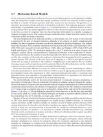
results of the ANN prediction,Q
.
p
ANN
, plotted against the actual measurement, Q
.
e
. The 45° line that is shown is
an exact prediction; the dotted lines represent errors of Ϯ10%. Figure 16.3 also shows the prediction of a
power-law correlation for the same data, Q
.
p
cor
[Zhao, 1995]. The ANN does a better job than the correlation.
16.2.6.2 Thermal Neurocontrol
The same heat exchanger was used to develop the neurocontrol methodology. Dynamic data were obtained
by varying the water inlet temperatures by changing the heater settings while keeping the other variables

constant. Training data were obtained from experiments in which the water inlet temperature was varied
in small increments of 5.56°C from 32.2°C up to 65.6°C. Díaz et al. (2001a) provides further details.
A nonlinear system may be controlled in many different ways. The method chosen for neurocontrol testing
is shown in Figure 16.4.An inverse-ANN controller, C,controls the heat exchanger, while a forward ANN,
M, models the plant, P.The controller is trained as a dynamic ANN. The desired control objective was to
keep the outlet air temperature T
a
out
constant.
In the first test, the system was subjected to a step change in the set temperature. The system was stabilized
around T
a
out
ϭ 32°C, after which the set temperature was suddenly changed to 36°C. Figure 16.5 shows
how the neurocontroller behaved as compared to conventional PID (proportional–integral–derivative)
and PI (proportional–integral) controllers. All the controllers work properly, but the neurocontroller has
Soft Computing in Control 16-7
0 1000 2000 3000 4000 5000 6000 7000 8000 9000
0
1000
2000
3000
4000
5000
6000
7000
8000
9000
10000
Q

e
(W)
Q
p
ANN Q
p
cor (W)
FIGURE 16.3 Predictions of 4–5–5–1 neural network (ϩ) and correlation (᭺).
© 2006 by Taylor & Francis Group, LLC
fewer oscillations. In a second test, we looked at the disturbance rejection ability of the controller. At
steady operation, the water flow is completely shut down for a short interval between t ϭ 40s and t ϭ 70 s.
Figure 16.6 shows how the system variables respond to PID and neurocontrol during and after the dis-
turbance pulse. In the neurocontroller, oscillations are quickly damped out.
The procedure previously outlined in which the ANN simulates the plant to be controlled is fairly
straightforward. Other special aspects should be examined further.
16.2.6.2.1 Stabilization of Feedback Loop
(See [Díaz et al., 2001b].) The static ANN, once incorporated into the feedback loop, may lead to a
dynamical system that is unstable. In order to avoid this possibility, the ANN has to be trained not only
to make accurate predictions but also togivedynamical stability to the loop. Because the weights are not
unique, it is possible to come up with an algorithm that does both. The stabilization algorithm was
designed and tested on the heat exchanger facility. Figure 16.7 shows the behavior of two controllers C
1
and C
2
,where the former is a stable controller and the latter is unstable. In each case, the air flow rate is
being controlled, and the air outlet temperature is shown as a function of time. The stable controller
works well, while in the unstable case the air flow rate is increased as far as possible without achieving the
desired result.
16.2.6.2.2 Adaptive Neurocontrol
(See [Díaz et al., 2001c].) The major advantage of neurocontrollers is that they can be adaptive. The ANN

can go through a process of retraining if its predictions are not accurate due to change in system charac-
teristics.The adaptive controller is tested in two different ways. The first is a disturbance on the water side,
shown in Figure 16.8; v
a
in the figure is the air velocity. Initially, the neurocontroller keeps the system close
to T
a
out
ϭ 34°C. From t ϭ 100 stot ϭ 130s, the water is shut off. The neurocontroller tries to control
until t ϭ 110 s, at which point it hands off to a backup PID controller while it adapts to the new circum-
stances. Then, once it is able to make reasonable predictions, it resumes control at t ϭ 170 s. The second test
isasudden reduction of inlet area of the wind tunnel test facility, shown in Figure 16.9. The controller
keeps T
a
out
at 34°C, and then half of the inlet is suddenly blocked at t ϭ 150 s. The neurocontroller adapts
until it learns the behavior of the new system, and finally at t ϭ 240 s it resumes control of the system.
16-8 MEMS: Introduction and Fundamentals
P
C
M
–
–
+
+
+
+
+
F
–

I
FIGURE 16.4 Closed-loop neurocontrol (P ϭ plant, M ϭ ANN model of plant, C ϭ neurocontroller, F ϭ filter,
I ϭ integral controller).
© 2006 by Taylor & Francis Group, LLC
16.2.6.2.3 Optimal Con trol
For systems where there is more than one variable to be controlled, it is often required that they be con-
trolled under an optimizing constraint. For thermal systems, for example, it may be possible to require
that the system use the least energy at the new setpoint. Figure 16.10 shows the neurocontroller being
used in this mode with the water and air flow rates being the control variables. In this case, the ANN has
been provided information about the energy consumption of the following components of the facility: the
hydraulic pump, the fan, and the electric heater. We first let the controller stabilize T
a
out
at 34°C. Around
t ϭ 130 s, the energy minimization routine turns on, and the controller adjusts both the water and air
flow rates to minimize energy usage while keeping T
a
out
roughly at its set value.
Soft Computing in Control 16-9
36.4
36.2
36
35.8
35.6
35.2
100 120 140 160 180 200 220 240 260 280 300
t [s]
T
out

[°C]
ANN
PID
PI
36.5
36
35.5
35
34.5
34
31.5
32
32.5
33
33.5
0 50 100 150 200 250 300 350
t [s]
T
out
[°C]
ANN
PID
PI
a
FIGURE 16.5 Response to change in set point.
© 2006 by Taylor & Francis Group, LLC
16-10 MEMS: Introduction and Fundamentals
0 50 100 150 200 250 300 350 400
0
200

200
300
T
a
out
(°C)
t (s)
0 50 100 150 200 250 300 350 400
t (s)
0 50 100 150 200 250 300 350 400
t (s)
34.5
35
35.5
36
36.5
0.1
0.2
0.3
0.4
0.5
m
a
(kg/s)
•
m
w
(kg/s)
•
(a)

(b)
(c)
FIGURE 16.6 Disturbance rejection (continuous line is neural network, broken line is PID).
500 100 150 200 250 300 350 400
30
30.5
31
31.5
32
32.5
33
33.5
34
34.5
35
T (°C)
air
out
C
C
1
2
t [s]
FIGURE 16.7 Performance of stable and unstable neurocontrollers.
© 2006 by Taylor & Francis Group, LLC
Soft Computing in Control 16-11
0 50 100 150 200 250 300 350 400 450 500
0 50 100 150 200 250 300 350 400 450 500
33
33.5

34
34.5
35
0.5
1
1.5
2
2.5
3
0 50 100 150 200 250 300 350 400 450 500
40
42
44
46
48
50
T
w
out
(°C) T
a
out
(°C)
v
a
(m/s)
t (s)
t (s)
t (s)
FIGURE 16.8 Response of adaptive neurocontroller to pulsed stoppage in water flow.

0 50 100 150 200 250 300 350
0 50 100 150 200 250 300 350
33
33.5
34
34.5
35
35.5
1
1.5
2
2.5
3
3.5
4
4.5
T
a
out
(°C)
v
a
(m/s)
t (s)
t (s)
FIGURE 16.9 Response of adaptive neurocontroller to sudden change in wind-tunnel inlet area.
© 2006 by Taylor & Francis Group, LLC