The MEMS Handbook MEMS Applications (2nd Ed) - M. Gad el Hak Episode 1 Part 3 pot

3-2 MEMS: Applications
devices in catheters that can aid procedures such as angioplasty.Many industrial applications exist that relate
to monitoring manufacturing processes. In the semiconductor sector, for example, process steps such as
plasma etching or deposition and chemical vapor deposition are very sensitive to operating pressures.
In the long history of using micromachining technology for pressure sensors, device designs have evolved
as the technology has progressed, allowing pressure sensors to serve as technology demonstration vehi-
cles [Wise, 1994]. A number of sensing approaches that offer different relative merits have evolved, and
there has been a steady march toward improving performance parameters such as sensitivity, resolution,
and dynamic range. Although multiple options exist, silicon has been a popular choice for the structural
material of micromachined pressure sensors partly because its material properties are adequate, and there
is significant manufacturing capacity and know-how that can be borrowed from the integrated circuit
industry. The primary focus in this chapter is on schemes that use silicon as the structural material. The
chapter is divided into six sections. The first section introduces structural and performance concepts that
are common to a number of micromachined pressure sensors. The second and third sections focus in some
detail on piezoresistive and capacitive pick-off schemes for detecting pressure. These two schemes form
the basis of the vast majority of micromachined pressure sensors available commercially and studied by
the MEMS research community. Fabrication, packaging, and calibration issues related to these devices are
also addressed in these sections. The fourth section describes servo-controlled pressure sensors, which
represent an emerging theme in research publications. The fifth section surveys alternative approaches
and transduction schemes that may be suitable for selected applications. It includes a few schemes that
have been explored with non-micromachined apparatus, but may be suitable for miniaturization in the
future. The sixth section concludes the chapter.
3.2 Device Structure and Performance Measures
The essential feature of most micromachined pressure sensors is an edge-supported diaphragm that
deflects in response to a transverse pressure differential across it. This deformation is typically detected by
measuring the stresses in the diaphragm, or by measuring the displacement of the diaphragm. An example
of the former approach is the piezoresistive pick-off, in which resistors are formed at specific locations of
the diaphragm to measure the stress. An example of the latter approach is the capacitive pick-off, in which
an electrode is located on a substrate some distance below the diaphragm to capacitively measure its dis-
placement. The choice of silicon as a structural material is amenable to both approaches because it has a
relatively large piezoresistive coefficient and because it can serve as an electrode for a capacitor as well.

3.2.1 Pressure on a Diaphragm
The deflection of a diaphragm and the stresses associated with it can be calculated analytically in many
cases. It is generally worthwhile to make some simplifying assumptions regarding the dimensions and
boundary conditions. One approach is to assume that the edges are simply supported. This is a reason-
able approximation if the thickness of the diaphragm, h, is much smaller than its radius, a. This condi-
tion prevents transverse displacement of the neutral surface at the perimeter, while allowing rotational
and longitudinal displacement. Mathematically, it permits the second derivative of the deflection to be
zero at the edge of the diaphragm. However, the preferred assumption is that the edges of the diaphragm
are rigidly affixed (built-in) to the support around its perimeter. Under this assumption the stress on the
lower surface of a circular diaphragm can be expressed in polar coordinates by the equations:
σ
r
ϭ [a
2
(1 ϩ v) Ϫ r
2
(3 ϩ v)] (3.1)
σ
t
ϭ [a
2
(1 ϩ v) Ϫ r
2
(1 ϩ 3v)] (3.2)
3 и ∆P
ᎏ
8h
2
3 и ∆P
ᎏ

8h
2
© 2006 by Taylor & Francis Group, LLC
where the former denotes the radial component and the latter the tangential component, a and h are the
radius and thickness of the diaphragm, r is the radial co-ordinate, ∆P is the pressure applied to the upper
surface of the diaphragm, and
ν
is Poisson’s ratio (Figure 3.1) [Timoshenko and Woinowsky-Krieger,
1959; Samaun et al., 1973; Middleoek and Audet, 1994]. In the (100) plane of silicon, Poisson’s ratio
shows four-fold symmetry, and varies from 0.066 in the [011] direction to 0.28 in the [001] direction
[Evans and Evans, 1965’ Madou, 1997]. These equations indicate that both components of stress vary
from the same tensile maximum at the center of the diaphragm to different compressive maxima at its
periphery. Both components are zero at separate values of r between zero and a. In general, piezoresistors
located at the points of highest compressive and tensile stress will provide the largest responses. The
deflection of a circular diaphragm under the stated assumptions is given by:
d ϭ
(3.3)
where E is the Young’s modulus of the structural material. This is valid for a thin diaphragm with simply
supported edges, assuming a small defection.
Like Poisson’s ratio, the Young’s modulus for silicon shows four-fold symmetry in the (100) plane, vary-
ing from 168 GPa in the [011] direction to 129.5 GPa in the [100] direction [Greenwood, 1988; Madou,
1997]. When polycrystalline silicon (polysilicon) is used as the structural material, the composite effect
of grains of varying size and crystalline orientation can cause substantial variations. It is important to note
that additional variations in mechanical properties may arise from crystal defects caused by doping and
other disruptions of the lattice. Equation 3.3 indicates that the maximum deflection of a diaphragm is at
its center, which comes as no surprise. More importantly, it is dependent on the radius to the fourth power,
and on the thickness to the third power, making it extremely sensitive to inadvertent variations in these
dimensions. This can be of some consequence in controlling the sensitivity of capacitive pressure sensors.
3.2.2 Square Diaphragm
For pressure sensors that are micromachined from bulk Si, it is common to use anisotropic wet etchants

that are selective to crystallographic planes, which results in square diaphragms. The deflection of a
square diaphragm with built-in edges can be related to applied pressure by the following expression:
∆P ϭ
΄
4.20 ϩ 1.58
΅
(3.4)
where a is half the length of one side of the diaphragm [Chau and Wise, 1987]. This equation provides a
reasonable approximation of the maximum deflection over a wide range of pressures, and is not limited
to small deflections. The first term within this equation dominates for small deflections, for which w
c
Ͻ h,
whereas the second term dominates for large deflections. For very large deflections, it approaches the
deflection predicted for flexible membranes with a 13% error.
3.2.3 Residual Stress
It should be noted that the analysis presented above assumes that the residual stress in the diaphragm is
negligibly small. Although mathematically convenient, this is often not the case. In reality, a tensile stress
w
3
c
ᎏ
h
3
w
c
ᎏ
h
Eh
4
ᎏᎏ

(1 Ϫ
v
2
)a
4
3 и ∆P(1 Ϫ
ν
2
)(a
2
Ϫ r
2
)
2
ᎏᎏᎏ
16Eh
3
Micromachined Pressure Sensors: Devices, Interface Circuits, and Performance Limits 3-3
∆P
a
r
d
FIGURE 3.1 Deflection of a diaphragm under applied pressure.
© 2006 by Taylor & Francis Group, LLC
of 5–50MPa is not uncommon. This may significantly reduce the sensitivity of certain designs, particu-
larly if the diaphragm is very thin. Following the treatment in Chau and Wise (1987) for a small deflection
in a circular diaphragm with built-in edges, the governing differential equation is:
ϩ Ϫ
΂
ϩ

΃
φ
ϭ Ϫ
(3.5)
where
σ
i
is the intrinsic or residual stress in the undeflected diaphragm, D ϭ Eh
3
/[12(1 Ϫ
ν
2
)], and
φ
ϭϪdw/dr is the slope of the deformed diaphragm. The solution this differential equation provides w:
w
ϭ
∆P и a
4
΄
I
0
΂΃
Ϫ I
0
(k)
΅
∆P и a
2
(a

2
Ϫ r
2
)
2k
3
I
1
(k)D
ϩ
4k
2
D
(3.6)
in tension, and
w
ϭ
∆P и a
4
΄
J
0
΂΃
Ϫ J
0
(k)
΅
∆P
и
a

2
(a
2
Ϫ r
2
)
2k
3
J
1
(k)D
ϩ
4k
2
D
(3.7)
in compression. In these expressions, J
n
and I
n
are the Bessel function and the modified Bessel function
of the first kind of order n,respectively. The term k is given by:
k
2
ϭ ϭ
(3.8)
The maximum deflection (at the center of the diaphragm), normalized to the deflection in the absence
of residual stress, is provided by:
wЈ
c

ϭ
(3.9)
in tension, and
wЈ
c
ϭ
(3.10)
in compression. It is instructive to evaluate the dependence of this normalized deflection to the dimen-
sionless intrinsic stress, which is defined by:
σ
Ј
i
ϭ
(3.11)
As shown in Figure 3.2,residual stress can have a tremendous impact on deflection: atensile dimension-
less stress of 1.3 diminishes the center deflection by 50%. For tensile (positive) values of
σ
Ј
i
exceeding 10,
the center deflection (not normalized) can be approximated as for a membrane:
w
c
ϭ
(3.12)
Returning to Figure 3.2, it is evident that the deflection can be increased by compressive stress. However,
even relatively small values of compressive stress can result in buckling, so it is not generally perceived as
a feature that can be reliably exploited.
3.2.4 Composite Diaphragms
In micromachined pressure sensors, it is often the case that the diaphragm is fabricated not from a single

material but from composite layers. For example, a silicon membrane can be covered by a layer of SiO
2
∆P и a
2
ᎏ
4
σ
i
h
(1 Ϫ
ν
2
)
σ
i
a
2
ᎏᎏ
Eh
2
16[2 Ϫ 2J
0
(k) ϩ kJ
1
(k)]
ᎏᎏᎏ
k
3
J
1

(k)
16[2 Ϫ 2I
0
(k) ϩ kI
1
(k)]
ᎏᎏᎏ
k
3
I
1
(k)
12(1 Ϫ v
2
)
σ
i
a
2
ᎏᎏ
Eh
2

σ
i
a
2
h
ᎏ
D

kr
ᎏ
a
kr
ᎏ
a
∆P и r
ᎏ
2D
1
ᎏ
r
2
σ
i
h
ᎏ
D
d
φ
ᎏ
dr
1
ᎏ
r
d
2
φ
ᎏ
dr

2
3-4 MEMS: Applications
© 2006 by Taylor & Francis Group, LLC
or Si
x
N
y
for electrical isolation. In general, these films can be of comparable thickness, and have values of
Young’s modulus and residual stress that are significantly different. The residual stress of a composite
membrane is given by:
σ
c
t
c
ϭ
Α
m
σ
m
t
m
(3.13)
where
σ
c
and t
c
denote the composite stress and thickness, respectively, while
σ
m

and t
m
denote the stress
and thickness of individual films. Furthermore, if the Poisson’s ratio of all the layers in the membrane is
comparable, the following approximation may be used for the Young’s modulus:
E
c
t
c
ϭ
Α
m
E
m
t
m
(3.14)
where the suffixes have the same meaning as in the preceding equation.
3.2.5 Categories and Units
Pressure sensors are typically divided into three categories: absolute, gauge, and differential (relative)
pressure sensors. Absolute pressure sensors provide an output referenced to vacuum, and often accomplish
this by vacuum sealing a cavity underneath the diaphragm. The output of a gauge pressure sensor is ref-
erenced to atmospheric pressure. A differential pressure sensor compares the pressure at two input ports,
which typically transfer the pressure to different sides of the diaphragm.
A number of different units are used to denote pressure, which can lead to some confusion when com-
paring performance ratings. One atmosphere of pressure is equivalent to 14.696 pounds per square inch (psi),
101.33 kPa, 1.0133 bar (or centimeters of H
2
0 at 4°C), and 760 Torr (or millimeters of Hg at 0°C).
3.2.6 Performance Criteria

The performance criteria of primary interest in pressure sensors are sensitivity, dynamic range, full-scale
output, linearity, and the temperature coefficients of sensitivity and offset. These characteristics depend
Micromachined Pressure Sensors: Devices, Interface Circuits, and Performance Limits 3-5
0.1
0.01
0.1
1
10
100
1 10 100
Center deflection
(Compression)
Center deflection
(Tension)
Pressure sensitivity
(Compression)
Pressure sensitivity
(Tension)
Dimensionless stress (1−v
2
)

l
a
2
/Eh
2
Normalized pressure sensitivity
and diaphragm center deflection
FIGURE 3.2 Normalized deflection of a circular diaphragm as a function of dimensionless stress. (Reprinted with

permission from Chau, H., and Wise, K. [1987a] “Noise Due to Brownian Motion in Ultrasensitive Solid-State
Pressure Sensors,” IEEE Transactions on Electron Devices 34, pp. 859–865.)
© 2006 by Taylor & Francis Group, LLC
on the device geometry, the mechanical and thermal properties of the structural and packaging materi-
als, and selected sensing scheme. Sensitivity is defined as a normalized signal change per unit pressure
change to reference signal:
S ϭ (3.15)
where
θ
is output signal and ∂
θ
is the change in this pressure due to the applied pressure ∂P. Dynamic
range is the pressure range over which the sensor can provide a meaningful output. It may be limited by
the saturation of the transduced output signal such as the piezoresistance or capacitance. It also may be
limited by yield and failure of the pressure diaphragm. The full-scale output (FSO) of a pressure sensor
is simply the algebraic difference in the end points of the output. Linearity refers to the proximity of the
device response to a specified straight line. It is the maximum separation between the output and the line,
expressed as a percentage of FSO. Generally, capacitive pressure sensors provide highly non-linear outputs,
and piezoresistive pressure sensors provide fairly linear output.
The temperature sensitivity of a pressure sensor is an important performance metric. The definition
of temperature coefficient of sensitivity (TCS) is:
TCS ϭ (3.16)
where S is sensitivity. Another important parameter is the temperature coefficient of offset (TCO). The
offset of a pressure sensor is the value of the output signal at a reference pressure, such as when ∆P ϭ 0.
Consequently, the TCO is:
TCO ϭ (3.17)
where
θ
0
is offset, and T is temperature. Thermal stresses caused by differences in expansion coefficients

between the diaphragm and the substrate or packaging materials are some of the many possible contributors
to these temperature coefficients.
3.3 Piezoresistive Pressure Sensors
The majority of commercially available micromachined pressure sensors are bulk micromachined piezore-
sistive devices. These devices are etched from single crystal silicon wafers, which have relatively well-
controlled mechanical properties. The diaphragm can be formed by etching the back of a Ͻ100Ͼ oriented
Si wafer with an anisotropic wet etchant such as potassium hydroxide (KOH). An electrochemical etch-
stop, dopant-selective etch-stop, or a layer of buried oxide can be used to terminate the etch and control
the thickness of the unetched diaphragm. This diaphragm is supported at its perimeter by a portion of
the wafer that was not exposed to the etchant and remains at full thickness (Figure 3.1). The piezoresistors
are fashioned by selectively doping portions of the diaphragm to form junction-isolated resistors. Although
this form of isolation permits significant leakage current at elevated temperatures and the resistors present
sheet resistance per unit length that depends on the local bias across the isolation diode, it allows the
designer to exploit the substantial piezoresistive coefficient of silicon and locate the resistors at the points
of maximum stress on the diaphragm.
Surface micromachined piezoresistive pressure sensors have also been reported. Sugiyama et al. (1991)
used silicon nitride as the structural material for the diaphragm. Polycrystalline silicon (polysilicon) was
used both as a sacrificial material and to form the piezoresistors. This approach permits the fabrication
of small devices with high packing density. However, the maximum deflection of the diaphragm is lim-
ited to the thickness of the sacrificial layer, and can constrain the dynamic range. In Guckel et al. (1986),
(reprinted in Microsensors (1990)) polysilicon was used to form both the diaphragm and the piezoresistors.
∂
θ
0
ᎏ
∂T
1
ᎏ
θ
0

∂S
ᎏ
∂T
1
ᎏ
S
∂
θ
ᎏ
∂P
1
ᎏ
θ
3-6 MEMS: Applications
© 2006 by Taylor & Francis Group, LLC
3.3.1 Design Equations
In an anisotropic material such as single crystal silicon, resistivity is defined by a tensor that relates the
three directional components of the electric field to the three directional components of current flow. In
general, the tensor has nine elements expressed in a 3 ϫ 3 matrix, but they reduce to six independent val-
ues from symmetry considerations:
΄΅
ϭ
΄ ΅΄΅
(3.18)
where
ε
i
and j
i
represent electric field and current density components, and

ρ
i
represent resistivity com-
ponents. Following the treatment in Kloeck and de Rooij (1994) and Middleoek and Audet (1994), if the
Cartesian axes are aligned to the Ͻ100Ͼ axes in a cubic crystal structure such as silicon,
ρ
1
,
ρ
2
, and
ρ
3
will
be equal because they all represent resistance along the Ͻ100Ͼ axes, and are denoted by
ρ
. The remain-
ing components of the resistivity matrix, which represent cross-axis resistivities, will be zero because
unstressed silicon is electrically isotropic. When stress is applied to silicon, the components in the resis-
tivity matrix change. The change in each of the six independent components, ∆
ρ
i
, will be related to all the
stress components. The stress can always be decomposed into three normal components (
σ
i
), and three
shear components (
τ
i

), as shown in Figure 3.3. The change in the six components of the resistivity matrix
(expressed as a fraction of the unstressed resistivity
ρ
) can then be related to the six stress components by
a 36-element tensor. However, due to symmetry conditions, this tensor is populated by only three non-
zero components, as shown:
΄ ΅
ϭ
΄ ΅
ϩ
΄ ΅
;
΄ ΅
ϭ
΄ ΅΄ ΅
(3.19)
σ
1
σ
2
σ
3
τ
1
τ
2
τ
3
0
0

0
0
0
π
44
0
0
0
0
π
44
0
0
0
0
π
44
0
0
π
12
π
12
π
11
0
0
0
π
12

π
11
π
12
0
0
0
π
11
π
12
π
12
0
0
0
∆
ρ
1
∆
ρ
2
∆
ρ
3
∆
ρ
4
∆
ρ

5
∆
ρ
6
1
ᎏ
ρ
∆
ρ
1
∆
ρ
2
∆
ρ
3
∆
ρ
4
∆
ρ
5
∆
ρ
6
ρ
ρ
ρ
0
0

0
ρ
1
ρ
2
ρ
3
ρ
4
ρ
5
ρ
6
j
1
j
2
j
3
ρ
5
ρ
4
ρ
3
ρ
6
ρ
2
ρ

4
ρ
1
ρ
6
ρ
5
ε
1
ε
2
ε
3
Micromachined Pressure Sensors: Devices, Interface Circuits, and Performance Limits 3-7
X
Y
Z

1

3

2

2

3

3


1

1

2
FIGURE 3.3 Definition of normal and shear stresses.
© 2006 by Taylor & Francis Group, LLC
where the
π
ij
coefficients, which have units of Pa
Ϫ1
,may be either positive or negative, and are sensitive
to doping type, doping level, and operating temperature. It is evident that
π
11
relates the resistivity in any
direction to stress in the same direction, whereas
π
12
and
π
44
are cross-terms.
Equation 3.19 was derived in the context of acoordinate system aligned to the Ͻ100Ͼ axes, and is not
always convenient to apply. A preferred representation is to express the fractional change in an arbitrar-
ily oriented diffused resistor by:
ϭ
π
l

σ
l
ϩ
π
t
σ
t
(3.20)
where
π
l
and
σ
l
are the piezoresistive coefficient and stress parallel to the direction of current flow in the
resistor (i.e., parallel to its length), and
π
t
and
σ
t
are the values in the transverse direction. The piezore-
sistive coefficients referenced to the direction of the resistor may be obtained from those referenced to
the Ͻ100Ͼ axes in Equation 3.19 by using a transformation of the coordinate system. It can then be
stated that:
π
l
ϭ
π
11

ϩ 2(
π
44
ϩ
π
12
Ϫ
π
11
)(l
2
1
m
2
1
ϩ l
2
1
n
2
1
ϩ n
2
1
m
2
1
) (3.21)
π
t

ϭ
π
12
Ϫ (
π
44
ϩ
π
12
Ϫ
π
11
)(l
2
1
l
2
2
ϩ m
2
1
m
2
2
ϩ n
2
1
n
2
2

) (3.22)
where l
1
,m
1
, and n
1
are the direction cosines (with respect to the crystallographic axes) of a unit length
vector, which is parallel to the current flow in the resistor whereas l
2
,m
2
, and n
2
are those for a unit length
vector perpendicular to the resistor. Thus, l
i
2
ϩ m
i
2
ϩ n
i
2
ϭ 1. As an example, for the Ͻ111Ͼ direction, in
which projections to all three crystallographic axes are equal, l
i
2
ϭ m
i

2
ϭ n
i
2
ϭ 1/3.
A sample set of piezoresistive coefficients for Si is listed in Table 3.1.It is evident that
π
44
dominates for
p-type Si, with a value that is more than 20 times larger than the other coefficients. By using the domi-
nant coefficient and neglecting the smaller ones, Equations 3.21 and 3.22 can be further simplified. It
should be noted, however, that the piezoresistive coefficient can vary significantly with doping level and
operating temperature of the resistor. A convenient way in whichtorepresent the changes is to normal-
ize the piezoresistive coefficient to a value obtained at room temperature for weakly doped silicon
[Kanda, 1982]:
π
(N,T) ϭ P(N,T)
π
ref
.
(3.23)
Figure 3.4 shows the variation of parameter P for p-type and n-type Si, as N, the doping concentration,
and T, the temperature, are varied.
Figure 3.5 plots the longitudinal and transverse piezoresistive coefficients for resistor orientations on
the surface of a (100) silicon wafer. Note that each figure is split into two halves, showing
π
l
and
π
t

simul-
taneously for p-type Si in one case and n-type Si in the other case. Each curve would be reflected in the
horizontal axis if drawn individually. Also note that for p-type Si, both
π
l
and
π
t
peak along Ͻ110Ͼ ,
whereas for n-type Si, they peak along Ͻ100Ͼ .Since anisotropic wet etchants make trenches aligned
to Ͻ110Ͼ on these wafer surfaces, p-type piezoresistors, which can be conveniently aligned parallel or
perpendicular to the etched pits, are favored.
Consider two p-type resistors aligned to the Ͻ110Ͼ axes and near the perimeter of a circular
diaphragm on a silicon wafer: assume that one resistor is parallel to the radius of the diaphragm, whereas
the other is perpendicular to it. Using the equations presented previously, it can be shown that as pres-
sure is applied, the fractional change in these resistors is equal and opposite:
΂ ΃
ra
ϭ Ϫ
΂ ΃
ta
ϭϪ
∆P и
(3.24)
where the subscripts denote radial and tangentially oriented resistors. The complementary change in
these resistors is well-suited to a bridge-type arrangement for readout, as shown in Figure 3.6.
3
π
44
a

2
(1 Ϫ v)
ᎏᎏ
8h
2
∆R
ᎏ
R
∆R
ᎏ
R
∆R
ᎏ
R
3-8 MEMS: Applications
© 2006 by Taylor & Francis Group, LLC
(The bridge-type readout arrangement is suitable for square diaphragms as well.) The output voltage in
this case is given by:
∆
∆
V
0
ϭ V
s
(3.25)
∆R
ᎏ
R
Micromachined Pressure Sensors: Devices, Interface Circuits, and Performance Limits 3-9
TABLE 3.1 A Sample of Room Temperature Piezoresistive

Coefficients in Si in 10
Ϫ11
Pa
Ϫ1
. (Reprinted with Permission
from Smith, C.S. [1954] “Piezoresistance Effect in Germanium
and Silicon,” Physical Review 94, pp. 42–49
Resistivity
π
11
π
12
π
44
7.8 ⍀ cm, p-type 6.6 Ϫ1.1 138.1
11.7 ⍀ cm, n-type Ϫ102.2 53.4 Ϫ13.6
0
0
0.5
1.0
1.5
10
16
10
16
10
17
10
18
10

19
10
20
10
17
10
18
10
19
10
20
0.5
1.0
1.5
N (cm
−3
)
N (cm
−3
)
P(N,T)
P(N,T)
p-Si
n-Si
T = −75°C
T = −50°C
T = −25°C
T = 0°C
T = 25°C
T = 50°C

T = 75°C
T = 100°C
T = 150°C
T = 125°C
T = 175°C
T = −75°C
T = −50°C
T = −25°C
T = 0°C
T = 25°C
T = 50°C
T = 75°C
T = 100°C
T = 150°C
T = 125°C
T = 175°C
FIGURE 3.4 Variation of piezoresistive coefficient for n-type and p-type Si. (Reprinted with permission from
Kanda, Y. [1982] “A Graphical Representation of the Piezoresistive Coefficients in Si,” IEEE Transactions on Electron
Devices 29, pp. 64–70.)
© 2006 by Taylor & Francis Group, LLC
3-10 MEMS: Applications
0 0
90
90
100
100
110
110
120
120

130
130
140
140
150
150
160
160
170
170
10
10
20
20
30
30
40
40
50
50
60
60
70
70
80
80
20 30
40 50
60 70 80 90 100 110
20 30 40 50 60 70 80 90 100 110

−110 −100 −90
−80
−70 −60
−50
−40 −30
−110 −100−90 −80 −70 −60 −50 −40 −30
−20
−20
[010]
[110]
[100]
[010]

l

t
0 0
90
90
1
0
0
1
0
0
110
110
120
120
130

130
140
140
150
150
1
6
0
1
6
0
170
170
1
0
1
0
20
20
30
30
40
40
50
50
6
0
6
0
70

70
80
80
20 30
40 50
60 70 80 90 100 110
20 30 40 50 60 70 80 90 100 110
−
110−100 −90
−80
−
70 −60
−50
−40 −30
−110 −90 −80 −70 −60 −50 −40 −30
−20
−
20
[010]
[110]
[100]
[010]
[110]
[110]

l

t
−100
FIGURE 3.5 Longitudinal and transverse piezoresistive coefficients for n-type (upper) and p-type (lower) resistors

on the surface of a (100) Si wafer. (Reprinted with permission from Kanda, Y. [1982] “A Graphical Representation of
the Piezoresistive Coefficients in Si,” IEEE Transactions on Electron Devices 29, pp. 64–70.)
© 2006 by Taylor & Francis Group, LLC
Since the output is proportional to the supply voltage V
s
, the output voltage of piezoresistive pressure sen-
sors is generally presented as a fraction of the supply voltage per unit change in pressure. It is proportional
to a
2
/h
2
, and is typically on the order of 100 ppm/Torr. The maximum fractional change in a piezoresistor
is in the order of 1% to 2%. It is evident from Equations 3.24 and 3.25 that the temperature coefficient of
sensitivity, which is the fractional change in the sensitivity per unit change in temperature, is primarily
governed by the temperature coefficient of
π
44
. A typical value for this is in the range of 1000–5000 ppm/K.
While this is large, its dependence on
π
makes it relatively repeatable and predictable, and permits it to
be compensated.
A valuable feature of the resistor bridge is the relatively low impedance that it presents. This permits the
remainder of the sensing circuit to be located at some distance from the diaphragm, without deleterious
effects from parasitic capacitance that may be incorporated. This stands in contrast to the output from
capacitive pickoff pressure sensors, for which the high output impedance creates significant challenges.
3.3.2 Scaling
The resistors present a scaling limitation for the pressure sensors. As the length of a resistor is decreased,
the resistance decreases and the power consumption rises, which is not favorable.As the width is decreased,
minute variations that may occur because of non-ideal lithography or other processing limitations will

have a more significant impact on the resistance. These issues constrain how small a resistor can be made.
As the size of the diaphragm is reduced, the resistors will span a larger area between its perimeter and the
center. Since the maximum stresses occur at these locations, a resistor that extends between them will be
subject to stress averaging, and the sensitivity of the readout will be compromised. In addition, if the nom-
inal values of the resistors vary, the two legs of the bridge become unbalanced, and the circuit presents a
non-zero signal even when the diaphragm is undeflected. This offset varies with temperature and cannot
be easily compensated because it is in general unsystematic.
3.3.3 Noise
There are three general sources of noise that must be evaluated for piezoresistive pressure sensors, including
mechanical vibration of the diaphragm, electrical noise from the piezoresistors, and electrical noise from
the interface circuit. Thermal energy in the form of Brownian motion of the gas molecules surrounding
the diaphragm causes variations in its deflection that can be treated as though caused by an equivalent
pressure. The treatment in Chau and Wise (1987) and Chau and Wise (1987a) provides a solution for rar-
efied gas environments in which the mean free path between collisions of the gas molecules is much larger
Micromachined Pressure Sensors: Devices, Interface Circuits, and Performance Limits 3-11
R + ∆R
V
0
Tangential
resistor
Radial
resistor
R + ∆R
R − ∆R
R − ∆R
V
s
FIGURE 3.6 Schematic representation of Wheatstone bridge configuration (left) and placement of radial and tan-
gential strain sensors on a circular diaphragm (right).
© 2006 by Taylor & Francis Group, LLC

than the dimensions of the diaphragm. For a circular diaphragm with built-in edges, the noise equivalent
mean square pressure at low frequencies (i.e. in a bandwidth limited by the pressure sensor), is given by:
p
ෆ
2
ෆ
n
ෆ
ϭ
α
Ί
๶
(3.26)
where B is the system bandwidth, T is absolute temperature, k is Boltzmann’s constant, m
1
and m
2
are the
masses of gas molecules, P
1
and P
2
, are the respective pressures on the two sides of the diaphragm, and
α
is 1.7. It is worth noting that this treatment of intrinsic diaphragm noise is for relatively low pressures, at
which the levels gas noise is relatively small. It ignores the thermal vibrations within the structural material
because these are typically even smaller. However, this is not necessarily true in very high vacuum envi-
ronments, which may permit noise from the thermal vibrations of the structural materials to dominate.
At higher pressures, for which viscous damping dominates, the mean square noise pressure on the sur-
face of the diaphragm is given by:

p
ෆ
2
ෆ
n
ෆ
ϭ 4kTR
a
(3.27)
where R
a
is the mechanical resistance (damping) coefficient per unit active area, i.e., R/A, where R is the total
damping coefficient and A is the area of the diaphragm [Gabrielson, 1993]. The term R may also be stated as
m
ω
o
/Q, in which m is the effective mass per unit area of the diaphragm,
ω
o
is the resonant frequency, and
Q is the mechanical quality factor of the diaphragm resonance.
Squeeze film damping between the diaphragm and any opposing surface can be a very significant con-
tributor to sensor noise. Since this is more important in capacitive pressure sensors because of the relatively
small gap between the diaphragm and the sensing counter-electrode, it is discussed in the next section.
In addition, thermally generated acoustic waves also deserve attention at higher pressures. The approx-
imate two-sided power spectrum is given by Chau and Wise (1987):
S
a
(f)
ϭ

(3.28)
where S
a
is the input noise pressure,
ρ
is the density, f is the frequency, and c is the speed of sound in the
fluid surrounding the pressure sensor. This is evidently significant at higher frequencies, and is typically
significant above 10 KHz.
The electrical noise from the piezoresistor, identified above as the second of three components, is also
Brownian in origin. The equivalent noise pressure from this source can be presented as:
p
ෆ
2
ෆ
n
ෆ
ϭ
(3.29)
where V
s
is the voltage of the power supply used for the resistor bridge, and S
p
is the sensitivity of the
piezoresistive pressure sensor [Chau and Wise, 1987]. It was noted following Equation 3.25 that S
p
is pro-
portional to (a
2
/h
2

), which makes this component of mean square noise pressure proportional to (h
4
/a
4
).
In many cases, the dominant noise source is not the sensor itself but the interface circuit. If ∆V
min
rep-
resents the minimum voltage difference that can be resolved by the interface circuit, then the pressure res-
olution limit becomes:
Γ
ckt
ϭ
(3.30)
which is proportional to (h
2
/a
2
) [Chau and Wise, 1987].
In comparing the noise sources identified for piezoresistive pressure sensors, the following examples are
useful [Chau and Wise, 1987]. For a small device with diaphragm length of 100µm and thickness 1 µm,
the Brownian noise in a 100 Hz bandwidth and 760 Torr on both sides of the diaphragm is Ͻ10
Ϫ5
Torr.
∆V
min
ᎏ
(V
s
S

p
)
4kTRB
ᎏ
(V
s
S
p
)
2
2
π
kT
ρ
f
2
ᎏ
c
(
͙m
ෆ
1
ෆ
P
1
ϩ
͙m
ෆ
2
ෆ

P
2
)B
ᎏᎏᎏ
a
2
32kT
ᎏ
π
3-12 MEMS: Applications
© 2006 by Taylor & Francis Group, LLC
The piezoresistor noise, assuming a 2 kΩ bridge resistance and a 5V supply, is about 0.11 mTorr, and the cir-
cuit noise is 1.5 mTorr assuming that the minimum resolvable voltage is 0.5 µV. I n c o n t r ast, a 1 mm long
diaphragm of 1 µm thickness has 4 ϫ 10
Ϫ6
mTorr Brownian noise, 1.1 ϫ 10
Ϫ3
mTorr piezoresistor noise,
and 9.5 ϫ 10
Ϫ
3
mTorr circuit noise. In all of these calculations, the component identified in Equation
3.27 is ignored.
3.3.4 Interface Circuits for Piezoresistive Pressure Sensors
An instrumentation amplifier is a natural choice for interfacing with a piezoresistive full-bridge. In such
an arrangement, the differential output labeled V
0
in Figure 3.6 would be connected to the two input ter-
minals labeled
ν

1
and
ν
2
in Figure 3.7. The instrumentation amplifier has two stages [Sedra and Smith,
1998]. In the first stage, which is formed by operational amplifiers A
1
and A
2
, the virtual short circuits
between the two inputs of each of these amplifiers force the current flow in the resistor R
1
to be (
ν
1
Ϫ
ν
2
)/R
1
.
Since the input impedance of the op amps is large, the same current also flows through the two resistors
labeled R
2
, causing the voltage difference between the outputs of A
1
and A
2
to be:
v

o1
Ϫ
v
o2
ϭ
΂
1
ϩ
΃
(
v
1
Ϫ
v
2
)
(3.31)
Thus, the gain provided by this first stage can be changed by varying the value of R
1
.The second stage is
simply a difference amplifier formed by op amp A
3
and the surrounding resistors. This causes the output
voltage to be:
v
0
ϭ
΂
Ϫ
΃

(v
o1
Ϫ v
o2
)
(3.32)
A separate gain stage can be added to the circuit past the instrumentation amplifier. This may also be used
to subtract the temperature dependence of the signal that can be generated as reference voltage from the
top of a current-driven bridge.
Spencer et al. (1985) described another type of circuit that can be used to read out a resistor bridge, which
is a voltage controlled duty-cycle oscillator (VCDCO). As shown in Figure 3.8, this circuit incorporates a
cross-coupled multi-vibrator formed essentially by Q
1
, Q
2
, and the surrounding passive elements. The
input voltage, v
IN
, which is provided by the output of the resistor bridge, determines the ratio of the cur-
rents in the emitter-coupled stage formed by Q
3
and Q
4
:
ϭ
exp
΂ ΃
(3.33)
qν
IN

ᎏ
kT
I
C3
ᎏ
I
C4
R
4
ᎏ
R
3
2R
2
ᎏ
R
1
Micromachined Pressure Sensors: Devices, Interface Circuits, and Performance Limits 3-13
R
1
R
3
R
3
R
2
R
2
R
4

R
4
A
2
−
+
A
3
−
−
+
+
A
1
+
−
υ
o
v
o2
v
o1
v
1
v
2
FIGURE 3.7 Schematic of an instrumentation amplifier used to read out a resistor bridge circuit (Reprinted with per-
mission from Sedra, A.S., and Smith, K.C. [1998] Microelectronic Circuits, 4th ed., Oxford University Press, Oxford.)
© 2006 by Taylor & Francis Group, LLC
The output of the circuit, as illustrated in Figure 3.8, is a square wave, which shows a dependence on the

input voltage in both the duty cycle and period. To understand the operation of the circuit and obtain a sim-
ple quantitative model for its behavior, one may begin with the assumption that the output has just switched
low, causing Q
1
to turn off. In terms of the timing diagram, this is the beginning of t
2
. The entire tail current
I
EE
, then, is provided by Q
2
, and neglects the base current of Q
2
, v
z
Ϸ V
CC
, which causes v
y
to eventually settle
at approximately V
CC
Ϫ 0.7 V; i.e., below v
z
by the drop across the base-to-emitter diode of Q
2
. This condition
also sets v
OUT
at V

CC
Ϫ R.I
EE
. With Q
1
turned off, Q
3
continues to extract I
C3
from C until v
x
drops below v
OUT
by 0.7V, which causes Q
1
to turn on, drop v
z
, and thereby turn off Q
2
. This in turn causes v
OUT
to rise, ending
the time period t
2
. Thus, at the end of t
2
, the voltage across C, v
x
– v
y

Ϸ (V
CC
Ϫ R.I
EE
Ϫ 0.7) –
(V
CC
Ϫ 0.7 V) ϭ ϪR.I
EE
. Similarly, at the end of t
1
, this is ϩR.I
EE
. The change in voltage across C, in either
t
1
or t
2
, is therefore 2R.I
EE
. The resulting change in charge must be balanced by the current flow in the given
time interval, thus:
t
1
Ϸ ; t
2
Ϸ (3.34)
Since I
C3
ϩ I

C4
ϭ I
EE
, using equations (3.33) and (3.34), it can be shown that:
t
1
Ϸ 2RC
Ά
1 ϩ exp
΂ ΃·
, and (3.35)
qv
IN
ᎏ
kT
2RCI
EE
ᎏ
I
C3
2RCI
EE
ᎏ
I
C4
3-14 MEMS: Applications
V
cc
Q
1

Q
3
Q
4
I
EE
Q
2
V
OH
V
OL
t
1
t
2
t
V
z
V
x
V
y
R
R
C
+
−
υ
in

υ
out
FIGURE 3.8 Schematic of a duty cycle oscillator used to read out resistance-based sensors (Reprinted with permis-
sion from Spencer, R.R., Fleischer, B.M., Barth, P.W., and Angell, J.B. (1985) “The Voltage Controlled Duty-Cycle
Oscillator: Basis for a New A-to-D Conversion Technique,” Rec. of the Third International Conference On Solid-State
Sensors and Actuators, pp. 49–52.)
© 2006 by Taylor & Francis Group, LLC
v
IN
ϭ
΂΃
ln
΂ ΃
(3.36)
This equation can be used to determine the input voltage from a measurement of t
1
and t
2
.An important
result is that any ratio that involves t
1
and t
2
is independent of all circuit variables; drifts in their values
over time will not affect the accuracy and resolution of the readout. An exception to this immunity is the
input offset of Q
3
and Q
4
,which can affect the signal. It is also worth noting that the output is pseudo-

digital, in that it is discretized in voltage, although not in time. However, the time durations can be easily
clocked, making the circuit conducive to analog-to-digital conversion of the output signal.
3.3.5 Calibration and Compensation
Regardless of the choice of interface circuit, it is generally necessary to calibrate the overall output. For
the circuit in Figure 3.8, the input voltage can be expressed as the sum of two components: one which
carries the pressure information as represented in Equation 3.25, and a non-ideal offset term which was
previously ignored:
v
IN
ϭ
΂΃
V
s
ϩ v
OFF
ϭ ∆P и SV
s
ϩ v
OFF
(3.37)
where S is the sensitivity of the pressure sensor, V
s
is the supply to the piezoresistor bridge, and v
OFF
is the
offset voltage presented not only by the resistor bridge, but also incorporates the offset due to mismatch
in Q
3
and Q
4

in Figure 3.8. The sensitivity and offset voltage are both functions of temperature, with lin-
earized dependences described in Equations 3.16 and 3.17 as TCS and TCO, respectively. Using (3.26) and
(3.37), it can be stated that the pressure across the diaphragm is given by:
∆P ϭ
΂ ΃
ln
΂΃
Ϫ
΂ ΃
(3.38)
Use of this equation requires the determination of S, v
OFF
, and their temperature coefficients. The minimum
calibration, therefore, requires the application of two known pressures at two known temperatures. Using this
method, 10-bit resolution has been achieved [Spencer et al., 1985]. The conversion time was 3 ms, and the
LSB was 26 µVwith an input noise of 690 µV
RMS
over a 100KHz measurement bandwidth. The linear pro-
portionality of v
IN
to ln(t
1
/t
2
), as anticipated in Equation 3.28, held within Ϯ5 µV from Ϫ20mV to ϩ20mV.
Like the compensation of temperature dependencies, non-linearity in sensor response (at a single tem-
perature) can also be compensated. Linearity is expressed as a percentage of the full-scale output. Without
compensation, for piezoresistive pressure sensors this is typically around 0.5% (8 bits). As will be dis-
cussed later, it can be substantially poorer for capacitive sensors because of their inherently non-linear
response. Digital compensation will be addressed within that context.

3.4 Capacitive Pressure Sensors
Capacitive pressure sensors were developed in the late 1970s and early 1980s. The flexible diaphragm in these
devices serves as one electrode of a capacitor, whereas the other electrode is located on a substrate beneath
it.As the diaphragm deflects in response to applied pressure,the average gap between the electrodes changes,
leading to a change in the capacitance. The concept is illustrated in Figure 3.9.
Although many fabrication schemes can be conceived, Chau and Wise (1988) described an attractive
bulk micromachining approach. Areas of a silicon wafer were first recessed, leaving plateaus to serve as
anchors for the diaphragm. Boron diffusion was then used to define an etch stop in the regions that would
eventually form the structure. The top surface of the silicon wafer was then anodically bonded to a glass
wafer that had been inlaid with a thin film of metal, which served as the stationary electrode and provided
lead transfer to circuitry. The undoped silicon was finally dissolved in a dopant-selective etchant such as
v
OFF
ᎏ
SV
s
t
1
ᎏ
t
2
kT
ᎏ
qSV
s
∆R
ᎏ
R
t
1

ᎏ
t
2
kT
ᎏ
q
Micromachined Pressure Sensors: Devices, Interface Circuits, and Performance Limits 3-15
© 2006 by Taylor & Francis Group, LLC
ethylene diamine pyrocatechol (EDP). In order to maintain a low profile and small size, the interface circuit
was hybrid-packaged into a recess in the same glass substrate, creating a transducer that was small enough
to be located within a cardiovascular catheter of 0.5 mm outer diameter. Using a 2 µm thick, 560 ϫ 280 µm
2
diaphragm with a 2 µm capacitor gap, and a circuit chip 350 µm wide, 1.4 mm long, and 100 µm thick,
pressure resolution Ͻ2 mmHg was achieved [Ji et al., 1992].
The capacitive sensing scheme circumvents some of the limitations of piezoresistive sensing. For example,
since resistors do not have to be fabricated on the diaphragm, scaling down the device dimensions is eas-
ier because concerns about stress averaging and resistor tolerance are eliminated. In addition, the largest
contributor to the temperature coefficient of sensitivity — the variation of
π
44
— is also eliminated. The
full-scale output swing can be 100% or more, in comparison to about 2% for piezoresistive sensing. There
is virtually no power consumption in the sense element as the DC current component is zero. However,
capacitive sensing presents other limitations: (1) the capacitance changes non-linearly with diaphragm
displacement and applied pressure; (2) even though the fractional change in the sense capacitance may
be large, the absolute change is small and considerable caution must be exercised in designing the sense
circuit; (3) the output impedance of the device is large, which affects the interface circuit design; and (4)
the parasitic capacitance between the interface circuit and the device output can have a significant negative
impact on the readout, which means that the circuit must be placed in close proximity to the device in
a hybrid or monolithic implementation. An additional concern is related to lead transfer and packaging.

In the case of absolute pressure sensors the cavity beneath the diaphragm must be sealed in vacuum.
Transferring the signal at the counter electrode out of the cavity in a manner that retains the hermetic
seal can present a substantial manufacturing challenge.
3.4.1 Design Equations
The capacitance between two parallel electrodes can be expressed as:
C ϭ
(3.39)
where
ε
0
,
ε
r
, A, and d are permittivity of free space (8.854 ϫ 10
Ϫ14
F/cm), relative dielectric constant of
material between the plates (which is unity for air), effective electrode area, and gap between the plates.
Since the gap is not uniform when the diaphragm deflects, finite element analysis is commonly used
to compute the response of a capacitive pressure sensor. However, it can be shown that for deflections
that are small compared to the thickness of the diaphragm, the sensitivity, which is defined as the fractional
ε
0
ε
r
A
ᎏ
d
3-16 MEMS: Applications
Circuit chip
Vacuum cavit

y
Metal layer
Original silicon
Selectively
diffused silicon
Glass
FIGURE 3.9 Schematic of a pressure sensor fabricated on a glass substrate using a dopant-selective etch stop.
(Reprinted with permission from Chau, H., and Wise, K. [1988] “An Ultra-Miniature Solid-State Pressure Sensor for
Cardiovascular Catheter,” IEEE Transactions on Electron Devices 35(12), pp. 2355–2362.)
© 2006 by Taylor & Francis Group, LLC
change in the capacitance per unit change in pressure, has the following proportionality [Chau and Wise,
1987]:
S
cap
ϭ ϭ
͵
A
w dA ϭ 0.0746
(3.40)
where d is the nominal gap between the diaphragm and the electrode, and the remaining variables repre-
sent the same quantities as in section 3.2. Comparing to Equation 3.24, which provides the fractional
resistance change in a piezoresistive device, it is evident that capacitive devices have an increased dependence
on a/h, the ratio of the radius to the thickness of the diaphragm. In addition, they are dependent on d, the
capacitive gap. The sensitivity of capacitive pressure sensors is generally in the range of 1000 ppm/Torr,
which is about 10ϫ greater than piezoresistive pressure sensors. This is an important advantage, but it car-
ries a penalty for linearity and dynamic range.
The dynamic range of a capacitive pressure sensor is conventionally perceived to be limited by the “full-
scale” deflection, which is defined to exist at the point that ∆C ϭ C
0
, i.e., the point at which the device capac-

itance doubles (in the absence of parasitics). However, in reality the capacitance keeps rising as the pressure
increases even beyond the threshold at which the diaphragm touches the substrate beneath it. As the pres-
sure increases, the contact area grows, extending the useful operating range of the device (Figure 3.10).
As long as the electrode is electrically isolated from the diaphragm, such as by an intervening thin film of
dielectric material, the sensor can continue to function. This mode of operation is called “touch mode”
[Cho et al., 1992; Ko et al., 1996]. The concept of touch-mode operation exploits the fact that in a capac-
itive pressure sensor, the substrate provides a natural over-pressure stop that can delay or prevent rupture
of the diaphragm. This is a feature lacking in most piezoresistive pressure sensors. Since most of the
diaphragm may, in fact, be in contact with the substrate in this mode, the output capacitance is relatively
large. For example, a 4 µm thick p
ϩϩ
silicon diaphragm of 1500 ϫ 447 µm
2
area and a nominal capacitive
gap of 10.4 µm was experimentally shown to have a dynamic range of 120 psi in touch mode, whereas the
conventional range was only 50 psi [Ko et al., 1996].
3.4.2 Residual Stress
The impact of residual stress upon diaphragm deflection was addressed in this chapter, and it was noted
that stress has greater impact on thin diaphragms. To calculate the sensitivity of a capacitive pressure sensor
with a diaphragm that is under stress, the capacitance at any pressure must be calculated by using
Equation 3.6 for the deflection w in Equation 3.40. This leads to the following expressions for normalized
sensitivity (i.e., sensitivity in the presence of stress divided by sensitivity in the absence of stress) [Chau
and Wise, 1987]:
SЈ
cap
ϭ 192
΄
ϩ Ϫ
΅
in tension, and (3.41)

I
0
(k)
ᎏ
I
1
(k)
1
ᎏ
2k
3
1
ᎏ
8k
2
1
ᎏ
k
4
a
4
ᎏ
h
3
d
1 Ϫ v
2
ᎏ
E
1

ᎏ
PAd
∆C
ᎏ
C и ∆P
Micromachined Pressure Sensors: Devices, Interface Circuits, and Performance Limits 3-17
Diaphragm
Dielectric la
y
er
Electrode
Substrate
FIGURE 3.10 A touch-mode capacitive pressure sensor.
© 2006 by Taylor & Francis Group, LLC
SЈ
cap
ϭ 192
΄
Ϫ Ϫ
΅
in compression, (3.42)
where the variables are defined as for Equation 3.6. These equations are plotted in Figure 3.2, and
as expected, the lines are very close to those of the normalized deflection at the center of the diaphragm,
as expressed by Equations 3.9 and 3.10. For tensile diaphragms, when the dimensionless intrinsic stress
expressed by Equation 3.11 is greater than about 10, the sensitivity (not normalized) can be approxi-
mated as:
S
cap
ϭ
for

σ
Ј
i
у 10(tensile)
(3.43)
In a large, thin diaphragm, the sensitivity can easily be degraded by one or two orders of magnitude by a
few tens of MPa of residual tension.
3.4.3 Expansion Mismatch
One cause of temperature coefficients in capacitive pressure sensors is expansion mismatch between the
substrate and diaphragm, which can be minimized by the proper choice of materials and fabrication
sequence. For example, when a glass substrate is used, it is important to select one that is expansion-matched
to the silicon. In general, the expansion coefficient of materials changes with temperature, i.e., the expan-
sion is not linearly related to temperature, as shown in Figure 3.11 [Greenwood, 1988]. Hoya™ SD-2 is
designed to be very closely matched to silicon, but the more readily available #7740 Pyrex™ glass provides
acceptable performance for many cases. Naturally, the best results can be expected when the substrate
material is the same as the diaphragm material. Anodic bonding of the silicon structure to a silicon sub-
strate wafer that was coated with 2.5–5 µm of glass has been shown to produce devices with low TCO
a
2
ᎏ
8
σ
i
hd
J
0
(k)
ᎏ
J
1

(k)
1
ᎏ
2k
3
1
ᎏ
8k
2
1
ᎏ
k
4
3-18 MEMS: Applications
200 400 600 800
T
(
K
)
8
7
6
5
4
3
2
1
Thermal expansion
W
Si

SiO
2
Pyrex
Ni-Co-Fe
alloy
×10
−6
FIGURE 3.11 Thermal expansion coefficients of various materials as a function of temperature. (Reprinted
with permission from Greenwood, J.C. [1988] “Silicon in Mechanical Sensors,” J. Phys. E, Sci. Instrum., 21, pp.
1114–1128.)
© 2006 by Taylor & Francis Group, LLC
[Hanneborg and Ohlckers, 1990]. The typical TCO of silicon pressure sensors that use anodically bonded
glass substrates is Ͻ100 ppm/K. Since the sensitivity is in the range of 1000 ppm/Torr,the TCO can be stated
as 0.1 Torr/K.
The expansion mismatch between the structural materials used for the diaphragm and substrate has
an impact not only on the operation of the device, but can also affect the manufacturing yield because of
the shear stresses produced in during the bonding process. If it is assumed for simplicity that CTE of Si
is independent of temperature, the shear stress generated on a bonding rim around the perimeter of a
circular area is:
τ
gs
ϭ
t
2
s
(
α
g
Ϫ
α

s
)∆T
W
΂
t
s
ϩ
t
g
΃
(3.44)
where ∆T is the difference between the bonding temperature and operating temperatures,
α
, E,
ν
, t
s
, t
g
and
W denote the expansion coefficient, Young’s modulus, Poisson’s ratio, thickness of the Si wafer, thickness
of the glass wafer, and width of bonding ring between silicon and glass. If the shear force is sustained by
a small area, this can lead to failure manifested as cracks in the glass as the wafers are cooled after anodic
bonding [Park and Gianchandani, 2003]. However, it is evident from this equation that reducing the Si
wafer thickness relative to glass can alleviate this problem. It is convenient to chemically thin the Si wafer
prior to bonding to release stress. For example, if it is assumed that
α
s
ϭ 2.3 ppm/K,
α

g
ϭ 1.3 ppm/K,
∆T ϭ 300°C, E
s
ϭ 160 GPa, E
g
ϭ 73 GPa, t
g
ϭ 600 µm,
ν
ϭ 0.23 for both Si and glass and w ϭ 20 µm, the
shear stress reduces from Ͼ160 MPa for a 300 µm thick Si wafer to Ͻ30 MPa for a 100 µm thick Si wafer.
3.4.4 Trapped Gas Effects in Absolute Pressure Sensors
For absolute pressure sensors, the primary source of temperature sensitivity can be expansion of gas
entrapped in the sealed reference cavity. This gas may come from an imperfect vacuum ambient during
the sealing. The pressure due to this gas changes as the diaphragm is deflected and the cavity volume
changed. This can lead to erroneous readings and a loss of sensitivity [Ji et al., 1992]. If the gas is un-reactive,
this component can be estimated by the ideal gas equation [Park and Gianchandani, 2003]. After anodic
bonding and dissolution, as the device is returned to room temperature, the contraction of the gas causes
a diaphragm deflection. At equilibrium, the pressure in the cavity is:
P
1
ϭ
mRT
1
mRT
1
V
0
Ϫ ∆V

Ϸ
V
0
Ϫ
(3.45)
where P
1
is pressure, P
a
is the atmospheric or applied external pressure, V is volume of the vacuum cavity, m
is entrapped air mass, R is universal gas constant for air (0.287 kN m/kg иK), and D is flexural rigidity —
simply Eh
3
/[12(1 Ϫ v
2
)] for most cases, T is absolute temperature, the subscript 0 indicates thermody-
namic state at bonding, and subscript 1 indicates the thermodynamic state in the cavity at room temper-
ature after the dissolution process. The volume change in the cavity after cooling down is ∆V:
∆V
ϭ
2
π
͵
a
0
rw(r)dr Ϸ 2
π
͵
a
0

r(a
2
Ϫ r
2
)
2
dr
ϭ (3.46)
where w(r) is deflection of the circular diaphragm. To obtain this, it is assumed that the deflection is
small, the boundary condition is clamped, and axisymmetric bending theory can be applied. Comparison
with FEA shows a discrepancy of about 7%. The net pressure across the diaphragm can be estimated from
the preceding equations.
Another source of entrapped gas is out-diffusion from the cavity walls after sealing, which is more diffi-
cult to quantify [Henmi et al., 1994]. To some extent, this can be blocked by using a thin film metal coating
as a diffusion barrier [Cheng et al., 2001].
a
6
(P
a
Ϫ P
1
)
π
ᎏᎏ
192D
P
a
Ϫ P
1
ᎏ

64D
a
6
(P
a
Ϫ P
1
)
π
ᎏᎏ
192D
1 Ϫ v
g
ᎏ
E
g
1 Ϫ v
s
ᎏ
E
s
Micromachined Pressure Sensors: Devices, Interface Circuits, and Performance Limits 3-19
© 2006 by Taylor & Francis Group, LLC
Various sealing methods have been developed based on the principle of creating a cavity by etching a
sub-surface sacrificial layer through a narrow access hole and then sealing off the access by depositing a
thin film at a low pressure [Murakami, 1989]. The reactive sealing method reported in Guckel et al. (1987)
and Guckel et al. (1990) provides some of the lowest sealed cavity pressures. In this approach, chemical
vapor deposited polysilicon is used as the sealant. A subsequent thermal anneal causes the trapped gas to
react with the interior walls of the cavity, leaving a high vacuum. Although appropriate for surface micro-
machined cavities, the thermal budget of the reactive sealing process that uses polysilicon is too high for

devices that use glass substrates. A similar effect can be achieved with metal films called non-evaporable
getters (NEG), which are suitable for use with glass wafers. Henmi et al. (1994) used a NEG that was a
Ni/Cr ribbon covered with a mixture of porous Ti and Zr–V–Fe alloy. To achieve the best results it was
initially heated to 300°C to desorb gas, next it was sealed within the reference cavity, and finally heated to
400°C to be activated. The final cavity pressure achieved was reported to be Ͻ10
Ϫ5
To r r.
3.4.5 Lead Transfer
For capacitive pressure sensors, lead transfer to the sense electrode located within the sealed cavity has
been a persistent challenge. For the type of device shown in Figure 3.9, in which the anodic bond must
form a hermetic seal over the metal lead patterned on the glass substrate, the metal layer thickness may
not exceed 50 nm (unless, of course, inlaid into the substrate) [Lee and Wise, 1982]. An addition, a thin film
dielectric must be used to separate the silicon anchor from the lead. Epoxy is sometimes applied at the
end of the fabrication sequence to strengthen the seal over the lead. However, this is not a favored solu-
tion, and alternatives have been developed. In one approach, a hole is etched or drilled in the substrate or
in a rigid portion of the microstructure next to the flexible diaphragm, the lead is transferred through it,
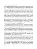
and then it is sealed with epoxy or metals [Wang and Esashi, 1997; Giachino et al., 1981, Peters in [Gia 81]].
Figure 3.12 illustrates the approach used by Wang and Esashi (1997). In another approach, sub-surface
polysilicon leads are used with the help of chemical–mechanical polishing to achieve a planar bonding sur-
face that allows a hermetic seal (Figure 3.13). This can be done at the wafer scale but results in substan-
tial parasitic capacitance, which may influence the choice of interface circuit [Chavan and Wise, 1997].
3.4.6 Design Variations
Anumber of variations to the conventional choices for structures and materials have been reported. These
include ultra-thin dielectric diaphragms, bossed or corrugated diaphragms, double-walled diaphragms
with embedded rigid electrodes, and structures with sense electrodes located external to the sealed cavity.
3-20 MEMS: Applications
Ground
Pyrex glass
Servo
electrode

Sensing
electrode
p
++
silicon
Metal layer
Diaphragm
FIGURE 3.12 Lead transfer in an electrostatically servo-controlled pressure sensor. (Reprinted with permission
from Wang, Y., and Esashi, M. [1997] “A Novel Electrostatic Servo Capacitive Vacuum Sensor,” Proc., IEEE
International Conference on Solid-State Sensors and Actuators [Transducers ’97], 2, pp. 1457–1460.)
© 2006 by Taylor & Francis Group, LLC
For achieving very high sensitivities, Equation 3.40 suggests that the area of the diaphragm should be
increased and the thickness should be decreased. However, a larger and thinner diaphragm develops high
stress under applied pressure, which may cause device failure. Dielectric materials compatible with silicon
processing have been explored as alternative structural materials for pressure sensors. In particular, stress-
compensated silicon nitride has been the focus of some interest. It is both chemically and mechanically
robust, with a yield strength twice that of silicon. High sensitivities were reached by using a large and thin sil-
icon nitride diaphragm of 2 mm diameter and 0.3 µm thickness [Zhang and Wise, 1994]. Silicon nitride is
under high tensile residual stress after LPCVD deposition, which reduces the diaphragm deflection. To
compensate this residual stress, a silicon dioxide layer, which contributes compressive stress, was used
between two silicon nitride layers (60 nm/180 nm/60 nm). To c o m p ensate the non-linear behavior due to
large deflections, a3µm thick boss (p
ϩϩ
Si) was located in the center of the diaphragm. Its diameter was
60% of the diaphragm; this percentage is generally a good compromise: agreater percentage lowers sen-
sitivity, a smaller percentage does not provide the fullest benefit toward linearity. The sensitivity was
10,000 ppm/Pa (5 fF/mTo r r), which is 10ϫ greater than the typical value for capacitive devices. The minimum
resolution pressure was 0.1 mTorr. The TCO and TCS were, respectively, 910 ppm/K and Ϫ2900 ppm/K.
The dynamic range was Ͼ130 Pa.
Introducing corrugation into a pressure sensor diaphragm allows a longer linear travel, and can con-

tribute toward larger dynamic range. Corrugations can be created by wet or dry etching. Ding (1992), and
Zhang and Wise (1994a) present bossed and corrugated diaphragms under tensile, neutral, and compres-
sive stress. Both papers report a square root dependence of deflection versus pressure for unbossed corru-
gated pressure sensors. Residual stress in the diaphragm can result in bending when corrugations are present
even in the absence of an applied pressure. The use of a boss in the center has been showntoconsiderably
improve this, but can cause a deflection in the opposite direction.
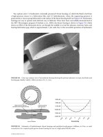
Wang et al. (2000) reported a differential capacitive pressure sensor consisting of a double-layer
diaphragm with an embedded electrode. As shown in Figure 3.14, one capacitor is formed between the
upper diaphragm and middle electrode, and another between the electrode and lower diaphragm, serving
as a capacitive half-bridge. The diaphragms are mechanically connected to each other, and move in the same
direction, which is dependent on the pressure difference between the upper and lower surfaces of the entire
structure. The advantage of this pressure sensor is that the sense cavity is sealed, but still can generate a sig-
nal based on differential pressure. In the reported effort, a diaphragm size of 150 ϫ 150µm
2
, thickness of
2 µm, and capacitor gaps of nominally 1µmwere used. With one side of the pressure sensor at atmosphere,
the nominal capacitance change is 86 fF for a differential pressure change from Ϫ80kPa to 80kPa.
Most masking steps in the fabrication of pressure sensors are consumed on electrical lead transfer from the
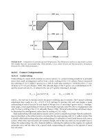
inside of the vacuum cavity to the outside as shown in the previous devices. A pressure sensor that elim-
inates the problem of the sealed lead transfer by locating the pick-off capacitance outside the sealed cavity
is illustrated in Figure 3.15 [Park and Gianchandani, 2000]. A skirt-shaped electrode extends outward
from the periphery of the vacuum-sealed cavity, and serves as the element which deflects under pressure.
The stationary electrode is metal patterned on the substrate below this skirt. As the external pressure
Micromachined Pressure Sensors: Devices, Interface Circuits, and Performance Limits 3-21
Tab contact
Glass substrate
SiO
2
/Si
3

N
4
/SiO
2
SiO
2
/Si
3
N
4
/SiO
2
Poly-Si
Poly-Si
Ti/Pt/Au
Ti/Pt/Au
P
++
Si
P
++
Si
External lead for
glass electrode
External lead to Si body
Dielectric
protection
Contact to upper Si body
Glass substrate
Silicon

(a) (b)
FIGURE 3.13 Sealed lead transfer for a capacitive pressure sensor using a sub-surface polysilicon layer. (Reprinted
with permission from Chavan, A.V., and Wise, K.D. [1997] “A Batch-Processed Vacuum-Sealed Capacitive Pressure
Sensor,” International Conference on Solid-State Sensors and Actuators [Transducers], pp. 1449–1451.)
© 2006 by Taylor & Francis Group, LLC
increases, the center of the diaphragm deflects downwards, and the periphery of the skirt rises, reducing
the pick-off capacitance. This deflection continues monotonically as the external pressure increases
beyond the value at which the center diaphragm touches the substrate, so this device can be operated in
touch mode for expanded dynamic range. To fabricate this, a silicon wafer was first dry etched to the
3-22 MEMS: Applications
Differential pressure
P
Sealed cavity
Silicone gel
d
1
− ∆d
C
1
+ ∆C
C
2
− ∆
C
d
2
+ ∆d
A B C
FIGURE 3.14 Differential capacitive pressure sensor with double-layer diaphragm and embedded rigid electrode.
(Reprinted with permission from Wang, C.C., Gogoi, B.P., Monk, D.J., and Mastrangelo, C.H. [2000] “Contamination

Insensitive Differential Capacitive Pressure Sensors,” Proc., IEEE International Conference on Microelectromechanical
Systems, pp. 551–555.)
G1
H
R1
R2
T2
T1
Substrate (glass)
Electrode
Sealed cavity
(volume V)
Deformable
skirt or flap
(silicon)
T3
G2

2

Vbias
X
Y
Z
FIGURE 3.15 Electrostatic attraction between the electrode and skirt opposes the deflection due to external pressure.
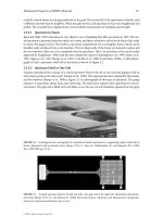
© 2006 by Taylor & Francis Group, LLC
desired height of the cavity, and then selectively diffused with boron to define the radius of the pressure
sensor. The depth of the boron diffusion determined the eventual thickness of the structural layer. The sil-
icon wafer was then flipped over and anodically bonded to a glass wafer that had been inlaid with a Ti/Pt
metal that serves as interconnect and provides the bond pads. The undoped Si was finally dissolved in

EDP, leaving the pressure sensor on the glass substrate. Fabricated devices are shown in Figure 3.16.
Numerical modeling indicates that for a device with diaphragm radius of 500 µm and total radius of
1 mm, cylinder height of 30 µm, uniform wall thickness of 5 µm, and nominal sense capacitor gap of
5 µm, the nominal capacitance is 3.86 pF and the sensitivity is about Ϫ2900 ppm/kPa in non-touch mode,
but drops to Ϫ270 ppm/kPa in touch mode.
Mastrangelo (1995) described a single crystal silicon pressure diaphragm using epitaxial deposition.
The advantage of this kind of sensor is that it does not require bonding on glass as most p
++
silicon pressure
sensors do, and the diaphragm stress condition and material properties are predictable, as single crystal
silicon provides more consistent performance than polysilicon.
3.4.7 Digital Compensation
One of the drawbacks of capacitive pressure sensors is their inherent non-linearity. Piezoresistive pressure
sensors offer better linearity without compensation, but these too need improvement for many applications.
Digital compensation involves the correction of the non-linearity in software of the digital interface (or
computer) by using polynomials or look-up tables. It is attractive because it is relatively easy to imple-
ment and reconfigure. Crary et al. (1990) described case studies involving the use of polynomials for com-
pensation of both capacitive and piezoresistive pressure sensors. In this effort, bi-variate compensation was
used to correct for changes in temperature and non-linearity of the response to pressure. First, the out-
put (response surface) of a pressure sensor was measured at a variety of fixed temperatures and pressures
as determined by other sensors, which were used as references. By averaging over a number of measure-
ments at each such point, it was determined that the deviation of the sensor response was 13 bits, which
could be regarded as the noise level. The compensation formula was then determined by using stepwise
regression to fit the response to a polynomial of the form P ϭ Σ
m,n
R
m
T
n
, where P is the actual pressure,

R is the sensor response, T is the temperature, and m and n are integers from 0–5. For a commercial
piezoresistive sensor, it was found that the standard error (taken as 1/4 of the 95% confidence interval)
was 4.6 bits using just the linear terms in the polynomial; but it improved to 9.7 bits with the inclusion
of higher-order terms which resulted in a polynomial of 7 terms. For a capacitive pressure sensor, a sim-
ilar effort resulted in standard errors of 4.6 and 7.5 bits, respectively.
3.4.8 Noise
Some of the noise sources in capacitive pressure sensors are similar to those presented previously in this chap-
ter for piezoresistive devices, but there are also some important differences. Equation 3.26 still holds for the
Micromachined Pressure Sensors: Devices, Interface Circuits, and Performance Limits 3-23
Skirt electrode
Diaphgram
Segmented skirt
electrode
Segmented skirt
electrode
Capacitor gap
FIGURE 3.16 SEM of fabricated devices from Park and Gianchandani (2003). (a) Device with continuous skirt elec-
trode. (b) Device with segmented skirt electrode. (c) Gap between skirt electrode and substrate. The metal thin film
on the substrate and the dummy anchor are also visible.
© 2006 by Taylor & Francis Group, LLC
noise from a circular diaphragm with built-in edges at low frequencies and low pressure, but within it
α
is now
1.2 instead of 1.7. The noise pressure due to viscous damping at higher pressures is obtained from Equation
3.27, as before. However, squeeze film damping in the small gap that generally exists between the deflect-
ing diaphragm and counter electrode can be a major contributor to diaphragm noise [Gabrielson, 1993]:
p
ෆ
2
ෆ

n
ෆ
ϭ 4kTR
sq
Ϸ 4kT(R
film
||R
perf
), where (3.47)
R
film
ϭ
΄ ΅
, and (3.48)
R
perf
ϭ
12
µ
A
2
΄
Ϫ Ϫ Ϫ
΅
N
π
d
3
(3.49)
In these equations, d is the average gap between the diaphragm and electrode, and

µ
is the viscosity of the
fluid between the plates (18 ϫ 10
Ϫ6
kg/m и s for air at 20°C). R
sq
is the damping coefficient due to squeeze
film damping. It can be approximated by the parallel combination (i.e., the product divided by the sum)
of damping coefficients R
film
and R
perf
. The former, Equation 3.48, is for damping between two
unperforated parallel plates; whereas the latter, Equation 3.49, is for damping between the diaphragm and
a perforated plate with N perforations and the fraction of open area in the plate represented by F. The for-
mer equation accounts for fluid flows only around the perimeter of the plate, whereas the latter one
accounts for flows only through the perforations.
As for piezoresistive pressure sensors, acoustic radiation can be described by Equation 3.49.
The electrical noise from the sensing piezoresistor is replaced by electrical noise from the sensing
capacitance. This is given by Chau and Wise (1987):
p
ෆ
2
ෆ
n
ෆ
ϭ
(3.50)
where C
0

is the sense capacitance and C
stray
is the parasitic capacitance in parallel with it. This mean square
pressure is proportional to h
6
g
3
/a
10
, i.e., it increases very rapidly as the sensor is scaled down in radius. It
should be noted that Equation 3.50 provides the broadband noise, which is diminished by the bandwidth
of the system in most cases.
In order to measure the readout capacitance in a pressure sensor, it is generally necessary to apply a
voltage bias between the electrode and the diaphragm. This bias may also be used to electrostatically pre-
deflect the diaphragm, and increase the nominal capacitance. However, electrical noise in the applied bias
will result in the application of instantaneous electrostatic forces, which can induce noise vibrations in
the diaphragm. Since this noise is dependent not only on the electrical source but also on the damped
temporal response of the diaphragm, it is not easily expressed by a closed-form equation.
The ability of the interface circuit to detect small changes in capacitance can impose an important
practical limitation of the usefulness of a pressure sensor. If ∆C
min
is the minimum resolvable capacitance
change for any given circuit, then the pressure resolution limit becomes:
Γ
ckt
ϭ
(3.51)
which is proportional to (h
3
g

2
/a
6
) [Chau and Wise, 1987].
3.4.9 Interface Circuits
There are several types of circuits that have been developed for interfacing with capacitive sensors. The two
most commonly used with pressure sensors are switched-capacitor charge amplifiers and capacitance-to-
frequency converters.
∆C
min
ᎏ
(C
0
S
cap
)
kT(C
0
ϩ C
stray
)
ᎏᎏ
(V
s
C
0
S
cap
)
2

3
ᎏ
8
lnF
ᎏ
4
F
2
ᎏ
8
F
ᎏ
2
N s
ᎏ
m
3
µ
A
2
ᎏ
2
π
d
2
3-24 MEMS: Applications
© 2006 by Taylor & Francis Group, LLC
Switched-capacitor charge amplifiers generally offer high sensitivity and immunity from parasitic
capacitance. They are based upon charge integrators. Acharge integrator can be made using operational
amplifiers, as illustrated in Figure 3.17a. For this, the output voltage is given nominally by:

V
out
ϭϪ
͵
t
tϭ0
v
i
(t)dt (3.52)
The sensor interface (Figure 3.17b) utilizes a two-phase clock to compare the variable sense capacitor (C
X
)
to a reference capacitor (C
R
) [Park and Wise, 1983]. Areset pulse initially nulls the output (Figure 3.17c).
Subsequently, when the clock switches, acharge proportional to the clock amplitude and the difference
between the reference and variable capacitor is forced into the feedback capacitor C
F
,producing an output
voltage given by:
V
out
ϭ
(3.53)
Since this scheme measures the difference between two capacitors, it is unaffected by parasitic capacitance
(C
P
) values that are common to both.
One concern related to the switched capacitor interface circuit is the switching noise caused by the
downward transition of the reset signal. Because the upward transition occurs after the output is sampled,

and causes the output to be nulled, it is not critical. The difficulty with the downward transition is that
since it is rapid, the charge stored in C
gs
, the capacitance between the gate and source of the reset transis-
tor, cannot immediately change in response to it, and this is reflected as a spike in the output signal. One
solution is to introduce a dummy transistor as shown in Figure 3.18. This transistor is sized to have a net
capacitance C
dummy
, that is the same as C
gs
.Its source and drain are shorted, so that it does not interfere
with the signal transmission. It is switched by a complement of the reset line, so that the downward spike
V
p
(C
X
Ϫ C
R
)
ᎏᎏ
C
F
1
ᎏ
RC
Micromachined Pressure Sensors: Devices, Interface Circuits, and Performance Limits 3-25
C
Gain
V
out

V
in
R
+
−
(a)
Reset
V
out
=
V
p
(CX − CR)/CF
Gain
+
−
−
(b)
CF
V−
Cps
CR
CX
V
p
V
p
0
0



V
out
(c)
Reset
CX1>CX2 CX2> CX3 CX3

t
FIGURE 3.17 (a) A simple integrator using an operational amplifier; (b) A switched capacitor charge integrator.
(Reprinted with permission from Park, Y.E., and Wise, K.D. [1983] “An MOS Switched Capacitor Readout Amplifier
for Capacitive Pressure Sensors,” Record of the IEEE Custom IC Conference); (c) A timing diagram for control and out-
put signals used in (b).
© 2006 by Taylor & Francis Group, LLC
on C
gs
appears as an upward spike across C
dummy
, and they effectively cancel each other out. If properly
designed, the dummy transistor can reduce the reset noise by an order of magnitude.
It is evident from the preceding discussion that despite the general simplicity and robustness of the
switched capacitor charge amplifier, it is (as any other interface circuit) susceptible to multiple sources of
electronic noise. Switched capacitor circuits, in general, suffer from switching noise that appears as spikes
in the voltage waveform at pulse edges (i.e., clock noise). One of the approaches used to combat this is
correlated double sampling (CDS), which is also commonly used as a signal processing method in CCD
image sensors [Hynecek, 1992]. This technique samples the input to the signal processing circuit block at
two different points in time, and produces a signal that is proportional to the difference between them. If
the input is switched between a reference null value and the actual signal value, noise components that
are common to both intervals will be automatically subtracted away. In this sense, the noise that can be
eliminated must be correlated between the two sample times. Generally, noise due to the power supply,
clock noise, and even kT/C noise can be cancelled in this manner. A simplified representation of the CDS

circuit is shown in Figure 3.19. It basically consists of a non-inverting amplifier of gain A, a unity gain
buffer, three sampling switches, and two storage capacitors. Initially, switches
φ
1 and
φ
2 are pulsed on,
while
φ
3 is not. This charges up capacitor C1 to a reference value V
s1
, while V
out
is held at ground. The
noise voltage is then stored in C1. In the second sample period,
φ
1 and
φ
3 are pulsed on, while
φ
2 is not.
If the input is stable at V
s
2
during this period, then V
out
settles at A(V
s
2
ϪV
s

1
), and the noise components
that are common to both sampling periods are cancelled out.
3-26 MEMS: Applications
V
p
0
V
p
0
CR
Cps
CX
CF
−


V−
Gain
−
+
V
out
=
V
p
(CX−CR)/CF
Reset
Reset
C

dummy
C
gs
FIGURE 3.18 Cancellation of reset switching noise by using a dummy transistor in a switched capacitor interface
circuit.
1
2
3
V
in
Va
C1
R1
R2
C2
Gain
+
−
Gain
+
−
Vc
V
out
Non-inverting gain stage
Vc = Va(1 + R2/R1)
FIGURE 3.19 Correlated double-sampling used to reduce noise, particularly in conjunction with the switched
capacitor charge amplifier interface circuit.
© 2006 by Taylor & Francis Group, LLC