The MEMS Handbook MEMS Applications (2nd Ed) - M. Gad el Hak Episode 1 Part 6 ppt
Bạn đang xem bản rút gọn của tài liệu. Xem và tải ngay bản đầy đủ của tài liệu tại đây (305.39 KB, 30 trang )
This chapter will adopt a classification of microactuators based on the form of the input energy and
will deal with only some of the microactuators listed in Table 5.4. In particular, piezoelectric, electro-
magnetic, shape memory alloys, and electrostatic microactuators will be discussed. Some information
will also be provided on polymeric, electrorheological, SMA polymeric, and chemical microactuators.
5.2 Piezoelectric Actuators
The discovery of the piezoelectric phenomena is due to Pierre and Jacque Curie, who experimentally
demonstrated the connection between crystallographic structure and macroscopic piezoelectric phe-
nomena and published their results in 1880. Their first results were only on the direct piezoelectric effect
(from mechanical energy to electric energy). The next year, Lippman theoretically demonstrated the exis-
tence of an inverse piezoelectric effect (from electric energy to mechanical energy). The Curie brothers then
gave value to Lippman’s theory with new experimental data, opening the way to piezoelectric actuators.
After some tenacious theoretical and experimental work in the scientific community, Voigt synthesized all
the knowledge in the field using a properly tensorial approach, and in 1910 published a comprehensive study
on piezoelectricity. The first application of a piezoelectric system was a sensor (direct effect), a submarine
ultrasonic detector, developed by Lengevin and French in 1917. Between the first and second World Wars
many applications of natural piezoelectric crystals appeared, the most important being ultrasonic trans-
ducers, microphones, accelerometers, bender element actuators, signal filters, and phonograph pick-ups.
During World War II, the research was stimulated in the United States, Japan, and Soviet Union, resulting
in the discovery of piezoelectric properties of piezoceramic materials exhibiting dielectric constants up to
100 times higher than common cut crystals. The research on new piezoelectric materials continued during
the second half of the twentieth century with the development of barium titanate and lead zirconate titanate
piezoceramics. Knowledge was also gained on the mechanisms of piezoelectricity and on the doping pos-
sibilities of piezoceramics to improve their properties. These new results allowed high performance and low
cost applications and the exploitation of a new design approach (piezocomposite structures, polymeric
materials, new geometries, etc.) to develop new classes of sensors and, especially new classes of actuators.
5-8 MEMS: Applications
TABLE 5.4 Classification of Microactuators Based on the Input Energy
Input Energy Physical Class Actuator
Electrical Electric and magnetic field Electrostatic
Electromagnetic
Molecular forces Piezoelectric
Piezoceramic
Piezopolymeric
Magnetostrictive
Electrostrictive
Magnetorheological
Electrorheological
Fluidic Pneumatic High pressure
Low pressure
Hydraulic Hydraulic
Thermal Thermal expansion Bimetallic
Thermal
Polymer gels
Shape memory effect Shape memory alloys
Shape memory polymers
Chemical Electrolytic Electrochemical
Explosive Pyrotechnical
Optical Photomechanical Photomechanical
Polymer gels
Acoustic Induced vibration Vibrating
© 2006 by Taylor & Francis Group, LLC
5.2.1 Properties of Piezoelectric Materials
A piezoelectric material is characterized by the ability to convert electrical power to mechanical power
(inverse piezoelectric effect) by a crystallographic deformation. When piezoelectric crystals are polarized
by an electric tension on two opposite surfaces, they change their structure causing an elongation or a
shortening, according to the electric field polarity. The electric charge is converted to a mechanical strain,
enabling a relative movement between two material points on the actuator. If an external force or
moment is applied to one of the two selected points, opposing a resistance to the movement, this “con-
ceptual actuator” is able to win the force or moment, resulting in a mechanical power generation (Figure
5.13). The most frequently used piezoelectric materials are piezoceramics such as PZT, a polycrystalline
ferroelectric material with a tetragonal-rhombahedral structure. These materials are generally composed
of large divalent metal ions; such as lead; tetravalent metal ions, such as titanium or zirconium (Figure
5.14); and oxygen ions. Under the Curie temperature, these materials exhibit a structure without a cen-
ter of symmetry. When the piezoceramics are exposed to temperatures higher than Curie point, they
transform their structure, becoming symmetric and loosing their piezoelectric ability.
Common piezoelectric materials are piezoceramics such as lead zirconate titanate (PZT) and piezoelec-
tric polymers such as polyvinylidene fluoride (PVDF). To improve the performance of piezoceramics, the
Microactuators 5-9
F
F
F
d
+
−
E
(a) (b) (c)
FIGURE 5.13 Inverse piezoelectric effect. An external force F is applied to a piezoelectric parallelepiped as in con-
figuration (a). When an electric tension generator gives power to the actuator, it results in a displacement d, as in con-
figuration (b). If the electric power is disconnected, the piezoelectric parallelepiped returns to its initial condition, as
in configuration (c).
FIGURE 5.14 Structure of a PZT cell under the Curie temperature. White particles are large divalent metal ions,
gray particles are oxygen ions, and the black particle is a tetravalent metal ion.
© 2006 by Taylor & Francis Group, LLC
research proposed new formulations, PZN–PT and PMN–PT. These new formulations extend the strain
from the 0.1%–0.2% (for PZT) to 1% (for the new formulations) and are able to generate a power den-
sity five times higher than that of PZT. Piezoelectric polymers are usually configured in film structures
and exhibit high voltage limits, but have low stiffness and electromechanical coupling coefficients.
Piezoceramics are much stiffer and have larger electromechanical coupling coefficients; therefore poly-
mers are not usually chosen as actuators.
We can use the constitutive equations to describe the relationship between the electric field and the
mechanical strain in the piezoelectric media:
S
ij
ϭ s
E
ijkl
T
kl
ϩ d
ijk
E
k
, i, j, k, l ∈ 1, 2, 3
(5.3)
D
i
ϭ d
ijk
T
jk
ϩ
ε
ij
T
E
j
where D is the three-dimensional vector of the electric displacement, E is the three-dimensional vector of the
electric field density, S is the second order tensor of mechanical strain, T is the second order tensor of
mechanical stress, s
E
is the fourth order tensor of the elastic compliance,
ε
T
is the second order tensor of the
permeability, and d is the third order tensor of the piezoelectric strain. Note, through a transposition, d
is related to d as that can be observed in the commonly used matrix form of the constitutive equation:
S
I
ϭ s
E
I,J
T
J
ϩ d
I,j
E
j
, i, j ∈ 1, 2, 3; I, J ∈ 1, 2 … 6 (5.4)
D
i
ϭ d
i,J
T
J
ϩ
ε
T
i,j
E
j
The first version of the constitutive equation is useful to explicate the dimensions of the tensors, while the
second is more concise. There are many ways of writing these equations: another interesting version
(Equation 5.5) gives the strain in terms of stress and electric displacement, introducing the voltage matrix
g and the
β
matrix:
S
I
ϭ s
I,J
D
T
J
ϩ g
I,j
E
j
, i, j ∈ 1, 2, 3; I, J ∈ 1, 2 … 6 (5.5)
E
i
ϭ Ϫg
i,j
T
J
ϩ
β
T
i,j
D
j
If the tensors/vectors D, S, E, and T are rearranged into nine-dimensional column vectors, the constitu-
tive equation can then take the form of Equation 5.6, Equation 5.7, Equation 5.8, or Equation 5.9, accord-
ing to the selection of dependent and independent variables:
Ά
D ϭ
ε
T
E ϩ d: T
S ϭ d
t
E ϩ s
E
: T
(5.6)
Ά
(5.7)
Ά
(5.8)
Ά
(5.9)
The above constitutive equations exhibit linear relationships between the applied field and the result-
ing strain. As an example, we can consider the tensor d. The experimental values of its components are
obtained by an approximation, as it depends upon the strain and the applied electric field. This approx-
imation consists of the hypothesis of low variation of applied voltage and the resulting strain. If the con-
sidered region is out of the field of linearity, then new values should be used to estimate the tensor d (the
constitutive equations are linear, but the value of d is different in each small considered region). Or, a
unique nonlinear constitutive equation could be used (d is no more constant but is a function of S and
E ϭ
β
S
D Ϫ h : S
T ϭ Ϫh
t
D ϩ c
D
: S
E ϭ
β
T
D Ϫ g : T
S ϭ g
t
D ϩ s
D
: T
D ϭ
ε
S
E ϩ e : S
T ϭ Ϫe
t
E ϩ c
E
: S
5-10 MEMS: Applications
© 2006 by Taylor & Francis Group, LLC
E, resulting in a theoretically correct but really complex approach). Another consideration is based on the
“aging effect” of piezoceramic materials represented by a logarithmic decay of their properties with time.
Therefore, over time, a new value of d should be estimated to obtain a correct model for the piezoceramic
material.
Considering linear constitutive equations (for each small region of the considered variables) in com-
bination with the hypothesis of low strain, we can write:
∇
s
v ϭ , with ∇
s
(o) ϵ
∇
o
ϩ ∇
o
T
(5.10)
where v is the speed of a basic element of piezoceramic. Using Equation 5.10, the equation of motion
(Equation 5.11), the Maxwell equations (Equation 5.12), and the previously mentioned constitutive
Equations 5.7 and 5.8 (the latter is used only to find the time derivative of D), we can obtain the general
Christoffel equations of motion (Equation 5.13).
∇oT ϭ
ρ
Ϫ F (5.11)
where
ρ
is the density of the material and F is the resulting internal force reduced to a surface force (with
the divergence theorem).
Ά
Ϫ∇ ϫ E ϭ
µ
0
∇H ϭ ϩ J (5.12)
where
µ
0
is the permeability constant, H is the electromagnetic induction, and J is current density.
Ά
∇oc
E
: ∇
S
v ϭ
ρ
Ϫ ϩ ∇oe
Ϫ∇ ϫ ∇ ϫ E ϭ
µ
0
ε
S
ϩ
µ
0
e:∇
S
ϩ
µ
0
(5.13)
In order to obtain a simple set of equations from Equation 5.13, we can neglect the presence of force, cur-
rent density, and the rotational term of E. The Fourier theorem allows us to transform, under reasonable
hypotheses, a periodical function (or in general a function defined into a finite time frame) into a sum of
trigonometric functions such that we can consider only a single wave propagating through the media.
The usual geometries of piezoelectric actuators are planar, therefore we will consider only planar waves
(Equation 5.14). Under these simplifications, we can obtain a simplified set of Christoffel equations
(Equation 5.15).
f(r,t) ϭ e
j(
ω
иtϪkIor)
(5.14)
where
ω
is the angular pulsation, I is the direction of the wave, and the constant k should be determined.
Ά
(5.15)
where V is the electric potential, while l
i
, l
j
, l
i,K
and l
Lj
are the matrices of the directional cosines. The
resulting equation can be solved to calculate the value of the potential energy to have a desired speed
(under the limitations of the used technology). Knowing the model for the actuating principle, this equa-
tion can be implemented in a more complex model of a complete actuator or it can be used as a
“metaphor” for the behavior of the actuator. The second approach allows the definition of a “virtual”
piezoelectric object implementing, through a proper calibration, some correction of the piezoelectric
matrix of the “real” piezoceramic to take into account some unconsidered phenomena.
Ϫk
2
(l
iK
c
E
KL
l
Lj
) и v
j
ϩ
ρω
2
v
i
ϭ Ϫj
ω
и k
2
(l
iK
e
Kj
l
j
) и V
ω
2
k
2
(l
i
ε
S
ij
l
j
) и V ϭ Ϫj
ω
и k
2
(l
i
e
iL
l
Lj
) и v
j
∂J
ᎏ
∂t
∂v
ᎏ
∂t
∂
2
E
ᎏ
∂t
2
∂E
ᎏ
∂t
∂F
ᎏ
∂t
∂
2
v
ᎏ
∂t
2
∂D
ᎏ
∂t
∂H
ᎏ
∂t
∂v
ᎏ
∂t
1
ᎏ
2
∂S
ᎏ
∂t
Microactuators 5-11
© 2006 by Taylor & Francis Group, LLC
5.2.2 Properties of Piezoelectric Actuators
In 2001, Niezrecki et al. in 2001 proposed a review of the state of the art of piezoelectric actuation. This
section will use this scheme and provide some explanations of the most common actuation systems.
Piezoelectric actuators are composed of elementary PZT parts that can be divided into three categories
(depending on the used piezoelectric relation) of axial actuators, transversal actuators, and flexural actu-
ators (Figure 5.15). Axial and transversal actuators are characterizedbygreater stiffness, reduced stroke,
and higher exertable forces, while flexural actuators can achieve larger strokes but exhibit lower stiffness.
Although we have shown in Figure 5.15 piezoelectric elementary parts with a parallelepiped shape,
piezoelectric materials are produced in a wide range of forms using different production techniques—from
simple forms, such as rectangular patches or thin disks, to custom very complex shapes. Because of the
reduced displacements, piezoelectric materials are not usually used directly to generate a motion, but are
connected to the user by a transmission element (Figure 5.2). Therefore, the piezoelectric actuators are
not just “simple actuators,” they are complete machines with an actuation system (the PZT element) and
a transmission allowing the transformation of mechanical generated power in a desired form. In fact, the
primary design parameters of a piezoelectric actuator (referring to the entire actuating machine, not only
the elementary PZT part) include
– the functional parameters — displacement, force, and frequency — and
– the design parameters — size, weight, and electrical input power.
Underlining only the functional parameters, the generated mechanical power is essentially a trade off
between these three parameters; the actuator architecture is devoted to increment one or two of these
5-12 MEMS: Applications
V
V
V
F
F
F
(a)
(b)
(c)
FIGURE 5.15 Elementary PZT part, where F is the exerted force and V is the electric potential difference between
two faces. (a) is an axial actuator, (b) is a transversal actuator, and (c) is a flexural actuator.
© 2006 by Taylor & Francis Group, LLC
parameters at the cost of the other parameters. Piezoelectric actuators are characterized by noticeable
exerted forces and high frequencies, but also significantly reduced strokes; therefore the architecture
designs aim to improve the stroke, reducing force or frequency. A distinction can then be made between
–force-leveraged actuators and
–frequency-leveraged actuators.
The leverage effect can be gained with an integrated architecture or with external mechanisms, so
another distinction can be made between
– internally leveraged actuators and
– externally leveraged actuators.
The most common internally force-leveraged actuators include:
(1) Stack actuators
(2) Bender actuators
(3) Unimorph actuators and
(4) Building-block actuators.
The externally force-leveraged actuators can be subdivided as:
(1) Lever arm actuators
(2) Hydraulic amplified actuators
(3) Flextensional actuators and
(4) Special kinematics actuators.
The frequency-leveraged actuators can be, in general, led back to inchworm architecture.
Stack actuators consist of multiple layers of piezoceramics (Figure 5.16). Each layer is subjected to the
same electrical potential difference (electrical parallel configuration), so the total stroke results is the sum
of the stroke of each elementary layer, while the total exertable force is the forceexertedby a single ele-
mentary layer. The leverage effect on the stroke is linearly proportional to the ratio between the elemen-
tary piezoelectric length and the actuator length.
The most common stack architectures can gain some microns stroke, exerting some kilonewtons
forces, with about ten microseconds time responses.
Bender actuators consist of two or more layers of PZT materials subjected to electric potential differ-
ences, which induce opposite strain on the layers (Figure 5.17). The opposite strains cause a flexion of the
bender, due to the induced internal moment in the structure. This architecture is able to generate an
amplification of the stroke as a quadratic function of the length of the actuator, resulting in a stroke of
Microactuators 5-13
V
F
s
S
FIGURE 5.16 Stack actuator. V is the electrical potential difference applied to each piezoelectric element, F is the
total exertable force. The stroke s of a single piezoelectric element is proportional to s, while the total stroke S is pro-
portional to S.
© 2006 by Taylor & Francis Group, LLC
more than one millimeter. Different configurations of bender actuators are available, such as end sup-
ported, cantilever, and many other configurations with different design tricks to improve stability or
homogeneity of the movement.
Unimorph actuators are a special class of bender actuators, which are composed of a PZT layer and a
non-active host. Two co mmon unimorph architectures are: Rainbow, developed by Heartling (1994) and
Thunder, developed at NASA Langley Research Center (Wise, 1998). These are characterized by a pre-
stressed configuration. Being stackable, they are able to gain important strokes (some millimeters).
Building block actuators consist of various configurations characterized by the abilitytocombine the
elementary blocks in series or parallel configurations to form an arrayed actuation system with improved
stroke by series arrays and improved force by parallel arrays. There are various state-of-the-art elemen-
tary blocks available such as C-blocks, recurve actuators, and telescopic actuators.
The first class of externally leveraged actuators to be examined is the lever arm actuator class. Lever
arm actuators are machines composed of an elementary actuator and a transmission able to amplify the
stroke and reduce the generated force. The transmission utilized is a leverage mechanism or a multistage
leverage system. To r e duce design complexity, the leverage system is generally composed of two simple
elements: a thin and flexible member (the fulcrum) and a thicker, more rigid, long element (the leverage
arm). Another externally leveraged architecture is hydraulic amplification. In this configuration, a piezo-
electric actuator moves a piston, which pumps a fluid into a tube moving another piston of areduced sec-
tion. The result is a very high stroke amplification (approximately 100 times); however, this amplification
involves some problems due to the presence of fluids, microfluidic phenomena, and high frequency
mechanical waves that are transmitted to the fluids. The third class of externally amplified actuators is
flextensional actuators. This class is characterized by the presence of a flexible component with a proper
shape, able to amplify displacement. It differs from the lever arm actuators approach, because of its
closed-loop configuration, resulting in a higher stiffness but reduced amplification power. To increment
the stroke amplification, this class of actuators can be used in a building-block architecture. Atypical
example is a stack of Moonie actuators. The research on actuation architecture is very dynamic. New
design solutions emerge in literature and on the market frequently; therefore it would be improper to
generalize these classifications based on only the three described classes of externally leveraged actuators:
lever arm, hydraulic, and flextensional.
The final class of externally leveraged actuators uses the frequency leverage effect. These actuators are
basically reducible to inchworm systems (Figure 5.18). In general, they are composed of three or more
actuators, alternatively contracting, to simulate an inchworm movement. The resulting system is a very
precise actuator, with very high stroke (more than 10mm), but with a reduced natural frequency.
The behavior of PZT actuators can be affected by undesired physical phenomena such as hysteresis. In
fact, hysteresis can account for as much as 30% of the full stroke of the actuator (Figure 5.19). An addi-
tional problem is the occurrence of spurious additional resonance frequencies under the natural fre-
quencies. These additional frequencies introduce undesired vibrations, reducing positioning precision
and the overall performance of the actuator. Furthermore, the depoling effect, which results in an unde-
sired depolarization of artificially polarized materials, occurs when a too-high temperature of the PZT is
gained, atoo-large potential is imposed to the actuation system, or a too-high mechanical stress is
applied. To avoid undesired phenomena, the actuator should be maintained within a proper range of
temperatures, mechanical stresses, and electrical potential. A design able to counteract such undesired
effects could be studied and a control system implemented. The piezoelectric effect could be implemented
5-14 MEMS: Applications
S
FIGURE 5.17 Bender actuator, where S is the total stroke.
© 2006 by Taylor & Francis Group, LLC
to sense mechanical deformations.With a very compact design, a controlled electromechanical system can
be developed. This is one of the many reasons piezoelectric actuators have become so successful.
5.3 Electromagnetic Actuators
5.3.1 Electromagnetic Phenomena
The research on electromagnetic phenomena and their ability to generate mechanical interactions is
ancient. The first scientific results were from William Gilbert (1600), who, in 1600, published De Magnete,
a treatise on the principal properties of a magnet — the presence of two poles and the attraction of oppo-
site poles. In 1750, John Michell (1751) and then in 1785, Charles Coulomb (1785–1789) developed a
quantitative model for these attraction forces discovered by Gilbert. In 1820, Oersted (1820) and inde-
pendently, Biot and Savart (1820), discovered the mechanical interaction between an electric current and
a magnet. In 1821, Faraday (1821) discovered the moment of the magnetic force. Ampere (1820) observed
a magnetic equivalence of an electric circuit. In 1876, Rowland (1876) demonstrated that the magnetic effects
due to moving electric charges are equivalent to the effects due to electric currents. In 1831, Michael
Faraday (1832) and, independently, Joseph Henry (1831) discovered the possibility of generating an elec-
tric current with a variable magnetic field. In 1865, James Clerk Maxwell (1865) developed the first com-
prehensive theory on electromagnetic field, introducing the modern concepts of electromagnetic waves.
Microactuators 5-15
(a) (b)
(c) (d)
(e)
(f)
(g)
FIGURE 5.18 Sequential inchworm movement.
Strain
Field
FIGURE 5.19 Hysteresis in PZT actuators.
© 2006 by Taylor & Francis Group, LLC
Though not considered so by his contemporaries, his theory was revolutionary, as it did not require the
presence of a media, the ether, to propagate the electromagnetic field. Later, in 1887, Hertz (1887) exper-
imentally demonstrated the existence of electromagnetic waves. This opened up the possibility of neglect-
ing the ether and, in 1905, aided the formulation of the theory of relativity by Albert Einstein (1905).
While electromagnetic physics was being studied, new advances in electromagnetic motion systems were
developed. The earliest experiments were undertaken by M.H. Jacobi (1835) in 1834 (moving a boat).
Though the first complete electric motor was built by Antonio Pacinotti (1865) in (1860). The first induc-
tion motor was invented and analysed by G. Ferraris (1888) in 1885 and later, independently, by N. Tesla
(1888), who registered a patent in the United States in 1888. Many other macro electromagnetic motors
were later developed and research in this field remained very active. Research in the field of electric
microactuators started in 1960 with W. McLellan, who developed a 1/64th inch cubed micromotor in
answer to a challenge by R. Feynman. Since then an indefinite number of inventions and prototypes have
been presented to the scientific community, patented, and marketed. Therefore, outlining the history of
microelectromagnetic actuators is an almost impossible task; however, by observing the new technologies
produced, we are able to trace the key inventions and ideas to the formation of actual components For
example, the isotropic and anisotropic etching techniques that were developed in the 1960s generated
bulk micromachining in 1982; sacrificial layer techniques also developed in the 1960s generated surface
micromachining in 1985. Some more recent technologies include silicon fusion bonding, LIGA technol-
ogy, micro electro, and discharge machining.
5.3.2 Properties of Electromagnetic Actuators
Electromagnetic actuators can be classified according to four attributes: geometry, movement, stroke, and
type of electromagnetic phenomena (Tables 5.5–5.8).
We will use the Lagrange equations of motion or Newtonian equations of motions to derive the mod-
els of each single type of actuator:
΄ ΅
Ϫ ϭ Q
i
, i ϭ 1,2… n (5.16)
Α
m
jϭl
F
j
(t, r) ϭ m
d
2
r
ᎏ
dt
2
∂(⌫ Ϫ ⌸)
ᎏᎏ
∂q
i
∂(⌫ ϩ D)
ᎏᎏ
∂q
.
i
d
ᎏ
dt
5-16 MEMS: Applications
TABLE 5.5 Classification of Electromagnetic Microactuators Based
on Geometry
Geometry of the Actuator
Planar
Cylindrical
Spherical
Toroidal
Conical
Complex shape
TABLE 5.6 Classification of Electromagnetic Microactuators Based
on Movement
Movement of the Actuator
Prismatic
Rotative
Complex movement
© 2006 by Taylor & Francis Group, LLC
where the first and second equation represents, respectively, Lagrangian and Newtonian approach; the
used symbols Γ, D, and Π denote, respectively, the kinetic, potential, and dissipated energies; while q
i
and
Q
i
represent, respectively, the generalized coordinates and the generalized forces applied to the system.
The Newtonian approach corresponds to the use of Newton’s second law of motion, where F
j
is a vecto-
rial force applied to the system, r is the vector representing the position and the geometrical configura-
tion of the system, and m is the mass of the system. The presence of rotary movement can imply the use
of an analogous rotary version of Newton’s second law. Multibody systems can be also considered with
the use of a simple and concise matrix method. To develop MEMS models, Γ, D, and Π, in the Lagrangian
approach, and F, in the Newtonian approach, should take account of mechanical and electrical terms.
We will first consider the Lagrangian approach as it is able to simply mix many forms of physical inter-
actions without separating the model into many parts. If we consider elementary mechanical movement
(prismatic and rotational) and elementary electric circuits, and then apply a lumped parameters model with
a Lagrangian approach, we can propose the synthetic Table 5.9, to associate each elementary parameter with
each kind of energy mentioned in (Equation 5.16) and select the correct generalized coordinates and forces.
The proposed table is mainly outlining many other forms of energy deemed worthy of consideration,
as well as other basic or complex models to be taken into account. For instance, the effect of impacts due
Microactuators 5-17
TABLE 5.7 Classification of Electromagnetic Microactuators Based
on the Stroke
Stroke of the Actuator
Limited stroke
Unlimited stroke
TABLE 5.8 Classification of Electromagnetic Microactuators Based on
Electromagnetic Phenomena
Electromagnetic Phenomena of the Actuator
Direct current microactuators
Induction microactuators
Syncronous microactuators
Stepper microactuators
TABLE 5.9 Selection of Terms for Lagrange Equations of Motion
Generalized Elementary Movement Terms of Lagrange Equation Elementary Lumped Parameter
Prismatic mechanical movement Kinetic energy m: mass (prismatic inertial term)
Potential energy k: linear stiffness
Dissipative energy f: linear friction
Generalized coordinate x: linear coordinate along the trajectory
Generalized force F: applied force
Rotational mechanical movement Kinetic energy J: moment of inertia
Potential energy k: rotational stiffness
Dissipative energy f: rotational friction
Generalized coordinate t: rotational coordinate along the trajectory
Generalized force T: applied torque
Electric circuit Kinetic energy L: selfinductance
M: mutual inductance
Potential energy C: capacitance
Thermal Dissipative energy R: resistance
Generalized coordinate q: electrical charge
Generalized force u: applied voltage
© 2006 by Taylor & Francis Group, LLC
to backlash between mechanical components can be considered introducing stiffness function, which are
governed by the distance between two consecutive components of the kinematical chain. The resulting
elastic force can be evaluated with the product of the stiffness function and the distance between the two
components. We consider this function as constant or polynomial function of the distance between the
two components; however, it assumes the value of zero when the absolute distance between the two con-
sidered consecutive components is less than a half of the backlash:
k
12
(x Ϫ y) ϵ k
12
ϩ
Ϫ
(5.17)
where k
12
is the modified stiffness function, x is the generalized position of a mechanical component of
the microactuator, y is the generalized position of the consecutive mechanical component, g is the back-
lash, and k
12
is the real stiffness of the junction between the two adjacent components (Figure 5.20).
In a similar way, the backlash can also be considered in the definition of the dissipative forces between
two adjacent components. The definition of the friction is a more complex problem, because of the pres-
ence of different type of frictions. Three important friction phenomena should be considered: Coulomb
friction, viscous friction, and static friction:
F ϵ
f
v
ϩ f
s
exp
Ϫ
ϕ
Έ
ξ
.
Έ
ϩ f
c
Έ
ξ
.
Έ
(5.18)
where f
v
, f
s
, f
c
and
ϕ
are optimal parameters, while
ξ
ϵ x Ϫ y is the relative position of two adjacent
mechanical components. The presence of backlash introduces a discontinuity in the frictional parameters
(Equation 5.19), and the situation can radically increment the complexity of the frictional model.
F ϵ
Ά
f
v
(l ϩ ∆
1
δ
(
ξ
)) ϩ f
s
(l ϩ ∆
2
δ
(
ξ
))exp
΄
Ϫ
ϕ
(1 ϩ ∆
3
δ
(
ξ
))Έ
ξ
.
Έ
΅
ϩ f
c
(1 ϩ ∆
4
δ
(
ξ
))Έξ
.
Έ
·
,
δ(
ξ
) ϵ
Ϫ
(5.19)
where ∆
1
, ∆
2
, ∆
3
, and ∆
4
are optimal parameters, which take into account the variation of frictional effects
in the “backlash-disconnected” joint. Many other observations can also be introduced to model a partic-
ular phenomenon such as the hysteretic behavior of general mechanical systems, but these remarks will
be considered only for shape memory microactuators. An example for electrical parameters is the
dependence of resistivity based on temperature (Equation 5.20). In fact, a fluctuation in the temperature
range due to unexpected phenomena and changes in internal temperature caused by electrical power
feeding and Joule effect affect the resistivity of a microelectromechanical system, and its related resist-
ance, thus altering its functionality.
ρ
ϭ
ρ
0
΄
1 ϩ
Α
n
iϭ1
α
i
(T Ϫ T
0
)
i
΅
(5.20)
|
ξ
ϩ g/2|
ᎏᎏ
ξ
ϩ g/2
|
ξ
Ϫ g/2|
ᎏᎏ
ξ
Ϫ g/2
1
ᎏ
2
|
ξ
.
|
ᎏ
ξ
.
|
ξ
.
|
ᎏ
ξ
.
|x Ϫ y ϩ g/2|
ᎏᎏ
x Ϫ y ϩ g/2
|x Ϫ y Ϫ g/2|
ᎏᎏ
x Ϫ y Ϫ g/2
k
12
ᎏ
2
5-18 MEMS: Applications
x−y
k
12
g/2
−g/2
k
12
FIGURE 5.20 Modified stiffness function to take account of backlash.
© 2006 by Taylor & Francis Group, LLC
where
ρ
is the resistivity,
ρ
0
is the reference resistivity, α
i
is the temperature dependence coefficient, T is
the temperature of the resistor, and T
0
is the reference temperature. Other examples of non-linearity in
the electrical parameters can be observed in non-linear components, such as diodes.
Regarding the general microelectromechanical model theory, a suitable approach allows the modeling
of electro-mechanical systems using a lumped parameter approach. If designers consider the general rela-
tions between magnetic, electric, and mechanical fields, and referring to the Maxwell’s equations, they
could eventually apply a finite element approach to improve the model’s power:
∇oE ϭ 0
∇oB ϭ 0
∇ ϫ E ϭ Ϫ (5.21)
∇ ϫ B ϭ
µε
5.3.3 DC Mini- and Microactuators
Because of thermal problems related with brush friction, DC microactuators are not the most viable choice
within the class of electromagnetic microactuators. To develop a complete model of the actuator, one can
select a cylindrical geometry, having a rotational movement and an unlimited stroke. One can also con-
sider a single conductive coil, which is turned on a cylindrical rotor, able to rotate around its axis. The coil
is also embedded in a magnetic field B and it is fed with an electric current as in Figure 5.21. Due to the
action of the magnetic field on the electric current, the coil is affected by the mechanical couple:
τ
ϭ i и A ϫ B (5.22)
where
τ
is the mechanically generated couple, A is the area vector perpendicular to the coil, and B is the
magnetic field intensity. We can now consider a set of ncoils equally spaced on the rotor, which are
affected by a set of p magnetic fields perpendicular to the rotor axis. The same current i is in all the coils,
and the electric potential of the rotor is applied to the coils by brushes, which are used to change the
direction of the current every half turn of the rotor. The rotor then, is subject to the force computed by:
τ
(
θ
) ϭ i и |A| и |B| и
Α
nϪ1
jϭ0
Α
pϪ1
kϭ0
Έ
cos
θ
ϩ
π
и
Έ
(5.23)
where
θ
is the angular coordinate which identifies the position of the rotor in respect to the microactua-
tor’s stator (Figure 5.22).
j и p ϩ k и n
ᎏᎏ
p и n
ѨE
ᎏ
Ѩt
ѨB
ᎏ
Ѩt
Microactuators 5-19
x
y
z
A
S
″
F
F
i
B
FIGURE 5.21 Coil with an area A, an electric current i and embedded in a magnetic field B.
© 2006 by Taylor & Francis Group, LLC
When the number of coils, and/or the number of magnetic fields, is sufficiently high, the mechanical
torque expression can be further simplified:
τ
ϭ i
и
|A||B|
и
n
и
(5.24)
Therefore, under the assumption that the magnetic field is generated by the stator’s current, the magnetic
torque can be expressed as the product of a constant term and two electric variables: the rotor’s and the
stator’s currents:
τ
ϭ k
s
и i и i
s
(5.25)
To obtain the value of the angular speed of the rotor, we assume the temporary disregard of dissipa-
tions and other “parasitic phenomena” due to their effect, only before and after the transformation from
electric to mechanical energy. For this reason, all the input electrical energy from the rotor is converted
into mechanical energy and the angular speed of the rotor can be expressed:
ω
m
ϭ e/(k
s
i
s
) (5.26)
where e is the rotor’s electrical potential. With the aid of the transformation equations (Equation
5.25–5.26), the microactuator behavior can be described from a standpoint of circuit’s approach as in
Figure 5.23.
2p
ᎏ
π
5-20 MEMS: Applications
i
s
i
B
s
FIGURE 5.22 Scheme of a DC microactuator, where B is the magnetic field intensity, i is the rotor’s current, and i
s
is the stator’s current used to generate the magnetic field.
R
r
i
r
L
r
ϩ
Ϫ
e
r
v
r
ϩ
Ϫ
R
s
i
s
L
s
v
s
ϩ
Ϫ
k
g
f
J
m
J
L
v
e
, c
e
r
c
r
v
L
, c
L
FIGURE 5.23 Circuit model of a DC microactuator. The subdivision takes place in three parts: (s) is the stator’s elec-
tric circuit, (r) is the rotor’s electric circuit, and (m) is the mechanical circuit of the rotor. (R) is the mechanical cir-
cuit of the rotor after the speed reduction stage integrated in the microactuator.
© 2006 by Taylor & Francis Group, LLC
The symbols mentioned in Figure 5.23 are summarized as follows:
(s) Stator’s circuit
v
s
is the stator’s electric potential
i
s
is the stator’s current
R
s
and L
s
are the resistance and the inductance of the stator
(r) Rotor’s circuit
v
r
is the rotor’s electric potential
i
r
is the rotor’s current
R
r
and L
r
are the resistance and the inductance of the rotor
e
r
is the rotor’s potential that linked with the rotor’s current, is transformed in mechanical power which
value is related with the stator’s current and with the theoretical motion speed:
e
r
ϭ k
s
i
s
α
.
e
(5.27)
where k
s
is the electric–mechanic transformation constant.
(m) Mechanical stage
τ
e
is the theoretic motor torque which depends upon the rotor’s and stator’s currents
τ
e
ϭ k
s
i
s
i
r
(5.28)
α
e
is the theoretic position of the rotor
J
m
is the motor’s inertia
J
L
is the load’s inertia
f is the reduced friction coefficient of the system as described in Equation 5.19
k is the reduced stiffness coefficient of the system as described in Equation 5.17
g is the reduced backlash coefficient of the system
α
R
is the theoretic position after the reduction stage (Equation 5.29)
α
L
is the position of the load
τ
L
is the applied torque of the load
α
e
ϭ
α
r
и r (5.29)
where r (Ͼ1) is the mechanical reduction ratio. With a simple circuit analysis, a lumped parameter model
of the microactuator can be obtained (Equation 5.30):
v
s
ϭ R
s
i
s
ϩ L
s
v
r
ϭ R
r
i
r
ϩ L
r
ϩ e
r
e
r
ϭ k
s
i
s
α
.
e
α
R
ϭ
α
c
/r
(5.30)
τ
e
ϭ k
s
i
s
i
r
τ
R
ϵ k(
α
R
Ϫ
α
L
) ϩ f(
α
.
R
Ϫ
α
.
L
)
τ
e
Ϫ
ϭ J
m
α
e
τ
R
Ϫ
τ
L
ϭ J
L
α
.
.
L
The result of the model in Equation 5.30 is a correct approximation of the non-linear model behavior of
the electromechanical microactuator after a proper definition of the considered parameters. If any of the
τ
R
ᎏ
r
di
r
ᎏ
dt
di
s
ᎏ
dt
Microactuators 5-21
Ά
© 2006 by Taylor & Francis Group, LLC
parameters of the model are not able to reach the desired predictive precision, more complex models
could be considered in order to take into account neglected phenomena. Considering the introduction of
fictitious mechanical compliances or electrical parasitic phenomena could be followed by a calibration
procedure ruled directly by real experimental results or by a finite element model. Should a model not be
implemented in a controlling algorithm, a finite element model can be directly used to provide good pre-
dictive result. Some useful finite element software are available on the market to achieve a proper model,
thus creating new finite element software is not necessary.
5.3.4 Induction Mini- and Microactuators
Induction actuators consist of a mobile and a static part and the transformation from electric to mechan-
ical energy due to the inductance of each part of the microactuator. This section will address a cylindrical
rotary actuator with unlimited stroke and, to simplify the analysis, only a common configuration is con-
sidered: a three phase, two pole actuation system. Figure 5.24 shows a rotary induction motor. The mobile
part (the rotor) has a cylindrical shape and is able to rotate around its axis; the static part (the stator) has
the same axis as the rotor and is separated from it by an air gap. Both are composed of ferromagnetic
material and incorporate lengthwise holes carrying conductive wires that are close to the air gap.
To develop a mathematical model of the dynamic behavior of the considered microactuator, it is nec-
essary to define a reference system and an angular variable, which identify the position of the rotor
(Figure 5.25). In particular where the variable
θ
I
defines the position of the i-th rotor’s winding (r
i
) in
respect to the first stator’s winding (s
1
):
θ
i
ϭ
θ
ϩ
i Ϫ 1
(5.31)
where
θ
is indicated in Figure 5.25, as the angle between s
1
and r
1
, and f is the number of phases. The
dynamic model can be generalized as a multi-pole micromachine for which the ideal actuator speed can
be calculated by:
θ
.
a
ϭ 2
θ
.
/p (5.32)
where p is the (even) number of poles,
θ
is indicated in Figure 5.25, and
θ
a
is the ideal position of the
actuator. Therefore, the dynamic electromagnetic behavior of the system can be described by the matrix
equation:
Ά
(5.33)
e ϭ R и i ϩ
ϕ
.
ϕ
ϭ L и i
2
π
ᎏ
f
5-22 MEMS: Applications
s
g
r
FIGURE 5.24 Physical scheme of rotary induction actuator. s, r, and g represent, respectively, the stator, the rotor,
and the gap.
© 2006 by Taylor & Francis Group, LLC
where the following vectors are described in Equation 5.34: the vector e of electric potential, the vector e
of electric currents, and the vector
ϕ
of magnetic fluxes; the matrix R of electric resistances is defined in
Equation 5.35; and the matrix L of inductances is defined in Equation 5.36.
e ϭ
[e
s1
e
s2
e
s3
e
r1
e
r2
e
r3
]
T
, i ϭ [i
s1
i
s2
i
s3
i
r1
i
r2
i
r3
]
T
,
ϕ
ϭ [
ϕ
s1
ϕ
s2
ϕ
s3
ϕ
r1
ϕ
r2
ϕ
r3
]
T
(5.34)
where the index associated to each element of the three vectors refer to the stator/rotor winding shown
in Figure 5.25.
R ϭ
΄ ΅
(5.35)
where R
s
and R
r
are, respectively, the stator and rotor winding resistances, while I(3) and 0(3) are, respec-
tively, the three-dimensional identity and zero matrixes.
L ϭ
΄ ΅
(5.36)
where the submatrixes L
1,1
and L
2,2
, respectively, of statoric and rotoric inductances are defined in
Equation 5.37, while the submatrixes L
1,2
and L
2,1
of mutual inductances are defined in Equation 5.38.
L
1,1
ϭ
΄ ΅
,
L
2,2
ϭ
΄ ΅
(5.37)
where L
s
and L
r
are the selfinductance of, respectively, each stator’s and each rotor’s winding, and M
s
and
M
r
are the mutual inductance of, respectively, two stator’s or two rotor’s windings.
L
1,2
ϭ L
T
2,1
ϭ [l
i, j
]
iϭ1…3, jϭ1…3
’
l
i,j
ϭ M
sr
cos
΄
θ
ϩ (j Ϫ i)
΅
(5.38)
where M
sr
is the mutual inductance between a stator’s and a rotor’s winding and
θ
is indicated in Figure
5.25. Coupled with the appropriate electric dynamics, and with consideration of speed reduction stage,
2
π
ᎏ
3
M
r
M
r
L
r
M
r
L
r
M
r
L
r
M
r
M
r
M
s
M
s
L
s
M
s
L
s
M
s
L
s
M
s
M
s
L
1,2
L
2,2
L
1,1
L
2,1
0(3)
I(3) и R
r
I(3) и R
s
0(3)
Microactuators 5-23
s
1
s
2
s
3
Ϫ1
s
1
s
Ϫ2
s
2
s
Ϫ3
s
3
s
r
1
r
2
r
3
Ϫ1
r
3
r
Ϫ2
r
1
r
Ϫ3
r
2
r
s
FIGURE 5.25 Definition of the position of the rotor’s windings: i
r
and j
s
represent, respectively, the ith rotor’s wind-
ing and the jth stator’s winding; r
i
and s
j
represent, respectively the axis of the ith rotor’s winding and the axis of the
jth stator’s winding, and
θ
is the angular position of the first rotor’s winding in reference to the position of the first
stator’s winding.
© 2006 by Taylor & Francis Group, LLC
the mechanical equilibrium equations (Equation 5.39) would develop in the complete micromechanical
model of the system.
Ά
(
τ
e
Ϫ ϭ J
m
θ
τ
R
Ϫ
τ
L
ϭ J
L
θ
L
(5.39)
τ
R
ϵ k(
θ
R
Ϫ
θ
L
) ϩ f(
θ
.
R
Ϫ
θ
.
L
)
where
τ
e
is the electric torque generated by the electromagnetic interaction (Equation 5.43),
τ
R
is torque
transferred by the compliance of the mechanical stage,
τ
L
is the torque of the load; J
m
and J
L
are, respec-
tively, the inertia of the motor and the inertia of the load; r (Ͼ1) is the mechanical reduction ratio; k and
f are, respectively the stiffness (Equation 5.17) and the friction (Equation 5.19) coefficient of the reduc-
tion stage;
θ
,
θ
R
and
θ
L
are, respectively, the theoretic position of the rotor, the theoretic position after the
reduction stage (Equation 5.40) and the position of the load.
θ
ϭ
θ
R
и
r (5.40)
The computation of the electric torque
τ
e
is then related to the calculation of the generated power:
p ϭ e
T
i
ϭ (R
i
ϩ
ϕ
.
)
T
i (5.41)
ϭ (i
T
R
T
i)
1
ϩ (i
T
L
.
T
i)
2
ϩ (i
T
L
.
T
i
)
3
where the e and i are, respectively the vector of the electric potentials and the vector of the electric cur-
rents (Equation 5.34), R is the matrix of the electric resistance (Equation 5.35),
ϕ
is the vector of mag-
netic fluxes (Equation 5.34), L is the matrix of inductances (Equation 5.36).The three resulting terms of
the power Equation 5.41 are, respectively, the electric power converted into heat, the electric power con-
verted into mechanical power, and the variation of electromagnetic power of the system. The second
term, the conversion of electric power into mechanical power, is used to obtain the electric torque
τ
e
;only
the evaluation of the time derivative of the transposed matrix of the inductances is required:
L
.
T
ϭ
΄ ΅
, L
12
ϭ [i
i,j
]
iϭ1…3, jϭ1…3
, i
i,j
ϭϪ
θ
.
и M
sr
sin
΄
θ
ϩ (j Ϫ i)
΅
(5.42)
Because the time derivative of the transposed matrix of the inductances is linearly dependent by the time
derivative of the angular position of the rotor, the electric torque is easily found by:
τ
e
ϭ (5.43)
5.3.5 Synchronous Mini- and Actuators
Synchronous microactuators consist of a mobile and a static part and the transformation from electric to
mechanical energy is due to inductance of each part of the microactuator. The denomination of “syn-
chronous machine” is due to the synchronization between the magnetic fields of the actual parts of which
the microactuator is comprised. To simplify the studies, a cylindrical rotary actuator with unlimited
stroke is taken into consideration and only a common configuration is analyzed: three-phase two-pole
actuation system. In Figure 5.26 a rotary synchronous actuators is shown: the mobile part (rotor) can
rotate around its axis, the static part (stator) has the same axis of the rotor, and it is separated from it by
a gap. The stator is composed of ferromagnetic material and is furnished with liner conductive wires,
while the composition of the rotor will be given in the following.
i
T
L
.
T
i
ᎏ
θ
.
2
π
ᎏ
3
L
.
21
0
0
L
.
12
τ
R
ᎏ
r
5-24 MEMS: Applications
© 2006 by Taylor & Francis Group, LLC
To develop a mathematical model of the dynamic behavior of the microactuator under consideration,
it is necessary to define a reference system and an angular variable that identifies the position of the rotor
(Figure 5.27). In particular, the position of the rotor in respect to the i-th stator’s winding (s
i
) is indicated
by the variable
θ
i
:
θ
i
ϭ
θ
ϩ (i Ϫ 1) (5.44)
where
θ
indicated in Figure 5.27, is the angle between s
1
and d,while f is the number of phases.
In mathematical terms, the dynamic electromagnetic behavior of the system can be described by the
matrix equation 5.45, which takes the same form as the Equation 5.34.
Ά
e ϭ
[
e
s1
e
s2
e
s3
e
e
0 0
]
T
, i ϭ
[
i
s1
i
s2
i
s3
i
e
i
D
i
Q
]
T
,
ϕ
ϭ
[
ϕ
s1
ϕ
s2
ϕ
s3
ϕ
e
ϕ
D
ϕ
Q
]
T
(5.45)
where the vector e, i and
ϕ
represent, respectively, the electric potential, the electric current and the mag-
netic flux, the matrix R of the electric resistance and the matrix L of the inductance are defined in
Equation 5.46. The indices s1, s2, and s3 associated with each element, refer to the stator’s winding shown
in Figure 5.27. The index e is associated with the excitation winding on the rotor (Figure 5.28), while the
indices D and Q are, respectively, associated with the equivalent damping circuits of the direct and quad-
rature axis (Figure 5.29).
e ϭ R и i ϩ
ϕ
.
ϕ
ϭ L и i
2
π
ᎏ
f
Microactuators 5-25
s
g
r
s
n
FIGURE 5.26 Physical scheme of rotary synchronous actuator: s, r, and g represent, respectively, the stator, the rotor,
and the gap between them.
s
1
s
2
s
3
Ϫ1
s
1
s
Ϫ2
s
2
s
Ϫ3
s
3
s
s
s
n
q
d
FIGURE 5.27 Definition of the rotor’s position: i
s
represents the ith stator’s winding; s
i
represents the axis of the ith
stator’s winding; d and q are, respectively, the direct and the quadrature magnetic axis, while
θ
represents the angular
position of the direct magnetic axis in reference to the position of the first stator’s winding.
© 2006 by Taylor & Francis Group, LLC
5-26 MEMS: Applications
R ϭ Diag(R
s
, R
s
, R
s
, R
e
, R
D
, R
Q
), L ϭ
΄ ΅
(5.46)
where Diag(xx) is the diagonal matrix, while R
s
, R
e
, R
D,
and R
Q
are, respectively, the resistance of the sta-
tor’s winding, the excitation’s winding, the direct axis winding, and the quadrature axis winding. The sub-
matrixes L
1,1
, L
2,2
, L
1,2
and L
2,1
are defined in Equations 5.47–5.49.
L
1,1
ϭ [l
i,j
]
iϭ1…3, jϭ1…3
’
l
i,j
ϭ
Ά
l
0
ϩ L
00
ϩ L
2
cos
΄
2
θ
Ϫ (i Ϫ 1)
΅
, i ϭ j
Ϫ ϩ L
2
cos
΄
2
θ
Ϫ (5 Ϫ i Ϫ j)
΅
, i j
(5.47)
where l
0
is the statoric dispersion selfinductance, L
00
is the net statoric selfinductance, and L
2
is the ampli-
tude of the second Fourier term of each self-inductance of the stator.
L
2,2
ϭ
΄
΅
(5.48)
where L
e
, L
D
and L
Q
are, respectively, the excitation, the direct axis and the quadrature axis selfinductance,
while L
eD
is the mutual inductance between excitation and direct axis windings.
L
1,2
ϭ L
T
2,1
ϭ
[
l
i,j
]
iϭ1…3, jϭ1…3
’
l
i,j
ϭ
Ά
L
mf
cos(
θ
i
), j ϭ 1
L
mD
cos(
θ
i
), j ϭ 2 (5.49)
ϪL
mQ
sin(
θ
i
) j ϭ 3
0
0
L
Q
L
eD
L
D
0
L
e
L
eD
0
4
π
ᎏ
3
L
00
ᎏ
2
4
π
ᎏ
3
L
1,2
L
2,2
L
1,1
L
2,1
s
n
q
d
FIGURE 5.28 Excitation winding on the rotor.
1
r
q
d
Ϫ1
r
Ϫ2
r
2
r
FIGURE 5.29 Equivalent damping windings on the rotor. The electromagnetic characteristics of the two rotor’s
windings are projected on the quadrature and direct axes to form two equivalent virtual windings.
© 2006 by Taylor & Francis Group, LLC
where L
mf
, L
mD
and L
mq
are the maximum values of the mutual inductance between the rotor’s and sta-
tor’s windings. The electric couple exerted by the actuator can be calculated, as in Equations 5.41 and
5.43, considering electric input power converted into mechanical power divided by the angular speed.
The resulting real mechanical torque can be obtained with an equilibrium equation, like Equation 5.39,
which takes into consideration the friction, stiffness, and backlash of the mechanical components.
5.4 Shape Memory Actuators
The first known study on shape memory effect is credited to Olander (1932) who observed that an object
made of a Au–Cd alloy, if plastically deformed and then heated, is able to compensate the plastic defor-
mation and to recover its original shape. In 1938, Greninger and Mooradian (1938), changing the tem-
perature of a Cu–Zn alloy, observed the formation of a crystalline phase. In 1950, Chang and Read (1951)
used an X-ray analysis to understand the phenomenon of crystalline phase formation in shape memory
alloys and, in 1958, they showed the first shape memory Au–Cd actuator. An important milestone in the
development of the shape memory alloys was reached by researchers at the Naval Ordanance Laboratory
in 1961 lead by Buehler (1965), who observed the same shape memory effect in a Ni–Ti alloy. Ni–Ti alloys
are cheaper, easier to work with, and less dangerous than Au–Cd alloys. Many applications appeared on
the market during the 1970s: these were initially static in nature, but were later followed by dynamic
examples, thus starting the era of smart technology in microactuators.
Control techniques were later developed to improve performance, with a particular focus on reducing
cooling and heating time. Further data were acquired in reference to the properties of different shape
memory alloys. These new results, along with the ability to mass-produce Ni–Ti microelements, will be a
key to open the door to a much wider usage of smart materials. During the last two decades of the twen-
tieth century, many advances have been made in the modeling of SMA behavior, including the control in
regard to the change of shape; new design approaches to improve performances, particularly response-
time and reliability; and allowing for low cost mass production. For instance, the response time of the sys-
tem was significantly reduced by observing the relationship between the geometry of the system, its
thermal inertia, and the use of particular material combinations to generate a Peltier cell.
The reliability of a SMA is based on the knowledge of the physical properties of the alloy: this knowledge
is useful to prevent irreversible damages and to guarantee a repeatable behavior. The aims of preventing
damage and gaining repeatable behavior, were attained through experimental works with new simple and
complex models, varying design techniques, and the development of precise inputs and control of heating
feeding. Advances in the control segment are some of the most important aspects of SMA systems in order
to enhance repeatable high-speed and high-precision performance of such micro-SMA machines. Such
advances were made possible through new forms of power, spurred by research in production technology.
The consequential cost reduction of SMA objects followed shortly, thus allowing for the mass production
of industrial and medical applications. Arguably a suitable choice in the marketplace, SMA systems provide
new study opportunities placing alternate instruments in the designer’s hands for new applications.
5.4.1 Properties of Shape Memory Alloys
A shape memory alloy that deforms at a low temperature will regain its original undeformed shape when
heated to a higher temperature. This behavior is due to the thermoelastic martensitic phase transforma-
tion and its reversal (Bo and Lagoudas 1999a); the martensitic phase consists in a thick arrangement of
crystallographic planes, characterized by a high relative mobility. Many alloys exhibit shape memory
effect and the level of commercial interest of each and every alloy is correlated with its ability to easily
recover its initial position or to exert a significantly high force. Based on these criteria the SMA transfor-
mation of a Ni–Ti alloy is an interesting consideration. When a Ni–Ti alloy is subject to an external force,
the various planes will slide without a break in the crystallographic connections; the atoms of the struc-
ture are subject only to a reduced movement and through a subsequent heating, it will revert the struc-
ture to its initial position, resulting in the production of a significantly high mechanical force.
Microactuators 5-27
© 2006 by Taylor & Francis Group, LLC
The martensitic phase can appear in two different forms, depending on the history of the material.
Tw inned martensite is derived from the austenitic phase with cooling and it has a herringbone pattern,
while detwinned martensite is due to a sliding of the crystallographic planes. A scheme of a simple cycle
of transformations able to exhibit the shape memory effect is shown in Figure 5.30: aNi–Ti bar with a
fixed end and a free end without any external load is considered, apart from the thermomechanical loads
imposed during the transformations (A), (B), and (C) to generate the shape memory effect. The first con-
dition of the material (a) is the austenitic phase, after an external cooling (A), the material is converted
into twinned martensite (b). From a macroscopic viewpoint, we cannot observe any deformation of the
material or any external force exerted by the bar. Then a mechanical traction is applied to the bar (B) and
some portions of the bar are converted, during its elongation, into detwinned martensite (c). Finally, after
an external heating (C), the material is converted again into austenite and the bar recovers its original
shape.
It should be observed that the martensitic generation process does not require an introduction of
external substances and it depends only on the achievement of a critical temperature (M
s
,or martensite
start). The second important aspect of this transformation is the heat production, and finally an hys-
teretic phenomenon is observed when, at the same temperature, an austenitic phase and a martensitic
phase coexist. The austenite-to-martensite transformation is subdivided in two subsequent stages: Bain
strain and lattice-invariant shear (Figure 5.31). Bain strain generates, from austenite (a) and through a
movement of the plane interface, a martensitic structure (m
b
), then the lattice-invariant transformation
can generate a reversible deformation with a twinning (m
s1
) or a permanent deformation with a slip
(m
s2
). Areversible deformation is needed to exhibit a shape memory effect, so it is important to avoid
slipped martensite (m
s2
) and to generate twinned martensite (m
s1
).
From a macroscopic viewpoint, the martensitic formation can be represented in the temperature dia-
gram (Figure 5.32). Even though austenitic and martensitic macroscopic properties are slightly different,
the martensitic fraction can be used as the dependent variable to define the behavior of the shape mem-
ory material. An interesting characteristic of this diagram is the hysteresis, which can occur between
20–40°C and is associated with the micro-frictions within the structure.
The classical shape memory effect consists in the cycle of Figure 5.30 and is usually called one-way
shape memory effect (OWSM), because the shape transformation can be thermally commanded during
the martensite-to-austenite conversion. This is because the material is able to “remember” only the
austenitic shape. A more complete shape memory effect is the two-way memory effect (TWSM), which
consists of the ability of recovering an austenitic shape as well as a martensitic shape. This second phenom-
enon results in reduced forces and deformations, so it is not very common in commercial applications.
5-28 MEMS: Applications
(a)
(b)
(c)
(A)
(B)
(C)
FIGURE 5.30 Shape memory effect.
© 2006 by Taylor & Francis Group, LLC
TWSM can be obtained from a shape memory alloy after a thermomechanical training, which generates
a new microstructure (stress-biased martensite) and reduces the mechanical properties of the material.
The microscopic and macroscopic properties of the Ni–Ti alloys can be changed opportunely by varying
the percentage of Ni or introducing additive components (Table 5.10). An increment in the percentage of
Ni can reduce critical temperatures and increment the austenitic breaking stress. Fe and Cr are used to
reduce critical temperatures. Cu reduces the hysteretic cycle and decreases the stress that is necessary to
deform the martensite. O and C are usually avoided because they diminish the mechanical performance.
Microactuators 5-29
(a)
(m
b
)
(m
s1
) (m
s2
)
FIGURE 5.31 Martensite formation.
M
f
A
s
M
s
A
f
0
1
H
C
T
f
m
FIGURE 5.32 Martensitic fraction versus temperature. M
s
, M
f
, A
s
and A
f
are, respectively, martensite start, martens-
ite finish, austenite start, and austenite finish critical temperatures. H and C are, respectively, heating and cooling
transformations.
© 2006 by Taylor & Francis Group, LLC
Some thermomechanical treatments are necessary to induce a proper shape memory effect, however,
since shape memory alloys are commercialized after intermediate treatments, a classification such as in
Table 5.11 can be used to select the correct SMA component.
To induce the shape memory effect, an austenitic shape must be “saved.” This can be obtained through
a thermal treatment consisting of a heating of the cold processed component in a hot mould to over
400°C for several minutes. Hardening will then result after a rapid cooling. The TWSM can also be
obtained through a more complex approach consisting of the cyclic repetition of cold and hot deforma-
tions, which allows the “saving” of an austenitic shape as well as of a martensitic shape. Unfortunately, the
TWSM process will lead to a degradation of mechanical performance. If compared with the OWSM, the
recoverable deformation is only 2% (versus 5%–8%). In addition, its maximum stress is significantly
reduced, SME disappears if the temperature of the material exceeds 250°C, and it is time-unstable; con-
sequently the TWSM mechanical performance cannot be guaranteed after a high number of load cycles.
It should be noted that not only Ni–Ti exhibit SMA; some Cu alloys can be used, such as CuZnAl or
CuAlNi and others with Mn, as well as some Fe alloys (FePt, FePd, and FeNiCoTi). However, the descrip-
tion of their characteristics is beyond the scope of this chapter.
5.4.2 Thermoelectromechanical Models of SMA Fibers
The characteristics of SMA components can be estimated using different methods. Some of them include:
differential scanning calorimetry (DSC), liquid bath, resistivity measure, cycle with constant applied load,
and traction test. The DSC technique is able to measure absorbed and released heat in a SMA specimen
during crystallographic transformations. Liquid bath is a liquid with a controllable temperature in which
a SMA specimen is immersed and the imposed temperature is related to the macroscopic shape conver-
sion. Resistivity measure is based on the change of resistivity during crystallographic transformation. An
austenite–martensite–austenite cycle can be imposed with a constant mechanical load, allowing the mea-
sure of maximum and minimum deformations, which can be associated with critical points of the trans-
formations. A traction test can be executed at a constant temperature to measure mechanical properties
of the material and to relate them to the fixed temperature. The numerical characterization of the alloy
can be used to properly set a thermoelectromechanical dynamic model, which allows the open-loop con-
trol of the SMA used as an actuator. This chapter will consider only dynamic-kinematic models of fibers.
Designing dynamic models of SMA fibers is an active field and a classification of the different
approaches could be helpful in choosing the correct modelizing method. One classification can be based
5-30 MEMS: Applications
TABLE 5.10 Standard NiTi Alloys
Alloy code A
s
(°C) A
f
(°C) Composition (%)
S Ϫ5 ÷ 15 10 ÷ 20 ϳ55.8 Ni
N Ϫ20 ÷ Ϫ5 0 ÷ 20 ϳ56.0 Ni
C Ϫ20 ÷ Ϫ5 0 ÷ 10 ϳ55.8 Ni, 0.25 Cr
B 15 ÷ 45 20 ÷ 40 ϳ55.6 Ni
M 45 ÷ 95 45 ÷ 95 55.1 ÷ 55.5 Ni
H Ͼ95 95 ÷ 115 Ͻ55.0 Ni
TABLE 5.11 Some Common Commercial SMA Components
Treatment Description Characteristics
Cold processed The client execute thermal treatment Do not exhibit SME
Straight annealed Thermal treatment is executed by producer Wire exhibiting SME
Flat annealed Thermal treatment is executed by producer Plate exhibiting SME
Special annealed Thermal treatment is executed by producer Special shape exhibiting SME
© 2006 by Taylor & Francis Group, LLC
on deriving principles such as empirical models, micromechanical models, and thermodynamical mod-
els. Some models are directly structured to describe the behavior of SMA fibers (a one-dimensional prob-
lem), while other models are developed for more complex problems (two- or three-dimensional
problems) and then are reduced to describe only the characteristics of a one-dimensional problem.
Dynamic SMA models are usually composed by a stress-strain relationship and a kinematic law. We can
distinguish models where these two laws are inseparable, separable but coupled, or separable and uncou-
pled. The majority of the models are numerical because of the high non-linearity of the shape memory
effect; however simplified analytic models do exist. Despite their imprecision, analytic models are very
useful for a first dimensioning of a microactuator and in closed-loop applications. Many other distinc-
tions can be considered such as the presence of martensite variants in 3-D models or the set of inde-
pendent variables of the model. However, the proposed taxonomy can be a good starting point to deepen
the world of shape memory models. This chapter will describe a famous numeric model that was started
with a work of Tanaka (1986), first modified by Liang and Rogers (1990), and later by Brinson (1993),
while Brailoyski et al. (1996) and Potapov and da Silva (2000) added some interesting simplified analytic
models.
A simple micromechanical derivation of the first model was proposed by Brinson and Huang (1996).
A parallel Voigt model of austenite and martensite phases is considered in a one-dimensional specimen,
as in Figure 5.33. The specimen is subject to an external stress, so an elastic strain appears and, due to the
Microactuators 5-31
C
O″
FIGURE 5.33 SMA Voigt model where (M) is the martensite phase, and (A) is the austenite phase.
© 2006 by Taylor & Francis Group, LLC
considered Voigt model, the relations between austenite and martensite stress and strain are:
σ
ϭ (1 Ϫ
ξ
)
σ
a
ϩ
ξσ
m
ε
m
ϭ
ε
a
σ
a
ϭ E
a
ε
a
σ
m
ϭ E
m
ε
m
(5.50)
where
σ
is the stress of the specimen,
ξ
is the martensite fraction,
σ
a
and
σ
m
are, respectively, austenite and
martensite stress,
ε
a
and
ε
m
are, respectively, austenite and martensite strain, while E
a
and E
m
are, respec-
tively, austenite and martensite Young modulus. Relations in Equation 5.50 can be combined to obtain:
σ
ϭ [
ξ
и E
m
ϩ (1 Ϫ
ξ
) и E
a
] и
ε
a
(5.51)
Now consider a temperature increment able to generate a phase transformation: it results in an adjust-
ment of the SMA Voigt model (Figure 5.34) and the consequential total strain is the sum of the elastic
strain and of the transformation strain, thus the stress-strain relation can be modified as:
σ
ϭ [
ξ
и E
m
ϩ (1 Ϫ
ξ
) и E
a
] и (
ε
Ϫ
ε
L
и
ξ
S
) (5.52)
where
ε
L
is the maximum residual strain of the transformation and
ξ
S
is the detwinned martensite fraction.
The stress–strain relation (Equation 5.52) must be coupled with a kinetics equation:
Ά
ξ
ϭ cos
Ά ΄
σ
Ϫ
σ
cr
f
Ϫ C
M
(T Ϫ M
S
)
΅·
with T Ͼ M
S
,
σ
cr
S
ϩ C
M
(T Ϫ M
S
) Ͻ
σ
Ͻ
σ
f
cr
ϩ C
M
(T Ϫ M
S
) (5.53)
π
ᎏ
σ
S
cr
Ϫ
σ
f
cr
1 Ϫ
ξ
0
ᎏ
2
5-32 MEMS: Applications
C
0″
0
t″
FIGURE 5.34 SMA Voigt model where (M) is the martensite phase, (A) is the austenite phase, and (M
t
) is the trans-
formed martensite.
© 2006 by Taylor & Francis Group, LLC