The MEMS Handbook MEMS Applications (2nd Ed) - M. Gad el Hak Episode 2 Part 1 ppt

This chapter will address how to approach identifying microscale and mesoscale vacuum pumping
capabilities, consistent with the volume and energy requirements of meso- and microscale instruments
and processes. The mesoscale pumps now available are discussed. Existing microscale pumping devices
are not reviewed because none are available with attractive performance characteristics (a review of
the attempts has recently been presented by Vargo, 2000; Young et al., 2001; Young, 2004; see also
NASA/JPL, 1999).
In the macroscale world, vacuum pumps are not very efficient machines, ranging in thermal efficien-
cies from very small fractions of one percent to a few percent. They generally do not scale advantageously
to small sizes, as is discussed in the section on Pump Scaling. Because there is a continuing effort to
miniaturize instruments and chemical processes, there is not much desire to use oversized, power inten-
sive vacuum pumps to permit them to operate. This is true even for situations where the pump size and
power are not critical issues. Because at present microscale pump generated vacuums are unavailable,
serious limits are currently imposed on the potential microscale applications of many high performance
analytical instruments and chemical processes where portability or autonomous operations are necessary.
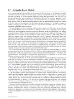
To illustrate this point, the performance characteristics of several types of macroscale and mesoscale
vacuum pumps are presented in Figure 8.1 and Table 8.1. Pumping performance is measured by Q
.
/N
.
,
which is derived from the power required, (Q
.
,W), and the pump’s upflow in molecules per unit time
(N
.
, #/s). Representative vacuum pumping tasks are indicated by the inlet pressure, p
I
, and the pressure ratio,
℘, through which N
.
is being pumped. The reversible, constant temperature compression power required

per molecule of upflow (Q
.
/N
.
) as a function of ℘ is depicted in Figure 8.1. The adiabatic reversible (isen-
tropic) compression power that would be required is also shown in Figure 8.1. The constant temperature
comparison is most appropriate for vacuum systems. Note the 3- to -5 decade gap in the ideal Q
.
/N
.
and
the actual values for the macroscale vacuum pumps. For low pump inlet pressures the gases are very
dilute and high volumetric flows are required to pump a given N
.
. The result is relatively large machines
with significant size and frictional overheads. Unfortunately, scaling the pumps to smaller sizes generally
increases the overhead relative to the upflow N
.
.
The current state of the art in mesoscale vacuum pump technology has been achieved primarily by
shrinking macroscale pump technologies. A closer look at the two technologies that have recently been
successfully shrunk to the mesoscale — diaphragm pumps and scroll pumps — will demonstrate the scal-
ing possibilities of macroscale pump technologies. A KNF Neuberger diaphragm pump (DIA) is an
example of a mesoscale diaphragm gas roughing pump. The diaphragm pump occupies a volume of
973 cm
3
, consumes 35 Watts of power, has a maximum pumping speed of 4.8 L/s, and reaches an ultimate
8-2 MEMS: Applications
SP
PER

RB
CL
RV
DR
1.E+00
1.E+02
1.E+04
1.E+06
1.E+08
1.E+10 1.E+12
1.E−22
1.E−21
1.E−20
1.E−19
1.E−16
1.E−17
1.E−18
1.E−15
1.E−14
1.E−13
1.E−12
Q
N
DDP(1 stage)
DDP(30 stages)
DIA
TM-4
DIF
SCL-2
TM-2

T/DR
ORB
SCL
SCW
Isentropic
Reversible & isothermal
Group 3
Group 2
Group 1
℘
FIGURE 8.1 Representative performance (Q
.
/N
.
) of selected macro- and mesoscale vacuum pumps (from Table 8.1)
as a function of pressure ratio (℘).
© 2006 by Taylor & Francis Group, LLC
pressure of 1.5 Torr. The energy efficiency of the diaphragm pump, 1.6 ϫ 10
Ϫ18
W/#/s, is consistent with
the energy efficiency of macroscale pumps operating with the limited pressure ratio, ℘ ϭ 100. Similar
diaphragm pumps are available at smaller sizes, but with ever increasing ultimate pressures.
Honeywell is currently developing the smallest published mesoscale diaphragm pump, the Dual
Diaphragm Pump (DDP) [Cabuz et al., 2001]. A single stage of the DDP measures 1.5 cm ϫ
1.5 cm ϫ 0.1 cm, and is manufactured using an injection molding process. The pump is driven by the
controlled electrostatic actuation of two thin diaphragms with non-overlapping apertures in a sequence
that first fills a pumping chamber with gas, and then expels the gas from the chamber. The DDP has a
pumping speed of 30 sccm at a power consumption of 8 mW. It is, however, only able to maintain a max-
imum pressure difference of 14.7 Torr per stage, making it strictly a low pressure ratio pump. Cascades of
thirty stages have been manufactured to increase the total pressure ratio; the corresponding energy effi-

ciency is given in Figure 8.1. This again illustrates the capability of making mesoscale diaphragm pumps,
but with ever increasing ultimate pressures as the volume is decreased below roughly one liter.
Scroll pumps have been successfully shrunk to the same length scale as diaphragm pumps. Air Squared
has a variety of commercially available mesoscale scroll pumps. The smallest Air Squared scroll pump
(SCL-2) occupies a volume of 1580 cm
3
, consumes 25 W of power, has a pumping speed of 7 L/s, and can
reach an ultimate pressure of 10mTorr. The physical dimensions, power consumption, and throughput
are all similar to the mesoscale diaphragm pumps, but the achievable ultimate pressure is lower by sev-
eral orders of magnitude. The energy efficiency of the scroll pump, 7.8 ϫ10
Ϫ17
W/#/s, appears to be
better than macroscale scroll pumps operating over similar pressure ratios.
The limit in scalability of scroll pumps is illustrated by a mesoscale scroll pump that recently has been
proposed by JPL and USC [Moore et al., 2002, 2003]. The diameter of the scroll section is 1.2 cm. The main
concerns for this mesoscale scroll pump are the coupled issues of the manufacturing tolerances required
to provide sufficient sealing and the anticipated lifetime of effectively sealing scrolls. Initial performance
estimates made using an analytical performance model, experimentally validated with macroscale scroll
pumps, indicate that the gap spacing (including both manufacturing tolerances and the effects of the
Microscale Vacuum Pumps 8-3
TABLE 8.1 Data with Sources for Conventional Vacuum Pumps that Might be Considered for Miniaturization
p
I
, p
E
S
P
Q
.
Q

.
/N
.
℘
Type (mbar) (l/s) (W) (W/#/s) (—) Comments and Sources
Group 1: Macroscale Positive Displacement
Roots Blower (RB) 2E-2, 1E3 2.8 2100 1.6E-15 5E4 5 stage, Lafferty p. 161
Claw (CL) 2E-2, 1E3 6.1 2100 7.5E-16 5E4 4 stage, Lafferty p. 165
Screw (SCW) 2E-2, 1E3 3.6 500 3E-16 5E4 Lafferty, p. 167
Scroll (SCL) 2E-2, 1E3 1.4 500 7.7E-16 5E4 Lafferty, p. 168
Rotary Vane (RV) 2E-2, 1E3 0.7 250 6.2E-16 5E4 Catalog
Group 2: Macroscale Kinetic and Ion
Drag (DR) 2E-2, 1E3 36 3300 1.9E-16 5E4 Molecular/Regenerative
Lafferty p. 253
Diffusion (DIF) 1E-5, 1E-1 2.5E4 1.4E3 2.5E-15 1E4 Zyrianka, catalog
Turbo/drag (T/DR) 1E-5, 4.5E1 30 20 2.5E-15 4.5E6 Alcatel, catalog (30Hϩ30)
Orbitron (ORB) 1E-7, 1E3 1700 750 2E-13 1E10 Denison, 1967
Group 3: Mesoscale Pumps
Turbomolecular (TM-4) 1E-5, 1E-2 4 2 2E-15 1E3 Experimental, f
P
Ϸ 1.7E3, 4 cm
dia., Creare Website
Peristaltic (PER) 1.6, 1E3 3.3E-3 20 1E-16 6E2 Piltingsrud, 1996
Sputter Ion (SP) 1E-7, 1E3 2.2 1.1E-2 1.7E-15 1E10 Based on Suetsugu, 1993, 1.5 cm
dia., 3.1 cm length
Turbomolecular (TM-2) 1E-6, 1E1 4 7 5E-14 1E7 Kenton, 2003
Scroll (SCL-2) 1E-1, 1E3 .12 25 7.8E-17 1E4 Air Squared Website
Diaphragm (DIA) 1E1, 1E3 .08 34.8 1.6E-18 1E2 KNF Neuberger Website
Dual Diaphragm (DDP) 9.9E2, 1E3 5.E-4 8.0E-3 6.0E-22 1.01 Cabuz et al., 2001
© 2006 by Taylor & Francis Group, LLC

rotary motion of the stages) must be held under 2 µm for the pump to be viable. These manufacturing
tolerances cannot be met with current technologies and is the main focus of the development work with the
pump. Because of the required micrometer sized clearances at even the mesoscale, it appears unlikely that
scroll pumps will be scaled to the microscale.
In addition to the power requirement, vacuum pumps tend to have large volumes, so that an additional
indicator of relevance to miniaturized pumps is a pump’s volume (V
P
) per unit upflow (V
P
/N
.
). The two
measures Q
.
/N
.
and V
P
/N
.
will be used throughout the following discussions for evaluating different
approaches to the production of microscale vacuums.
This chapter will address only the production of appropriate vacuums where throughput or continu-
ous gas sampling, or alternatively multiple sample insertions, are required. In some cases so-called cap-
ture pumps (sputter ion pumps, getter pumps) may provide a convenient high- and ultra-high vacuum
pumping capacity. However, because of the finite capacity of these pumps before regeneration, they may
or may not be suitable for long duration studies. An example of a miniature cryosorption pump has been
discussed by Piltingsrud (1994). Because such trade-offs are very situation-dependent, only the sputter
ion and orbitron ion capture pumps are considered in the present study. Both of these pump “active” (N
2

,
O
2
, etc.) and inert (noble and hydrocarbon) gases, whereas other non-evaporable and evaporable getters
only pump the active gases efficiently [Lafferty, 1998].
8.2 Fundamentals
8.2.1 Basic Principles
There are several basic relationships derived from the kinetic theory of gases [Bird, 1998; Cercignani,
2000; Lafferty, 1998] that are important to the discussion of both macroscale and microscale vacuum
pumps. The conductance or volume flow in a channel under free molecule or collisionless flow conditions
can be written as:
C
L
ϭ C
A
α
(8.1)
where C
L
is the channel volume flow in one direction for a channel of length L. The conductance of the
upstream aperture is C
A
and
α
is the probability that a molecule, having crossed the aperture into the chan-
nel, will travel through the channel to its end (this includes those that pass through without hitting a chan-
nel wall and those that have one or more wall collisions). Employing the kinetic theory expression for the
number of molecules striking a surface per unit time per unit area (n
g
C

ෆ
Ј/4), the aperture conductance is:
C
A
ϭ (C
ෆ
Јր4)A
A
ϭ {(8kT
g
/
π
m)
1/2
/4}A
A
(8.2)
where A
A
is the aperture’s area and C
ෆ
Ј ϭ {8kT
g
/
π
m}
1/2
is the mean thermal speed of the gas molecules of
mass m, k is Boltzmann’s constant and T
g

and n
g
are the gas temperature and number density. The prob-
ability
α
can be determined from the length and shape of the channel and the rules governing the reflec-
tion at the channel’s walls [Lafferty, 1998; Cercignani, 2000].
Several terms associated with wall reflection will be used. Diffuse reflection of molecules is when the
angle of reflection from the wall is independent of the angle of incidence, with any reflected direction in
the gas space equally probable per unit of projected surface area in that direction. The reflection is said
to be specular if the angle of incidence equals the angle of reflection and both the incident and reflected
velocities lie in the same plane and have equal magnitude.
The condition for effectively collisionless flow (no significant influence of intermolecular collisions) is
reached when the mean free path (
λ
) of the molecules between collisions in the gas is significantly larger
than a representative lateral dimension (l) of the flow channel. Usually this is expressed by the Knudsen
number (Kn), such that:
Kn
l
ϭ
λ
/l у 10 (8.3)
8-4 MEMS: Applications
© 2006 by Taylor & Francis Group, LLC
The mean free path
λ
can have, for present purposes, the elementary kinetic theory form:
λ
ϭ 1/(

͙
2
ෆ
Ωn
g
) (8.4)
with Ω being the temperature dependent hard sphere total collision cross-section of a gas molecule (for
a hard sphere gas of diameter d, Ω ϭ
π
d
2
). As an example the mean free path for air at 1atm and 300 K
is
λ
Ϸ 0.06 µm.
Expressions for conductance analogous to Equation (8.1) can be obtained for transitional (10 Ͼ
Kn
l
Ͼ 0.001) flows and continuum (Kn
l
р 10
Ϫ
3
) viscous flows (see Cercignani, 2000, and the references
therein). For the present discussion the major interest is in collisionless and early transitional flow (Kn у 0.1).
The performance of a vacuum pump is conventionally expressed as its pumping speed or volume of
upflow (S
P
) measured in terms of the volume flow of low pressure gas from the chamber that is being
pumped (in detail there are specifications about the size and shape of the chamber [Lafferty, 1998]).

Following the recipe of Equation (8.1), the pumping speed can be written as:
S
P
ϭ C
AP
α
P
(8.5)
Once a molecule has entered the pump’s aperture of conductance C
AP
, it will be “pumped” with prob-
ability
α
P
. Clearly, (1 Ϫ
α
P
) is the probability that the molecule will return or be backscattered to the low
pressure chamber. A pump’s upflow in this chapter will generally be described in terms of the molecular
upflow in molecules per unit time (N
.
, #/s). For a chamber pressure of p
I
and temperature T
I
the number
density n
I
is given by the ideal gas equation of state, p
I

ϭ n
I
kT
I
, and the molecular upflow is:
N
.
ϭ S
P
n
I
(8.6)
8.2.2 Conventional Types of Vacuum Pumps
The several types of available vacuum pumps have been classified [c.f. Lafferty, 1998] into convenient
groupings, from which potential candidates for microelectromechanical systems (MEMS) vacuum
pumps can be culled. The groupings include:
●
Positive displacement (vane, piston, scroll, Roots, claw, screw, diaphragm)
●
Kinetic (vapor jet or diffusion, turbomolecular, molecular drag, regenerative drag)
●
Capture (getter, sputter ion, orbitron ion, cryopump)
In systems requiring pressures Ͻ10
Ϫ3
mbar the positive displacement, molecular, and regenerative
drag pumps are used as “backing” or “fore” pumps for turbomolecular or diffusion pumps. The capture
pumps in their operating pressure range (Ͻ10
Ϫ4
mbar) require no backing pump but have a more or less
limited storage capacity before needing “regeneration.” Also, some means to pump initially to about

10
Ϫ4
mbar from the local atmospheric pressure is necessary. For further discussion of these pump types,
refer to Lafferty’s excellent book [Lafferty, 1998]. The historical roots of this reference are also of interest
[Dushman, 1949; Dushman and Lafferty, 1962]. For this discussion, it should be noted that the positive
displacement pumps mechanically trap gas in a volume at a low pressure, the volume decreases, and the
trapped gas is rejected at a higher pressure.The kinetic pumps continuously add momentum to the pumped
gas so that it can overcome adverse pressure gradients and be “pumped.” The storage pumps trap gas or
ions on and in a nanoscale lattice, or in the case of cryocondensation pumps, simply condense the gas.
In either case the storage pumps have a finite capacity before the stored gas has to be removed (pump
regeneration) or fresh adsorption material supplied.
8.2.3 Pumping Speed and Pressure Ratio
For all pumps, except ion pumps, there is a trade between upflow, S
P
, and the pressure ratio, ℘, that is
being maintained by the pump. One can identify a pump’s performance by two limiting characteristics
Microscale Vacuum Pumps 8-5
© 2006 by Taylor & Francis Group, LLC
[Bernhardt, 1983]: first, the maximum upflow, S
P,MAX
, which is achieved when the pressure ratio ℘ ϭ 1;
and second, the maximum pressure ratio, ℘
MAX
, which is obtained for S
P
ϭ 0. In many cases a simple
expression relating pumping speed (S
P
) and pressure ratio (℘) to S
P,MAX

and ℘
MAX
describes the trade
between speed and pressure ratio:
S
P
/S
P,MAX
ϭ (8.7)
This relationship is not strictly correct because in many pumps the conductances that result in backflow
losses relative to the upflow change dramatically as pressure increases. For the critical lower pressure
ranges (10
Ϫ1
mbar in macroscale pumps but significantly higher in microscale pumps), Equation (8.7) is
a reasonable expression for the trade between speed and pressure ratio. Equation (8.7) is convenient
because ℘
MAX
and S
P,MAX
are identifiable and measurable quantities which can then be generalized by
Equation (8.7).
8.2.4 Definitions for Vacuum and Scale
The terms vacuum and MEMS have both flexible and strict definitions: for the present discussion, the
following categories of vacuum in reduced scale devices will be used. The pressure range from 10
Ϫ2
to 10
3
mbar will be defined as low or roughing vacuum. For the range from 10
Ϫ2
mbar to 10

Ϫ7
mbar the
terminology will be high vacuum and for pressure below 10
Ϫ
7
mbar, ultra high vacuum.
For the foreseeable future most small-scale vacuum systems are unlikely to fall within the strict defini-
tion of MEMS devices (maximum component dimension Ͻ 100µm). Typically device dimensions some-
what larger than 1 cm are anticipated. They will be fabricated using MEMS techniques but the total
construct will be better termed mesoscale. Device scale lengths 10 cm and greater indicate macroscale
devices.
8.3 Pump Scaling
In this section the sensitivities of performance to size reduction of several generic, conventional vacuum
pump configurations are discussed. Positive displacement pumps, turbomolecular (also molecular drag
kinetic pumps), sputter ion, and orbitron ion capture pumps are the major focus. Other possibilities, such
as diffusion kinetic pumps, diaphragm positive displacement pumps, getter capture pumps, cryoconden-
sation and cryosorption pumps do not appear to be attractive for MEMS applications. This is due to
vaporization and condensation of a separate working fluid (diffusion pumps); large backflow due to valve
leaks relative to upflow (diaphragm pumps); low saturation gas loadings (getter capture pumps); an
inability to pump the noble gases (getter capture pumps); and the difficulty in providing energy efficient
cryogenic temperatures for MEMS scale cryocondensation or cryosorption pumps.
8.3.1 Positive Displacement Pumps
Consider a generic positive displacement pump that traps a volume, V
T
, of low pressure gas with a fre-
quency, f
T
, trappings per unit time. In order to derive a phenomenological expression for pumping speed
there are several inefficiencies that need to be taken into account. These include backflow due to clear-
ances, which is particularly important for dry pumps; and the volumetric efficiency of the pump’s cycle,

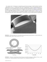
including both time dependent inlet conductance effects and dead volume fractions. The generic positive
displacement pump is illustrated in Figure 8.2.In general, the pumping speed, S
P
, for an intake number
density, n
I
, and an exhaust number density, n
E
(or ℘ corresponding to the pressures, p
I
, and p
E
, since the
process gas temperature is assumed to be constant in the important low pressure pumping range) can be
derived:
S
P
ϭ (1 Ϫ ℘℘
G
Ϫ1
)(1 Ϫ e
Ϫ(C
LI
/V
T,I
f
T
)
β
1

)V
T,I
f
T
Ϫ (℘ Ϫ 1)C
LB
β
2
(8.8)
(1 Ϫ ℘/℘
MAX
)
ᎏᎏ
(1 Ϫ 1/
℘
MAX
)
8-6 MEMS: Applications
© 2006 by Taylor & Francis Group, LLC
In Equation (8.8), ℘ is the pressure ratio p
E
/p
I
ϵ n
E
/n
I
(assuming T
I
ϭ T

E
); C
LI
is the pump’s inlet con-
ductance; V
T,I
is the trapping volume at the inlet; C
LB
is the conductance of the backflow channels
between exhaust and inlet pressures; ℘
G
ϭ V
T,I
/V
T,E
is the geometric trapped volume ratio between inlet
and exit;
β
1
is the fraction of the trapping cycle during which the inlet aperture is exposed; and
β
2
is the
fraction of the cycle during which the backflow channels are exposed to the pressure ratio ℘.
The pumping speed expression of Equation (8.8) applies most directly to a single compression stage.
The backflow conductance is assumed to be constant because the flow is in the “collisionless”flow regime,
which exists in the first few stages of a typical dry pumping system. The inlet conductance for a dry
microscale system will be in the collisionless flow regime at low pressure (say 10
Ϫ2
mbar). The inlet con-

ductance per unit area can increase significantly (amount depends on geometry) for transitional inlet
pressures [Lafferty, 1998; Sone and Itakura, 1990; Sharipov and Seleznev, 1998]. The performance of
macroscale (inlet apertures of several cm and larger) positive displacement pumps at a given inlet pres-
sure will thus benefit from the increased inlet conductance per unit area compared to their reduced scale
counterparts in the important low pressure range of 10
Ϫ3
to 10
Ϫ1
mbar.
The term (1 Ϫ ℘℘
G
Ϫ1
) in Equation (8.8) represents an inefficiency due to a finite dead volume in the
exhaust portion of the cycle. The effect of incomplete trapped volume filling during the open time of the inlet
aperture is represented by (1 Ϫ e
Ϫ(C
LI
/V
T,I
f
T
)
β
1
). The ideal (no inefficiencies) pumping speed is V
T,I
f
T
. The
backflow inefficiency is (℘ Ϫ 1)C

L B
β
2
. The dimensions of all groupings are volume per unit time. As in
all pumps a maximum upflow (S
P,MAX
) can be found by assuming ℘ ϭ 1 in Equation (8.8). Similarly the
Microscale Vacuum Pumps 8-7
4
3
2
1
12
11
10
9
8
7
6
5
Backflow loss
p
I
intake
p
E
exhaust
V
T,E
V

T,I
1 2
Intake from p
I
to V
T,I
at Pressure p
E
/p
G
, partial filling of V
T,I
due to limited inlet time. V
T,I
closed.
2 3
Volume decreases and backflow loss begins.
4 6
Volume continues to decrease to V
T,E
backflow increases,
pressure in V
T,E
> p
E
7
Exhaust of excess pressure from V
T,E
to p
E

8
V
T,E
closed with pressure p
E
7
1
12
Volume expands to V
T,I
pressure drops to p
E
/℘
G
Cycle repeats
℘
G
= V
T,I
/ V
T,E
FIGURE 8.2 Generic positive displacement vacuum pump.
© 2006 by Taylor & Francis Group, LLC
maximum pressure ratio (℘
MAX
) can be obtained from Equation (8.8) by setting S
P
ϭ 0. With some
manipulations Equation (8.8) can be rewritten as:
S

P
ϭ V
T,I
f
T
℘
G
Ϫ1
{1 ϩ (C
LB
β
2
/V
T,I
f
T
)℘
G
Ϫ exp(ϪC
LI
β
1
/V
T,I
f
T
)} (℘
MAX
Ϫ ℘) (8.9)
The relationship between ℘, ℘

MAX
, S
P
, and S
P
,MAX
can be found by setting ℘ ϭ 1 in Equation (8.9).
Substituting back into Equation (8.9) gives the same expression as in Equation (8.7).
For the purposes of this chapter, the upflow of molecules per unit time (N
.
ϭ S
P
n
I
) is a useful measure
of pumping speed. The form of Equation (8.9) has been checked by fitting it successfully to observed
pumping curves (S
P
vs. p
I
) for several positive displacement pumps (using data in Lafferty, 1998) between
inlet pressures of 10
Ϫ2
and 10
0
mbar. This is done by following Equation (8.9) and re-plotting the exper-
imental results using S
P
and (℘
MAX

Ϫ ℘) as the two variables. The variation of inlet conductance with
Kn, C
LI
(Kn), is important in matching Equation (8.9) to the observed pumping performances.
At low inlet pressures, the energy use of positive displacement pumps is dominated by friction losses
due to the relative motion of their mechanical components. Taking the two possibilities of sliding and
viscous friction as limiting cases, the frictional energy losses can be represented as:
Q
.
sf
ϭ u
ෆ
µ
sf
A
s
F
~
N
(8.10a)
for sliding friction; and for viscous friction:
Q
.
µ
ϭ u
ෆ
µ
A
s
(u

ෆ
/h) (8.10b)
Here Q
.
sf
and Q
.
µ
are the powers required to overcome sliding friction and viscous friction respectively. The
coefficients are respectively
µ
sf
and
µ
, A
s
is the effective area involved, F
~
N
is the normal force per unit area,
and u
ෆ
is a representative relative speed of the two surfaces that are in contact for sliding friction or sepa-
rated by a distance, h, for the viscous case. The contribution to viscous friction in clearance channels
exposed to the process gas at low pumping pressures is usually not important, but there may be signifi-
cant viscous contributions from bearings or lubricated sleeves. An estimate of the power use per unit of
upflow can be obtained by combining Equations (8.9) and (8.10) to give (Q
.
/N
.

), with units of power per
molecule per second or energy per molecule.
Consider the geometric scaling to smaller sizes of a “reference system” macroscopic positive displace-
ment vacuum pump. The scaling is described by a scale factor, s
i
, applied to all linear dimensions.
Inevitable manufacturing difficulties when s
i
is very small are put aside for the moment. As a result of the
geometric scaling the operating frequency, f
T,i
, needs to be specified. It is convenient to set f
T,i
ϭ s
i
Ϫ1
f
T,R
,
which keeps the component speeds constant between the reference and scaled versions. This may not be
possible in many cases, another more or less arbitrary condition would be to have f
T,i
ϭ f
T,R
. Using the
scaling factor and Equation (8.9), an expression for the scaled pump upflow, N
.
i
, can be written as a func-
tion of s

i
and values of the pump’s important characteristics at the reference or s
i
ϭ 1 scale (e.g.
V
T,I,i
ϭ s
3
i
V
T,I,R
s
i
Ϫ1
f
T,R
). For the case of f
T,i
ϭ s
i
Ϫ1
f
T,R
:
N
.
i
ϭ n
I
s

3
i
V
T,I,R
s
i
Ϫ1
f
T,R
℘
G
Ϫ1
[1ϩ(s
2
i
C
LB,R
β
2
/s
3
i
V
T,I,R
s
i
Ϫ1
f
T,R
)℘

G
Ϫexp{Ϫ(s
2
i
C
LI,R
β
1
/s
3
i
V
T,I,R
s
i
Ϫ1
f
T,R
)}](℘
MAX
Ϫ ℘) (8.11)
Similarly the scaled version of Equation (8.10b) becomes:
Q
.
µ
,i
ϭ u
ෆ
2
µ

s
2
i
A
S,R
/s
i
h
R
(8.12)
Forming the ratios (Q
.
µ
,i
/Q
.
µ
,R
)/(N
.
i
/N
.
R
) ϵ (Q
.
µ
,i
/N
.

i
)/(Q
.
µ
,R
/N
.
R
) eliminates many of the reference system
characteristics and highlights the scaling. In this case, for the viscous energy dissipation per molecule of
upflow in the scaled system compared to the same quantity in the reference system, a scaling relationship
is obtained:
(Q
.
µ
,i
/N
.
i
)/(Q
.
µ
,R
/N
.
R
) ϭ s
i
Ϫ1
(8.13)

8-8 MEMS: Applications
© 2006 by Taylor & Francis Group, LLC
A summary of the results of this type of scaling analysis applied to positive displacements pumps is
presented in Table 8.2a, along with all the other types of pumps that are considered below. In Table 8.2a,
the performance can be summarized using ℘
MAX
(S
P
ϭ 0) and S
P,MAX
or N
.
MAX
(℘ ϭ 1) in order to elim-
inate ℘ appearing explicitly as a variable in the scaling expressions through the dependency of N
.
on pres-
sure ratio (refer to Equation 8.11).
8.3.2 Kinetic Pumps
Because of their sensitivity to orientation and their potential for contamination, diffusion pumps are not
suitable for MEMS scale vacuum pumps, except possibly for situations permitting fixed installations. The
other major kinetic pumps, turbomolecular and molecular drag, require high rotational speed compo-
nents but are dry; in macroscale versions they can be independent of orientation, at least in time inde-
pendent situations. Only the turbomolecular and molecular drag pumps will be discussed in this chapter.
Bernhardt (1983) developed a simplified model of turbomolecular pumping. Following this descrip-
tion the maximum pumping speed (℘ ϭ 1) of a turbomolecular pumping stage (rotating blade row and
a stator row) can be written as:
S
P,MAX
ϭ A

I
(C
ෆ
Ј/4)(v
c
/C
ෆ
Ј)/[(1/qd
f
) ϩ (v
c
/C
ෆ
Ј)] (8.14)
In Equation (8.14), A
I
is the inlet area to the rotating blade row, v
c
is an average tangential speed of the
blades, q is the trapping probability of the rotating blade row for incoming molecules, besides blade geom-
etry it is a function of (v
c
/C
ෆ
Ј). The term, d
f
, accounts for a reduction in transparency due to blade thick-
ness. It is assumed in Equation (8.14) that the blades are at an angle of 45° to the rotational plane of the
blades. As a convenience, writing v
r

ϭ (v
c
/C
ෆ
Ј), v
r
is similar to but not identical with the Mach number.
The maximum pressure ratio (S
P
ϭ 0) can be written as:
℘
MAX
ϭ e
ξ
v
r
(8.15)
where
ξ
is a constant that depends on blade geometry [Bernhardt, 1983]. Dividing Equation (8.14) by
A
I
(C
ෆ
Ј/4) gives the pumping probability:
α
P,MAX
ϭ v
r
/[(1/qd

f
) ϩ v
r
] (8.16)
Microscale Vacuum Pumps 8-9
TABLE 8.2a Effect of scaling on performance
Type
f
T,i
ϭ s
i
Ϫ
1
f
T,R
(u
–
i
ϭ u
–
R
)
Positive Displacement 1 s
2
i
1 s
i
Ϫ1
s
i

Turbomolecular 1 s
2
i
1 s
i
Ϫ1
s
i
f
T,i
ϭ f
T,R
(u
–
i
ϭ s
i
u
–
R
)
Positive Displacement O
´
[1] to O
´
[s
i
] O
´
[s

3
i
] ϾO
´
[1] ϾO
´
[1] ϾO
´
[1]
Turbomolecular (℘
MAX,R
)
(s
i
Ϫ1)
O
´
[s
4
i
] ϾO
´
[s
i
Ϫ1
] ϾO
´
[s
i
Ϫ1

] ϾO
´
[s
i
Ϫ1
]
(Q
.
/N
.
MAX
)
i
/
(Q
.
/N
.
MAX
)
R
Sputter Ion (inactive and 1 s
2
i
V
D,i
/V
D,R
Ϸ 1 s
i

active gases)
Orbitron Ion Active gases 1 s
2
i
1 s
i
Obitron Ion Inactive gases 1 s
i
1 s
2
i
(ions)
Notes: For the case of f
T,i
ϭ f
T
,R
the expressions that result are sensitive to the particular importance of backflow in each
case. Estimates have been made, using typical values for the losses, of the order of magnitude of these expressions in order
to simplify the presentation. The detailed expressions appear below in Table 8.2b.The scaling of V
P,i
/V
P,R
is assumed to be
as s
3
i
when obtaining the (V
P
/N

.
MAX
)
i
/(V
P
/N
.
MAX
)
R
scaling.
(V
P
/N
.
MAX
)
i
ᎏᎏ
(V
P
/N
.
MAX
)
R
S
P,MAX,i
ᎏ

S
P,MAX,R
℘
MAX,i
ᎏ
℘
MAX,R
(
V
P
/N
.
MAX
)
i
ᎏᎏ
(V
P
/N
.
MAX
)
R
(Q
.
µ
/N
.
MAX
)

i
ᎏᎏ
(Q
.
µ
/N
.
MAX
)
R
(Q
.
sf
/N
.
MAX
)
i
ᎏᎏ
(Q
.
sf
/N
.
MAX
)
R
S
P
,MAX,i

ᎏ
S
P,MAX,R
℘
MAX,i
ᎏ
℘
MAX,R
© 2006 by Taylor & Francis Group, LLC
8-10 MEMS: Applications
TABLE 8.2b Detailed Expressions for Size Scaling with f
T,i
ϭ f
T,R
Type
Positive Displacement
Ά ·
ϫ s
3
i
Ά · Ά · Ά ·
Ά ·
Turbomolecular (℘
MAX,R
)
(s
i
Ϫ1)
s
3

i
Ά · Ά · Ά ·
Notes: The K
I,R
and K
B,R
are associated with the inlet loses and backflow losses respectively (larger K
I,R
leads inlet losses but the larger K
B,R
the more serious the backflow
loss). K
I,R
ϭ C
LI,R
β
1
/V
TI,R
, f
T,R
K
B,R
ϭ C
LB,R
β
2
/V
TI,R
f

T,R
. The symbols are defined in the section on positive displacement pumps.
(q
R
d
f,R
)
Ϫ1
ϩ (s
i
v
c,R
/C
–
Ј)
ᎏᎏᎏ
(q
R
d
f,R
)
Ϫ1
ϩ (v
c,R
/C
–
Ј)
(q
R
d

f,R
)
Ϫ1
ϩ (s
i
v
c,R
/C
–
Ј)
ᎏᎏᎏ
(q
R
d
f,R
)
Ϫ1
ϩ (v
c,R
/C
–
Ј)
(q
R
d
f,R
)
Ϫ1
ϩ (v
c,R

/C
ෆ
Ј)
ᎏᎏᎏ
(q
R
d
f,R
)
Ϫ1
ϩ s
i
(v
c,R
/C
ෆ
Ј)
1 Ϫ exp(ϪK
I,R
) ϩ ℘
G
K
B,R
ᎏᎏᎏᎏ
1 Ϫ exp(Ϫs
i
Ϫ1
K
I,R
) ϩ s

i
Ϫ1
℘
G
K
B,R
1 Ϫ exp(ϪK
I,R
)
ᎏᎏᎏ
1 Ϫ exp(Ϫs
i
Ϫ1
K
I,R
)
1 Ϫ exp(ϪK
I,R
)
ᎏᎏ
1 Ϫ exp(Ϫs
i
Ϫ1
K
I,R
)
1 Ϫ exp(Ϫs
i
Ϫ1
K

I,R
)
ᎏᎏ
1 Ϫ exp(ϪK
I,R
)
1 Ϫ exp(Ϫs
i
Ϫ1
K
I,R
) ϩ s
i
Ϫ1
K
B,R
ᎏᎏᎏᎏ
1 Ϫ exp(ϪK
I,R
) ϩ K
B,R
(Q
.
µ
/N
.
MAX
)
i
ᎏᎏ

(Q
.
µ
/N
.
MAX
)
R
(Q
.
sf
/N
.
MAX
)
i
ᎏᎏ
(Q
.
sf
/N
.
MAX
)
R
S
P,MAX,i
ᎏ
S
P,MAX,R

℘
MAX,i
ᎏ
℘
MAX,R
© 2006 by Taylor & Francis Group, LLC
The ℘
MAX
for turbomolecular stages is generally large (ϾO
´
[10
5
]) for gases other than He and H
2
due to
the exponential expression of Equation (8.15). During operation in a multi-stage pump the stages can be
employed at pressure ratios ℘ ϽϽ ℘
MAX
. Thus, from Equation (8.7) (which also applies to turbomolec-
ular drag stages) the pumping speed approaches S
P,MAX
.
The scaling characteristics of turbomolecular pumps can be derived using Equations (8.14) and (8.15).
It is assumed that the pump blades remain similar during the scaling. The tangential speed (v
c
) will be
written as 2
π
Rf
p

, where R is a characteristic radius of the blade row and f
p
is the rotational frequency in
rps. From Equations (8.14) and (8.15):
(S
P
,MAX
)
i
ϭ s
i
2
A
I
,R
(C
ෆ
Ј/4){[2
π
s
i
R
R
f
P
,i
/C
ෆ
Ј]/[(1/q
i

d
f
,i
) ϩ (2
π
s
i
R
R
f
P
,i
/C
ෆ
Ј)]}
℘
MAX,i
ϭ exp(
ξ
2
π
s
i
R
R
f
P,i
/C
ෆ
Ј) (8.17)

For example, the case of f
P,i
ϭ f
P,R
, d
f,i
ϭ d
f,R
, gives:
ϭ s
i
3
[(1/q
R
d
f,R
) ϩ (v
c,R
/C
ෆ
Ј)]/[(1/q
i
d
f,R
) ϩ (s
i
v
c,R
/C
ෆ

Ј)] (8.18)
℘
MAX,i
ϭ (℘
MAX,R
)
s
i
Ϫ1
(8.19)
For the case of f
P,i
ϭ s
i
Ϫ1
f
P,R
(constant v
c
):
ϭ s
i
2
, ℘
MAX,i
ϭ ℘
MAX,R
(8.20)
Acomplete set of scaling results is presented in Table 8.2a and 8.2b.
8.3.2 Capture Pumps

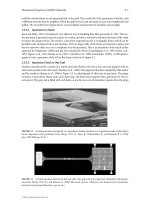
8.3.2.1 Sputter Ion Pumps
The sputter ion pump (SIP) is an option for high vacuum MEMS pumping. The application of simple
scaling approaches to these pumps is difficult; however centimeter scale pumps are already available. The
SIP has a basic configuration illustrated in Figure 8.3. A cold cathode discharge (Penning discharge), self
(S
P,MAX
)
i
ᎏ
(S
P,MAX
)
R
(S
P,MAX
)
i
ᎏ
(S
P,MAX
)
R
Microscale Vacuum Pumps 8-11
S
S
S
S
B
e
e

S
S
S
S
Ions sputter cathode and are
permanently buried on
periphery of both cathodes.
Cathode
Pumping is through
spaces between
cathodes
and anode
Cylindrical anode
Cathode
Active neutrals are
adsorbed and
sputtered material
deposited on anode's
inner wall.
V
d
+
+
+
+
+
+
+
.
.

.
FIGURE 8.3 Figure Sputter ion pump schematic.
© 2006 by Taylor & Francis Group, LLC
maintained by a several thousand volt potential difference and an externally imposed magnetic field that
restricts the loss of discharge electrons, causes ions created in the discharge by electron-neutral collisions
to bombard the cathodes. The energetic ions (with energy some fraction of the driving potential) both
sputter cathode material (usually Ti) and imbed themselves in the cathodes. Sputtered material deposits
on the anode and portions of the opposing cathodes. The freshly deposited material acts as a continu-
ously refreshed adsorption pumping surface for “active”gases (most things other than the noble gases and
hydrocarbons). Small (down to an 8mm diameter anode cylinder and a cathode separation of 3.6 cm)
pumps have been studied theoretically by Suetsugu (1993). His results compare reasonably well to exper-
imental results for the particular case of a 1.5 cm diameter anode. For a discharge voltage of 3000 V, a
magnetic field strength of 0.3 T and a 0.8 cm diameter anode a pumping speed of slightly greater than
0.5 l/s is predicted at 10
Ϫ8
Torr. For these conditions the discharge is operating in the high magnetic field
(HMF) mode, which results in a maximum pumping speed. The pumping speed increases slowly as
pressure increases.
SIP’s have a finite but relatively long life; they may be useful when ultra high vacuums are required in
small scale systems. Their scaling to true MEMS sizes is uncertain because they require several thousand
volts to operate reasonably effectively (ion impact energies approaching 1000 V are required for efficient
sputtering and rare gas ion burial). The description of SIP operation developed by Suetsugu (1993) can
be used to provide a scaling expression (that needs to be employed cautiously). The power used by the
discharge can be obtained knowing the applied potential difference, V
D
, and the ion current, I
ion
. Suetsugu
(1993) gives for the pumping speed:
S

P
ϭ (K
G
q
η
I
ion
)/(3.3 ϫ 10
19
)ep
I
(8.21)
where p
I
is the pressure in Torr,
η
is the sputtering coefficient of cathode material due to the impact of ener-
getic ions, and q is the sticking coefficient for active gases on the sputtered material. The charge on an elec-
tron is e,K
G
is a non-dimensional geometric parameter derived from the electrode configuration that remains
constant with geometric scaling. An expression for the power required per pumped molecule becomes:
(Q
.
/N
.
)
i
ϭ (V
D

I
ion
)
i
/[{(K
G
q
η
I
ion
)/((3.3 ϫ 10
19
)ep
I
)}
i
{10
Ϫ3
n
I
}] (8.22)
and
(Q
.
/N
.
)
i
/(Q
.

/N
.
)
R
ϭ V
D,i
/V
D,R
(8.23)
This assumes q
i
ϭ q
R
,
η
i
ϭ
η
R
.
The scaling expression for pumping speed becomes:
S
P,i
/S
P,R
ϵ S
P,MAX,i
/S
P,MAX,R
ϭ (I

ion
)
i
/(I
ion
)
R
(8.24)
where the S
P,MAX
is employed to be consistent with the previous useage for other pumps, although the
Equation (8.7) relationship does not really apply in this case.
The ion current is obtained by an iterative numerical solution involving the number density of trapped
electrons [Suetsugu, 1993]. The scaling expression for Q
.
/N
.
in Equation (8.23) is particularly simple
because the ion currents cancel. The scaling represented by Equation (8.23) appears reasonably valid pro-
viding
η
remains relatively constant, which implies that the ion energy should be relatively constant. Ion
burial in the cathodes, which is the mechanism by which SIPs pump rare gases, is not discussed in detail
in this chapter but can be considered within the framework of Suetsugu’s analysis. Scaling results are
summarized in Table 8.2a.
8.3.2.2 Orbitron Ion Pump
The orbitron ion pump [Douglas, 1965; Denison, 1967; Bills, 1967] was developed based on an electro-
static electron trap best known for application in ion pressure gauges. A sketch is presented in Figure 8.4.
8-12 MEMS: Applications
© 2006 by Taylor & Francis Group, LLC

Injected electrons orbit an anode, the triode version illustrated in Figure 8.4 [Denison, 1967; Bills, 1967]
has an independent sublimator that provides a continuous active getter (Ti) coating of the ion collector.
The getter permits active gas pumping as well as permanent burial of rare gas and other ions that are
accelerated out of the trap through the cathode mesh by the radial electric fields. Initial work on reduc-
ing the size of an orbitron to MEMS scales has recently been reported by Wilcox et al. (1999).
For a given geometry and potential difference between the anode and cathode mesh the cylindrical
capacitor represented by the trap geometry has a limiting maximum net negative charge of orbiting elec-
trons. The corresponding ionization rate in the trap can be written as:
N
.
MAXions
ϭ (8.25)
where X is the fraction of the maximum charge that permits stable electron orbits (less than 0.5), V
D
is the applied potential difference, m
e
is the electron mass,
ε
0
is the permittivity of free space, Ω
I
is the
electron-neutral ionization cross-section, L is the trap’s length, r
2
and r
1
are the radii of the trap’s cathode
and anode respectively (Figure 8.4).
The orbitron’s noble gas pumping speed and the trap’s volume can be scaled based on the expression
for ionization rate in Equation (8.25):

ϭ s
i
; ϭ s
i
2
(8.26)
Note that this is favorable scaling.
The sublimator’s scaling, assuming the temperature of the sublimating getter is constant, can be writ-
ten for neutrals and ions as:
ϭ 1; ϭ 1 (8.27)
(Q
.
ion
/N
.
MAXions
)
i
ᎏᎏ
(Q
.
ion
/N
.
MAXions
)
R
(Q
.
s

/N
.
MAXneut
)
i
ᎏᎏ
(Q
.
s
/N
.
MAXneut
)
R
⍀
I,i
(V
D
)
i
3/2
ᎏᎏ
⍀
I,R
(V
D
)
R
3/2
(V

P
/N
.
MAXions
)
i
ᎏᎏ
(V
P
/N
.
MAXions
)
R
⍀
i
(V
D
3/2
)
i
ᎏᎏ
⍀
R
(V
D
3/2
)
R
(S

P,MAXions
)
i
ᎏᎏ
(S
P,MAXions
)
R
2X
πε
0
V
D
3/2
Ω
I
Ln
g
ᎏᎏ
(em
e
)
1/2
ln(r
2
/r
1
)
3/2
Microscale Vacuum Pumps 8-13

L
Sublimator, getter deposited on
collector
Anode
Ion pump
Sublimator
Ions created in
trap accelerate
radially through
cathode to
collector.
Active neutrals
and ions pumped
by getter from
sublimator.
Grids on plates at ends of traps to reflect
electrons and maximize trap efficiency.
Electron emitter
Collector, biased negative with
respect to cathode to enable
efficient ion burial in collector.
e
−
, at about 100 eV
Trapped
electrons
Grid
cathode
r
1

r
2
+
+
FIGURE 8.4 Orbitron pump schematic.
© 2006 by Taylor & Francis Group, LLC
8.4 Pump-Down and Ultimate Pressures for
MEMS Vacuum Systems
What is the consequence of size scaling a vacuum system? Consider an elementary system made up of a
pump and a vacuum chamber of volume V
c
and surface area A
sc
. The pump is modeled by writing the
pumping speed as:
S
P,i
ϭ {A
I,P
(C
ෆ
Ј/4)
α
P
}
i
(8.28)
where A
I,P
is the area of the pump’s inlet aperture from the chamber and

α
P
is the probability that
once through the aperture a molecule will be pumped. For a geometrically similar size change
S
P,i
ϭ s
2
i
(
α
P,i
/
α
P,R
)S
P,R
, and the pumping speed per unit surface area of the vacuum chamber is:
(S
P
/A
sc
)
i
/(S
P
/A
sc
)
R

ϭ
α
P,i
/
α
P,R
(8.29)
Assuming equal outgassing rates per unit area for the reference and scaled systems, the ultimate system
pressure will only depend on the pumping probability ratio
α
P,i
/
α
P,R
. The pump-down time for the
system can be measured using the ratio S
P
/V
c
ϭ
τ
P
:
τ
P,i
/
τ
P,R
ϭ s
i

(
α
P,R
/
α
P,i
) (8.30)
For geometric scaling and the same outgassing rates a MEMS system will have a significantly shorter
pump-down time assuming
α
P,i
/
α
P,R
can be kept near one.
In practice MEMS scale vacuum systems are likely to have pump apertures relatively much larger than
their macroscopic counterparts. The economic deterrent to having large aperture pumps that exists at
macroscales does not apply at MEMS scale. At MEMS scales it appears that technical issues associated
with pump construction will favor making the pumps as large as possible. Consequently, relatively large
pump apertures with areas about the same as the cross section of the pumped volume are anticipated.
8.5 Operating Pressures and N
.
Requirements in
MEMS Instruments
The selection of vacuum pumps for MEMS instruments and processes will depend on operating pressure
and N
.
requirements. Since this can be determined reliably only when the task, instrument, and detector
or a particular process have been specified, it is virtually impossible to discuss significant general size scal-
ing tendencies. For example, there has been speculation [R.M. Young, 1999] that a MEMS mass spectrom-

eter sampling instrument might operate at upper pressures specified by keeping the Knudsen number
based on the quadrupole length constant compared to similar macroscale instruments. This can typically
lead to tolerable upper operating pressures for microscale instruments of 10
Ϫ3
to 10
Ϫ2
mbar, depending
on the scaling factor (see also Ferran and Boumsellek, 1996). On the other hand the default response of
many mass spectroscopists is 10
Ϫ5
mTorr, independent of scaling. Vargo (2000) based N
.
requirements for
a miniaturized sampling mass spectrometer on the goal of replacing the entire volume of gas in the
instrument (30 cm
3
in Vargo’s case) every second at an operating pressure of 10
Ϫ4
mTorr, giving
N
.
ϭ 1.4 ϫ 10
14
molecules/s. A point to remember is that for a constant Kn system the equilibrium quantity
of adsorbed gas in the system increases compared to unadsorbed gas as the s
i
decreases [Muntz, 1999].
A careful consideration of the operating pressure and N
.
requirements for a particular situation is

important, but impossible within the confines of this chapter. Because of the difficulty in supplying
volume and power compatible microscale vacuum systems, it will be important for overall system design
to define operating conditions that are based on real needs.
8-14 MEMS: Applications
© 2006 by Taylor & Francis Group, LLC
8.6 Summary of Scaling Results
The scaling analyses previously outlined have been applied to several pump types, with the results appear-
ing in Table 8.2a and b. The operating frequencies were selected to give two extremes: maintaining a con-
stant average speed u
ෆ
i
ϭ u
ෆ
R
(tangential for rotating devices or linear for reciprocating), by using the
frequency scaling, f
T,i
ϭ s
i
Ϫ1
f
T,R
; or maintaining a constant frequency, f
T,i
ϭ f
T,R
, resulting in u
ෆ
i
ϭ s

i
u
ෆ
R
. Two
alternative types of frictional drag — sliding and viscous — have been included, again as extremes of the
likely possibilities.
The scaling expressions for the case u
ෆ
i
ϭ u
ෆ
R
are simple when normalized by their respective reference
scale values. For the second case where u
ෆ
i
ϭ s
i
u
ෆ
R
, the expressions are more complex and the results depend
on the relative magnitude of the quantities K
I,R
, K
B,R
, q
R
d

f,R
, etc. (Table 8.2(b)). For the cases involving
more complex expressions order of magnitude estimates of the scaling based on typical pump character-
istics have been included in Table 8.2(a).
The sputter ion pumps have been included assuming that permanent magnets provide the required
field strengths. Note that the mesoscale SIP performance presented in Figure 8.1 and Table 8.1 is for HMF
operation.
To put the scaling results in Table 8.2 in perspective, remember that they are for geometrically accurate
scale reductions. It is assumed that the relative dimensional accuracy of the components is the same in
the reduced scale realization as in the reference macroscopic pumps. This is a very idealized assumption.
The dimensional accuracy that can currently be attained in micromechanical parts as a function of size
is illustrated in Figure 8.5 (derived in part from Madou, 1997). It is clear from Figure 8.5 that the scaling
results of Table 8.2 may be very optimistic if true MEMS scale pumps (component sizes 100 µm or less)
are required. On the other hand the scalings do represent the best scaled performances that could be
expected and are a useful guide. Note from Figure 8.5 that the smallest fractional tolerances can be
achieved by precision machining techniques for approximately 1 cm size components. As a result,
mesoscale pumps may be possible from a tolerance (although perhaps not economic) perspective using
precision machining techniques.
Microscale Vacuum Pumps 8-15
Tolerances less than about 0.01%
achieved by precision machining
techniques.
Typical tolerances
for a roots blower
Tolerances for a
turbomolecular pump.
From Madou (1997)
Linear dimension (m)
Relative tolerance (%)
10

−5
10
−4
10
−3
10
−2
10
−1
10
−1
10
−2
10
−3
10
−4
10
−5
10
−6
10
−7
10
−8
10
0
10
1
10

2
10
2
10
1
10
0
FIGURE 8.5 Dimensional accuracy of manufactured components as a function of size. (After Madou, M. [1997]
Fundamentals of Microfabrication, CRC Press, Boca Raton, Florida.)
© 2006 by Taylor & Francis Group, LLC
Several points should be noted from Table 8.2.For the case of u
ෆ
i
ϭ u
ෆ
R
, the ideal scalings to small sizes
are reasonable (remember s
i
will range between 10
Ϫ1
and 10
Ϫ4
). In the case of viscous friction losses, the
energy use per molecule of upflow becomes large at small scales (increases as s
i
Ϫ
1
) while the pump vol-
ume per unit upflow decreases as s

i
decreases. For the case of positive displacement pumps and u
ෆ
i
ϭ s
i
u
ෆ
R
,
the energy use per molecule of upflow scales satisfactorily, but upflow scales as s
i
3
so that the volume scal-
ing is of O
´
[1] rather than the s
i
Ϫ
1
for the u
ෆ
i
ϭ u
ෆ
R
case. The ℘
MAX
scaling to small scales for u
ෆ

i
ϭ s
i
u
ෆ
R
is a
disaster for turbomolecular pumps. Also the upflow, energy, and pump volume all scale badly for the tur-
bomolecular pump with u
ෆ
i
ϭ s
i
u
ෆ
R
. These scalings are all a result of the trapping coefficient q ϳ s
i
for low
peripheral speeds. Although not explicitly included, molecular drag pumps can be expected to scale sim-
ilarly to the turbomolecular pump. For positive displacement pumps the pressure ratio scales well if there
are no losses but can scale as badly as s
i
depending on specific pump characteristics. For the cases where
the pressure ratio scales badly, more pump stages would be required for a given task, leading to larger
pumps as indicated by the Ͼ symbol in the energy use and pump volume per unit upflow columns.
The sputter ion pump scales well to smaller sizes. The major concern for microscales will be the fun-
damental requirement for relatively high voltages. Also, thermal control will be difficult as it is compli-
cated by the need for high field strengths (0.5–1 T) using co-located permanent magnets.
The orbitron ion pump scales well to smaller sizes but unfortunately as seen in Figure 8.1 and Table

8.1 begins with a very poor performance as measured by Q
.
/N
.
.
Generally, for the positive displacement and turbomolecular pumps, the idealized geometric scaling
results in Table 8.2 demonstrate that there is a mixed bag of possibilities, ranging from decreased per-
formance to maintaining performance, with a few cases showing improvement on macroscale perform-
ance by going to smaller scales. From a vacuum pump perspective with ideal scaling there is little to no
advantage based on performance to go to small scales, except for the ion pumps.
The actual performance of small-scale pumps is likely to be significantly poorer than the idealized scal-
ing results shown in Table 8.2. For instance it is very difficult to attain the high rotational speeds neces-
sary to satisfy the u
ෆ
i
ϭ u
ෆ
R
requirements in MEMS scale devices; on the other hand, recent progress in air
bearing technology has been reported for mesoscale gas turbine wheels [Fréchette et al., 2000]. Mesoscale
sputter ion pumps have been operated and the investigation of orbitron scaling is just beginning.
Whether either can be scaled to true MEMS sizes is unclear, but they may be the only alternative for
achieving high vacuum with MEMS pumps.
Keeping the preceding comments in mind it is useful to re-visit the macroscale vacuum pump
performances reviewed in Figure 8.1. Consider a typical energy requirement from Figure 8.1 of
3 ϫ 10
Ϫ15
W/molecule of upflow for macroscale systems; assume that this can be maintained at mesoscales
to pump through a pressure ratio of 10
6

(10
Ϫ3
mbar to 1 bar). A typical upflow, assuming a 3 cm
3
volume
at 10
Ϫ3
mbar is changed every second, is 1.1 ϫ 10
14
molecules/s and the required energy is 0.33 W. This is
somewhat high but tolerable for a mesoscale system. However, with the expected degradation of the per-
formance of complex macroscale pumps at meso- and microscales, it is clear that it is important to search
for alternative, unconventional pumping technologies that will be both buildable and operate efficiently
at small scales.
8.7 Alternative Pump Technologies
The previous section on scaling indicates that searching for appropriate alternative technologies as a basis
for MEMS vacuum pumps is necessary. There has been some effort in this regard during the past decade.
In 1993, Muntz, Pham-Van-Diep, and Shiflett hypothesized that the rarefied gas dynamic phenomenon
of thermal transpiration might be particularly well suited for MEMS scale vacuum pumps. Thermal tran-
spiration is the application of a more general phenomenon — thermal creep — that can be used to pro-
vide a pumping action in flow channels for Knudsen numbers ranging from very large to about 0.05. The
observation resulted in a publication [Pham-Van-Diep, 1995], which led to the construction of a prototype
micromechanical pump stage by Vargo (2000) and Vargo et al. (1999).A 15-stage radiantly driven Knudsen
Compressor along with a complete cascade performance model has been developed recently by M. Young
8-16 MEMS: Applications
© 2006 by Taylor & Francis Group, LLC
(2004), Young et al., 2004. A MEMS thermal transpiration pump has also been proposed by R.M. Young
(1999). There is one fundamental problem with thermal transpiration or thermal creep pumps: they are
staged devices that require part of each stage to have a minimum size corresponding to a dimension greater
than about 0.2 molecular mean free paths (

λ
) in the pumped gas.At 1mTorr (1.32 ϫ 10
Ϫ
3
mbar)
λ
Ϸ 0.05m
in air, resulting in required passages no smaller than about 1 cm. Thus, at low inlet pressures the pumps
can be unacceptably large for MEMS applications. This issue has been discussed by Han et al., 2004.
An interestingly different version of a thermal creep pump has been suggested by Sone and his
co-workers [Sone et al., 1996; Aoki et al., 2000; Sone and Sugimoto, 2003], although it also has a low pres-
sure use limit similar to the one mentioned previously.
Another alternative, the accommodation pump, which is superficially similar to thermal transpiration
pumps but based on a different physical phenomenon, has been investigated [Hobson, 1970]. It can in
principle be used to provide pumping at arbitrarily low pressures without minimum size restrictions.
8.7.1 Outline of Thermal Transpiration Pumping
Two containers, one with a gas at temperature T
L
and one at T
H
are separated by a thin diaphragm of area
A
i
in which there are single or multiple apertures that each have an area A
a
and a size
͙
A
ෆ
a

ෆ
ϽϽ
λ
L
or
λ
H
(Figure 8.6). The number of molecules hitting a surface per unit time per unit area in a gas is nC
ෆ
Ј/4. In
Figure 8.6 this means that there are (n
L
C
ෆ
Ј
L
/4) molecules passing from cold to hot through an aperture.
Similarly, there are (n
H
C
ෆ
Ј
H
/4)A
a
molecules per unit time passing from hot to cold into the cold chamber.
Assume m is the same for the molecules in both chambers and assume that the inlet and outlet are
adjusted so that p
L
ϭ p

H
. Under these circumstances the net number flow of molecules from cold to hot
is, with the help of the equation of state:
N
.
MAX
ϭ A
a
(2
π
mk)
Ϫ1/2
p
L
[T
H
1/2
Ϫ T
L
1/2
]/(T
L
T
H
)
1/2
(8.31)
If on the other hand there is no net flow:
(p
H

/p
L
)
N
.
ϭ0
ϭ ℘
MAX
ϭ (T
H
/T
L
)
1/2
(8.32)
For p
H
between p
L
and p
L
(T
H
/T
L
)
1/2
there will be both a pressure increase and a net flow, which is the
necessary condition for a pump! This effect is known as thermal transpiration. If there are Γ apertures
the total upflow of molecules is:

N
.
ϭ ΓA
a
(2
π
mk)
Ϫ1/2
[p
L
/T
L
1/2
Ϫ p
H
/T
H
1/2
] (8.33)
If the hot gas at T
H
is allowedtocool and sent to another stage as indicated in Figure 8.7, for the condi-
tion
λ
ϽϽ
͙
A
ෆ
j
ෆ

, where A
j
is the stage area (but also
λ
ϾϾ
͙
A
ෆ
aj
ෆ
) the pressure p
L,jϩ1
ϭ p
H,j
. Thus a cascade of
stages with net upflow is a pump with no net temperature increase over the pump cascade. This cascade
Microscale Vacuum Pumps 8-17
n
L
T
L
p
L
n
H
T
H
p
H
Flow (N)

Flow (N)
Aperture area, A
a
Thin membrane
Containers cross sectional area, A
FIGURE 8.6 Elementary single stage of a thermal transpiration compressor.
© 2006 by Taylor & Francis Group, LLC
of thermal transpiration pump stages has no moving parts and no close tolerances between shrouds and
impellars, so it is an ideal candidate for a MEMS pump. However, the compressor stages sketched in
Figure 8.7 have a serious problem. The thin films containing the apertures are not practical in most appli-
cations because of heat transfer considerations. A more practical stage is shown in Figure 8.8 where the
thin membrane has been replaced by a bundle of capillary tubes. The temperature and pressure profiles
in the stage are also illustrated in Figure 8.8 along with nomenclature that will be used below.
The stage configuration in Figure 8.8 can be put in a cascade (Figure 8.7) to form a pump as proposed
by Pham-Van-Diep et al. (1995). It was called a Knudsen Compressor after original work by Knudsen,
(1910a and b). Several investigations implementing thermal transpiration in macroscale pumps have
been made over the years [Baum, 1957; Turner, 1966; Hopfinger, 1969; Orner, 1970], but with no result
beyond initial analysis and laboratory experimental studies. For the Knudsen Compressor a performance
analysis was presented for the case of collisionless flow in the capillaries and continuum flow in the con-
nectors [Pham-van-Diep, 1995]. Energy requirements per molecule of upflow (Q
.
/N
.
) were estimated.
Recently Muntz and several collaborators [Muntz et al., 1998; Vargo, 2000; Muntz et al., 2002; Han et al.,
2004] have extended the analysis to situations where the flow in both the capillaries and connector sec-
tion can be in the transitional flow regime (10 Ͼ Kn Ͼ 0.05). An initial look at the minimization of cas-
cade energy consumption and volume has been conducted by searching for minimums in Q
.
/N

.
and V
p
/N
.
[Muntz, 1998; Vargo, 2000; Muntz et al., 2002]. Based on these studies a preprototype micromechanical
Knudsen Compressor stage has been constructed and tested [Vargo, 2000; Vargo and Muntz, 1996; Vargo
and Muntz, 1998]. Additional optimization analysis has been recently completed to provide designs for
Knudsen Compressors operating at different pressure ratio-gas upflow conditions [Young et al., 2001;
Young et al., 2003; Young et al., 2004; Young, 2004].
For transitional flow in a capillary tube with a longitudinal temperature gradient imposed on the tube’s
wall, flow is driven from the cold to hot ends as illustrated in Figure 8.9. The increased pressure at the hot end
drives the return flow. For small temperature differences and thus small pressure increases, the Boltzmann
equation can be linearized and results obtained for the flow through a cylindrical capillary driven by small
wall temperature gradients [Sone and Itakura, 1990; Loyalka and Hamoodi, 1990; Loyalka and Hickey, 1991].
The definition of the flow coefficients (Q
T
and Q
P
) are implied in the following expression [Sone, 1968]:
M
.
ϭ p
AVG
(2(k/m)T
AVG
)
Ϫ1/2
A
΄

Q
T
Ϫ Q
p
΅
(8.34)
Here A is the cross-sectional area of the capillary, L
r
its radius, Q
P
is the backflow due to the pressure
increase, and Q
T
is the thermally driven upflow near the walls. The sum determines the net mass flow
dp
ᎏ
dx
L
r
ᎏ
p
AVG
dT
ᎏ
dx
L
r
ᎏ
T
AVG

8-18 MEMS: Applications
N
•
T
L, l−1
T
L, l +1
P
l +1
P
l−1
P
l
(P
l
)
EFF
(P
l −1
)
EFF
(P
l−2
)
EFF
T
L, l
T
H, l
T

H, l −1
T
H, l+1
N
•
Membrane, A
l +1
;
Γ
l +1
apertures of
area A
a,l +1
Membrane area, A
l −1
;
Γ
l−1
apertures of
area A
a,l −1
Membrane, A
l
;
Γ
l
apertures of
area A
a,l
(l − 1)th stage (l + 1)th stagelth stage

FIGURE 8.7 Cascade of thermal transpiration stages to form a Knudsen Compressor (the pressure difference,
(p
ഞ
)
EFF
Ϫ p
ഞ
,drives the flow through the connector as illustrated in Figure 8.8).
© 2006 by Taylor & Francis Group, LLC
through the tube from cold to hot. For large Kn(ϭ
λ
/L
r
) the M
.
ϭ 0 pressure increase provided by a tube
is p
H
/p
C
ϭ Q
T
/Q
P
ϭ (T
H
/T
C
)
1/2

, identical to the aperture case discussed earlier. In the large Kn case the
backflow and upflow completely mingle over the entire tube cross-section. For transitional Kn’s
the upflow is confined near the wall in a layer on the order of
λ
thick, as illustrated in Figure 8.9.
The values of Q
T
and Q
P
vary markedly throughout the transitional flow regime as shown in Figure
8.10. The details of their functional variation as well as the ratio Q
T
/Q
P
are important to any pump using
thermal transpiration. Their roles are best illustrated by the expression for pumping speed and pressure
ratio of a Knudsen Compressor’s j’th stage [Muntz et al., 1998; Muntz et al., 2002]:
S
P,j
ϭ
π
1/2
(1 Ϫ
κ
j
)
Έ Έ΄
Ϫ
΅
j

΄
ϩ
΅
j
Ϫ1
(C
A
)
j
(8.35)
In Equation (8.35) the
κ
j
is a parameter that sets the fraction of the M
.
ϭ 0 pressure rise that is realized in
a finite upflow situation. The pressure ratio for the stage, assuming |∆T/T
AVG
| ϾϾ 1 is:
℘
j
ϭ 1 ϩ
κ
j
ΆΈ Έ΄
Ϫ
΅
j
·
(8.36)

Q
T,C
ᎏ
Q
P,C
Q
T
ᎏ
Q
P
⌬T
ᎏ
T
AVG
L
X
/L
R
ᎏᎏ
F
C
(A
c
/A)Q
P
L
x
/L
r
ᎏ

FQ
P
Q
T,C
ᎏ
Q
P,C
Q
T
ᎏ
Q
P
⌬T
ᎏ
T
AVG
Microscale Vacuum Pumps 8-19
x
x
∆T
l
2
∆T
l
2
T
P
p
l
Capillary

radius, L
r
, l
T
L
,l
T
H,l
T
L,l +1
L
x,l
L
x,l
lth stage(l −1)th stage (l −1)th stage
Gas flow
Connector sectionCapillary section
T
AVG
(p
l −1
)
EFF

l
∆p
l,l
L
R,l
∆p

C,l
(∆p
l
)
T
(p
l
)
EFF
FIGURE 8.8 Capillary tube assembly as a model of a practical Knudsen Compressor.
© 2006 by Taylor & Francis Group, LLC
Other symbols in Equations (8.35) and (8.36) are: |∆T|, the temperature change across both the capillary
section and the connector section; F, the fraction of the capillary section’s area; A
j
; which corresponds to
the open area of the capillary tubes; F
C
, the fraction of the connector section’s area; and A
C,j
, which is open
(usually F
C,j
ϭ 1). The dimensions L
x, j
, L
X,j
, L
r, j
, and L
R,j

are defined in Figure 8.8.
From Equation (8.36), if
κ
j
ϭ 0, then ℘
j
ϭ 1. The corresponding maximum upflow is obtained by
substituting
κ
j
ϭ 0 into Equation (8.35) to give (S
P,MAX
)
j
. The result is:
S
P,j
/(S
P,MAX
)
j
ϭ (1 Ϫ
κ
j
) (8.37)
8-20 MEMS: Applications
λ
λ
x
Tube wall

Slow return flow
p =p
L
Cold
T
L
p =p
H
Hot
T
H
Thermal
creep
flow
Thermal
creep
flow
dT
dx
=
∆
T
∆x
=
T
H
−T
L
x
H

−
x
L
Wall temperature gradent
FIGURE 8.9 Transitional flow configuration in a capillary tube.
0.8
0.7
0.6
0.5
0.4
0.3
0.2
0.1
0
1000 100 10 1 0.1 0.01
5
0
10
15
20
25
30
Q
p
Q
T
, Q
T
/Q
p

Q
T
/Q
p
Q
T
Q
p
Cylindrical tubes
Kn
FIGURE 8.10 Transitional flow coefficients as a function of Knudsen number (Kn ϭ
λ
/L
r
) for cylindrical capillar-
ies. (After Vargo, S.E. [2000] The Development of the MEMS Knudsen Compressor as a Low Power Vacuum Pump
for Portable and In Situ Instruments, Ph.D. Thesis, University of Southern California, Los Angeles.]
© 2006 by Taylor & Francis Group, LLC
which can be combined with the expression for ℘
j,MAX,j
(using
κ
j
ϭ 1 in Equation [(8.35]) to give the
familiar relationship for a vacuum pumping system (Equation [8.7]) between S
P,j
, S
P,MAX,j
, ℘
j

and ℘
MAX,j
.
The expression for pumping speed in Equation (8.35) can also be used to compute the pumping prob-
ability,
α
P,j
, where from Equation (8.5)
α
P,j
ϭ S
p,j
/C
A,j
. Using Equations (8.35) and (8.36) and remembering
that N
.
j
ϭ S
P, j
n
I,j
, where n
I,j
is the number density at the inlet to the stage, cascade performance calcula-
tions can be accomplished. The approach is presented in detail by Muntz et al. (2002). The results of
several cascade simulations are given by Vargo (2000). As shown by Muntz, the majority of the energy
required is the thermal conduction loss across the capillary tube bundle. The physical realization of the
capillary section of a Knudsen Compressor is frequently not a bundle of capillary tubes, but rather a
porous membrane. Nevertheless the theoretical behavior based on “equivalent” capillary tubes appears to

be consistent with the results obtained experimentally [Vargo’s Ph.D. Thesis, Vargo 2000, and the discus-
sions presented therein].
Selected results of micro-, meso-, and macroscale pump cascade simulations reported by Vargo (2000)
are plotted in Figure 8.11 and presented in Table 8.3.Note that all the Knudsen Compressor cascade
results are from simulations; a micromechanical cascade has yet to be constructed although several
mesoscale stages have been operated in series [Vargo, 1996]. More recently, a 15-stage conventionally
machined radiantly driven Knudsen Compressor has been demonstrated by Young (2004). In his thesis,
Vargo (2000) describes the construction of a laboratory prototype micromechanical Knudsen
Compressor stage and the experimental results. A scheme for constructing a cascade is also presented,
along with predicted energy requirements, but this has yet to be built and tested. The Knudsen
Compressor performance presented in Figure 8.11 is based on a significant body of preliminary work, but
has been only partially demonstrated experimentally [Young, 2004; Young et al., 2004]. The Figure 8.11
results are for varying initial pressures p
I
and pumping to 1 atm, the detailed conditions are presented in
Table 8.3. In MEMS devices pressures below 10 mTorr extract a significant energy penalty, tending to preclude
Microscale Vacuum Pumps 8-21
0.1 1 10
100
p
I
mTorr
10
−11
10
−12
10
−13
10
−

14
10
−15
10
−16
10
−17
10
−
11
10
−12
10
−13
10
−14
10
−15
10
−16
10
−17
V
p
/N
•
V
p
/N
MIcro /Meso

•
V
p
/N
Macro
•
Q/ N
•
•
Q/ N
MIcro /Meso
•
•
Q/ N
Macro
•
•
FIGURE 8.11 Simulation results for several macro- and microscale pumping tasks from p
I
to p
E
ϭ 1 atm using
Knudsen compressors. (After results from Table 3 of Vargo, S.E. [2000] The Development of the MEMS Knudsen
Compressor as a Low Power Vacuum Pump for Portable and In Situ Instruments, Ph.D. Thesis, University of Southern
California, Los Angeles.]
© 2006 by Taylor & Francis Group, LLC
Knudsen Compressor applications to lower pressures at MEMS scale. This restriction, however, depends
on the N
.
that is required. The energy penalty originates from the difficulty in reaching effectively contin-

uum flow in the connector section for a reasonable size. Note that the macroscale simulations presented
in Figure 8.11 give efficient pumping to significantly lower p
I
(higher ℘).
The size scaling of Knudsen Compressors at low inlet pressures is dominated by the ratio L
R
/L
r
, that
can be achieved in the early stages of a particular design. The ratio L
R
/L
r
, determines the Knudsen num-
ber ratio which in turn determines the Q
T
/Q
P
ratio (Figure 8.10). By referring to Equation (8.36)
the effects on the stage ℘
j
are immediately clear. In the limit of L
R
/L
r
→ 1, ℘ ϭ 1. For L
R
/L
r
ϾϾ 1,

Q
T,C
/Q
P,C
ϽϽ 1 and ℘
j
reaches a maximum value that depends only on
κ
j
and |∆T/T
AVG
|.
The minimization of a Knudsen Compressor cascade’s energy requirement depends on a number of
important parameters describing individual stage configurations. The results reported by Vargo (2000)
are only a beginning attempt at optimizing Knudsen Compressor performance (there are extended dis-
cussions of optimization issues in Muntz et al.’s report [1998, 2002]). The predicted Knudsen Compressor
Performance presented in Figure 8.11 is quite promising. Generally, as illustrated in Figure 8.12, the
energy requirement for the micro-mesoscale version is at least an order of magnitude better than
macroscale, positive displacement mechanical backing pumps. It also appears very competitive with the
macroscale molecular drag kinetic backing pumps used in conjunction with turbomolecular pumps.
Another MEMS thermal transpiration compressor has been proposed by R.M. Young (1999). Its con-
figuration is different from the Knudsen Compressor, relying on temperature gradients established in the
gas rather than along a wall. No experimental or theoretical analysis of the flow or pressure rise charac-
teristics of this configuration has been reported. There are theoretical reasons to believe that the flow
effects induced by thermal gradients in a gas are significantly smaller than the effects supported by wall
thermal gradients [Cercignani, 2000].
8.7.2 Accommodation Pumping
In 1970 Hobson introduced the idea of high vacuum pumping by employing a characteristic of surface
scattering that had been observed in molecular beam experiments (c.f. the review by Smith and Saltzburg,
1964). For some surfaces that give quasi specular reflection under controlled conditions, when the beam

temperature differs from the surface temperature, the quasi specular scattering lobe moves towards the
surface normal for cold beams striking hot surfaces. For hot beams striking cold surfaces, the lobe moves
away from the normal. Hobson’s initial study was followed in short order by several investigations adopt-
ing the same approach [Hobson and Pye, 1972; Hobson and Salzman, 2000; Doetsch and Ryce, 1972;
Baker et al., 1973]. Other investigators, relying on the same phenomenon, have used different
8-22 MEMS: Applications
TABLE 8.3 Results of Simulations of Micro/meso and Macro Scale Knudsen
Compressors for Several Pumping Tasks (from Vargo, 2000)
p
I
(mTorr) p
E
(mTorr) Q
.
/N
.
W/(#/s) V
P
/N
.
cm
3
/(#/s) ℘
Micro/Meso scale (from Vargo Tables 3, 4 and 9)
0.1 7.6E5 1.4E-12 7.8E-12 7.6E6
1.0 7.6E5 9E-15 5.2E-14 7.6E5
10 7.6E5 9E-17 5.2E-16 7.6E4
10 5.25E3 1.4E-17 1.6E-16 5.25E2
50 7.6E5 2.9E-17 1.6E-16 1.5E4
Macroscale (from Vargo Table 3)

0.1 7.6E5 9.1E-16 1.3E-12 7.6E6
1.0 7.6E5 2.8E-17 4.1E-14 7.6E5
10 7.6E5 1.5E-17 2.1E-14 7.6E4
Notes: Micro/Meso scale cascade: L
r
ϭ 500 µm, L
R
/L
r
ϭ 5 from p
I
to 50 mTorr, then constant
Kn
i
Macroscale cascade: L
r
ϭ 5 mm, L
R
/L
r
ϭ 20 from p
I
to 10 mTorr, then constant Kn
i
.
© 2006 by Taylor & Francis Group, LLC
geometrical arrangements [Tracy, 1974; Hemmerich, 1988]. Recently Hudson and Bartel (1999) have ana-
lyzed a sampling of the previous experiments with the Direct Simulation Monte Carlo technique. To date
the most successful pumping arrangement, which is sketched in Figure 8.13, has been that of Hobson.
Following Hobson’s lead it is easy to write expressions for ℘

MAX,j
ϭ p
3
/p
1
and S
P,MAX,j
for the stage in
Figure 8.13. The accommodation pump works best under collisionless flow conditions so assume
λ
у 10d, where d is the tube diameter. Assuming steady state conditions, conservation of molecule flow
equations for each volume can be solved simultaneously for zero net upflow to give:
℘
MAX,j
ϭ и ϭ (8.38)
Here
α
kl
is the probability for a molecule having entered a tube from the k’th chamber reaching the l’th
chamber. In this case, since the tube joining chambers 2 and 3 is assumed always to reflect diffusely,
α
23
ϭ
α
32
.
The same molecule flow equations can be solved along with Equation (8.38) to provide maximum
upflow or pumping speed (℘
j
ϭ 1):

S
P,MAX,j
ϭ
{(℘
MAX,j
Ϫ1)
α
2,1
/[1 ϩ (
α
2,1
)/(8L
r
/3L
x
)]}
(8.39)
From the earlier discussions it is reasonable to anticipate that
α
2,1
will have a value that approximates
the result for diffuse reflection, which for a long tube is (8L
r
/3L
x
). A simple approximate expression for
maximum pumping speed becomes:
S
P,MAX,j
ϭ (C

ෆ
Ј
H
/4)A
j
(4L
r
/3L
x
)(℘
MAX,j
Ϫ 1) (8.40)
If ℘
MAX,j
is known from experiments, S
P,MAX,j
can be found from Equation (8.40).
C
ෆ
Ј
H
A
j
ᎏ
4
α
12
ᎏ
α
21

α
12
ᎏ
α
21
α
23
ᎏ
α
32
Microscale Vacuum Pumps 8-23
10
−
12
10
−13
10
−
14
10
−15
10
−16
10
−17
10
−18
10
−19
10

−
20
10
1
10
2
10
3
10
4
10
5
10
6
10
7
10
8
10
9
10
10
Macro KnC
Micro/Meso KnC
Group 1
Group 2
Group 3
Micro/Meso KnC
Macro KnC
Isentropic

Reversible
T = Constant
℘
Q/ N
•
•
FIGURE 8.12 Comparison of macro- and microscale Knudsen Compressor performances from simulations to
representative available macro- and mesoscale vacuum pumps (Vargo, S.E. [2000] The Development of the MEMS
Knudsen Compressor as a Low Power Vacuum Pump for Portable and In Situ Instruments, Ph.D. Thesis, University
of Southern California, Los Angeles.]
© 2006 by Taylor & Francis Group, LLC
Scaling accommodation pumping is not difficult because, unlike the Knudsen Compressor, the flow is
collisionless everywhere. If the minimum radius of the two channels in a stage is such that L
r
у 100nm,
there is little reason to believe that ℘
MAX,j
or the transmission probabilities will vary with scale. For
geometric scaling:
ϭ s
i
2
(8.41)
No analysis or measurements of the energy requirements of accommodation pumping are available
but the temperature differences required to obtain an effect are quite large (the temperature ratio in var-
ious experiments ranges from 3 to 4). Careful thermal management would be required at MEMS scales.
Additionally, the stage ℘
MAX,j
values are quite low (Hobson’s are typically around 1.15). For an upflow of
S

P,MAX,j
/2, to pump through a pressure ratio of 10
2
would require about 125 stages. For comparison, a
Knudsen Compressor operating between the same temperatures would require 10 stages. Of course, as
outlined earlier, the Knudsen Compressor could not pump effectively at very low pressures whereas
accommodation pumps can.
Using the miniature Creare turbomolecular pump scaled down with constant f
P,i
to a 2 cm diameter,
the authors have estimated an air pumping probability of about 0.05. A Hobson-type accommodation
pump with 2 cm diameter, L
r
/L
x
ϭ 0.05 pyrex tubes, and operating between room, and LN
2
temperatures
would have, from Equation (8.40), a pumping probability of about 0.01.
Scaling Hobson’s pump to MEMS scales would permit operation with molecular flow up to pressures
much greater than 10
Ϫ2
mbar, providing the surface reflection characteristics were not negatively affected
by adsorbed gases. This is a serious uncertainty since all of the available experiments have been reported
for pressures between 1 and several orders of magnitude less than 10
Ϫ2
mbar.
8.8 Conclusions
The performances of a representative sampling of macroscale vacuum pumps have been reviewed based
on parameters relevant to micro- and mesoscale vacuum requirements. If the macroscale performances

S
P,MAX,j
ᎏ
S
P,MAX,R
8-24 MEMS: Applications
1
3
“Rough” tube
giving diffuse
reflection
“Smooth tubing (quasi
specular reflection for T
gas
= T
surface
)
“Smooth” tube is normal pyrex tubing.
“Rough” tube is leached pyrex to provide suppression of specular reflection for the
temperature difference of the experiment.
T = 290 K
LN2, T = 77 K
2
FIGURE 8.13 Schematic representation of Hobson’s accommodation pump configuration. (After Hobson, J.P., and
Salzman, D.B. [2000] “Review of Pumping by Thermomolecular Pressure,” Journal of Vacuum Science and
Technology A 18(4), pp. 1758–1765.)
© 2006 by Taylor & Francis Group, LLC
of these generally complex devices could be maintained at meso- and microscales they might be barely
compatible with the energy and volume requirements of meso- and microsampling instruments. A gen-
eral scaling analysis of macroscale pumps considered as possible candidates for scaling (although going

to microscales with these scaled pumps is currently beyond the state of the manufacturing art) is pre-
sented and provides little to no incentive for simply trying to scale existing pumps, with the possible
exception of ion pumps.
When the difficulty in developing MEMS manufacturing techniques with adequate tolerances is con-
sidered, the possibility of maintaining the macroscale performance at microscales is remote. As a conse-
quence two alternative pump technologies are examined. The first, the Knudsen Compressor, is based on
thermal creep flow or thermal transpiration, and appears attractive as a result of both analysis and initial
experiments. The second, also a thermal creep pump, is under study but requires further analysis before
its microscale suitability can be established. Both have however, a characteristic that prevents them from
operating efficiently when pumping high vacuums (Ͻ10
Ϫ3
to 10
Ϫ2
mbar).
The second possibility, accommodation pumping, although superficially similar to the Knudsen
Compressor, is based on surface molecular reflection characteristics and will pump to ultra high vacu-
ums. Further analysis and experiments are required to be able to provide performance estimates of
accommodation pumping in meso- and microscale contexts.
The alternative technology pumps have no moving parts; no liquids are required for seals, pumping
action, or lubrication. These are characteristics shared with the ion pumps. They all have a capability of
providing mesoscale pumping and the potential for truly MEMS scale pumping. To realize these alterna-
tive technology pumps significant, focused research and development efforts will be required.
For Further Information
A concise up-to-date review of the mathematical background of internal rarefied gas flow is presented in
the recent book, Rarefied Gas Dynamics, by Carlo Cercignani (2000).
Vacuum terminology and important considerations for the description of vacuum system perform-
ance and pump types are presented in the excellent publication of J.M. Lafferty, Foundations of Vacuum
Science and Technology [Lafferty, 1998].
A detailed presentation of work on rarefied transitional flows is documented by the proceedings of the
biannual International Symposia on Rarefied Gas Dynamics (various publishers over the last 45 years, all

listed in Cercignani, 2000). This reference source is generally only useful for those with the time and inclina-
tion for academic study of undigested research, although there are several review papers in each publication.
Defining Terms
Microscale, Mesoscale and Macroscale: In reference to a device these terms as used in this paper corre-
spond to the following typical dimensions:
Microscale: smallest components Ͻ 100 µm, device Ͻ 1 cm;
Mesoscale: smallest component 100 µm to 1 mm, device 1 cm to 10 cm
Macroscale: smallest components Ͼ 1 mm, device Ͼ 10 cm.
Capture pumps: Vacuum pumps where pumping action relies on sequestering pumped gas in a solid
matrix until it can be removed in a separate, off-line operation.
Regeneration: Off-line removal of sequestered gas from a capture pump.
Conductance: Measure of the capability of a vacuum system component (tube, channel) for handling gas
flows, has units of gas volume per unit time.
Pumping speed: Measure of the pumping ability of a vacuum pump in terms of volume per unit time of
inlet pressure gas that can be pumped.
Knudsen number: Indication of the degree of rarefaction of flow in a vacuum system component, for
Kn Ͼ 10 molecules collide predominantly with the walls, for Kn Ͻ 10
Ϫ3
intermolecular collisions
dominate.
Microscale Vacuum Pumps 8-25
© 2006 by Taylor & Francis Group, LLC
Vacuum: For the purposes of this chapter the pressure ranges corresponding to various descriptions
attached to vacuums are:
low or roughing 10
3
to 10
Ϫ2
mbar;
high 10

Ϫ2
to 10
Ϫ7
mbar;
ultra high Ͻ10
Ϫ7
mbar
Acknowledgments
The authors thank Andrew Jamison for preparing the figures and Tariq El-Atrache and Tricia Harte for
patiently working on the manuscript through many revisions. Prof. Andrew Ketsdever, Prof. Geoff
Shiflett, and Dean Wiberg have provided helpful comments. Discussions with Dr. David Salzman over
several years have been both entertaining and informative.
References
Aoki, K., Sone, Y., Takata, S., Takahashi, K., and Bird, G.A. (2000) “One-way Flow of a Rarefied Gas
Induced in a Circular Pipe with a Periodic Temperature Distribution,” Proceedings of the 22nd
Rarefied Gas Dynamics Symposium, G.A. Bird, T.J. Bartel, M.A. Gallis, eds., AIP July 9–14, Sydney,
Australia, to be published.
Baker, B.G., Hobson, J.P., and Pye, A.W. (1973) “Further Measurements of Physical Factors Influencing
Accommodation Pumps,” J. Vac. Sci. Technol., 10(1), pp. 241–245.
Baum, H. (1957) Vakuum-Technick 7, pp. 154–159.
Bernhardt, K.H. (1983) “Calculation of the Pumping Speed of Turbomolecular Vacuum Pumps by Means
of Simple Mechanical Data,” J. Vac. Sci. Technol. A, 1(2), pp. 136–139.
Bird, G.A. (1998) Molecular Gas Dynamics and the Direct Simulation of Gas Flows, Clarendon Press,
Oxford, United Kingdom.
Bills, D.G. (1967) “Electrostatic Getter-Ion-Pump design,” J. Vac. Sci. Technol., 4(4), pp. 149–155.
Cabuz, C., Herb, W.R., Cabuz, E.I., and Son Thai Lu (2001) “The Dual Diaphragm Pump,” Presented at the
14th IEEE International Conference on Micro Electro Mechanical Systems, Interlaken, Switzerland.
Callas, J.L. (1999) “Vacuum System Requirements for a Miniature Scanning Electron Microscope,” in
NASA/JPL Miniature Vacuum Pumps Workshop, Glendale, California, JPL website .
nasa.gov/pumpsworkshop/.

Cercignani, C. (2000) Rarefied Gas Dynamics, Cambridge University Press, Cambridge, United Kingdom.
Chang, T.H.P., Kern, D.P., and McCord, M.A. (1989) “Electron Optical Performance of a Scanning Tunneling
Microscope Controlled Field Emission Microlens System,” J. Vac. Sci. Technol. B, 7, pp. 1855–1861.
Chang, T.H.P., Kern, D.P., and Muray L.P. (1990) “Microminiaturization of Electron Optical Systems,”
J. Vac. Sci. Technol. B, 8, pp. 1698–1705.
Denison, D.R. (1967) “Performance of a New Electrostatic Getter-Ion Pump,” J. Vac. Sci. Technol., 4(4),
pp. 156–162.
Doetsch, I.H., and Ryce, S.A. (1972) “Separation of Gas Mixtures by Accommodation Pumping,” Can. J.
Chem., 50(7), pp. 957–960.
Douglas, R.A. (1965) “Orbitron Vacuum Pump,” Rev. Sci. Instrum., 36(1), pp. 1–6.
Dushman, S. (1949) Scientific Foundations of Vacuum Technique, John Wiley & Sons, New York.
Dushman, S., and Lafferty, J.M. (1962) Scientific Foundations of Vacuum Technique, John Wiley & Sons,
New York.
Ferran, R.J., and Boumsellek, S. (1996) “High-Pressure Effects in Miniature Arrays of Quadrupole
Analyzers for Residual Gas Analysis from 10
Ϫ9
to 10
Ϫ2
Torr,” J. Vac. Sci. Technol., 14, pp. 1258–1265.
Fréchette, L.G., Stuart, A.J., Breuer, K.S., Ehrich, F.F., Ghodssi, R., Kanna, R., Wang, C.W., Zhong, X.,
Schmidt, M.A., and Epstein, A.H., (2000) “Demonstration of a Microfabricated High-Speed
Turbine Supported on Gas Bearings,” in Solid-State Sensor and Actuator Workshop, pp. 43–47,
Hilton Head Island.
8-26 MEMS: Applications
© 2006 by Taylor & Francis Group, LLC