The MEMS Handbook MEMS Applications (2nd Ed) - M. Gad el Hak Episode 2 Part 5 potx
Bạn đang xem bản rút gọn của tài liệu. Xem và tải ngay bản đầy đủ của tài liệu tại đây (1.21 MB, 30 trang )
The continuum assumption breaks down, however, whenever the mean free path of the molecules
becomes the same order of magnitude as the smallest significant dimension of the problem. In gas flows,
the deviation of the state of the fluid from continuum is represented by the Knudsen number, defined as
Kn ϵ
λ
/L. The mean free path
λ
is the average distance traveled by the molecules between successive col-
lisions, and L is the characteristic length scale of the flow. The appropriate flow and heat-transfer models
depend on the range of the Knudsen number, and a classification of the different gas flow regimes is as
follows [Schaaf and Chambre, 1961]:
Kn Ͻ 10
Ϫ3
continuum flow
10
Ϫ
3
Ͻ Kn Ͻ 10
Ϫ
1
slip flow
10
Ϫ1
Ͻ Kn Ͻ 10
ϩ1
transition flow
10
ϩ1
Ͻ Kn free molecular flow
In the slip-flow regime, the continuum flow model is still valid for the calculation of the flow properties
away from solid boundaries. However, the boundary conditions have to be modified to account for the
incomplete interaction between the gas molecules and the solid boundaries. Under normal conditions,
Kn is less than 0.1 for most gas flows in microchannel heat sinks with a characteristic length scale on the
order of 1 µm. Therefore, only the slip-flow regime will be discussed, not the transition- or the free-
molecular-flow regime. The continuum assumption is of course valid for liquid flows in microchannel
heat sinks.
12.2.3 Thermodynamic Concepts
The most convenient framework within which heat-transfer problems can be studied is the system, which
is a quantity of matter, not necessarily constant, contained within a boundary. The boundary can be phys-
ical, partly physical and partly imaginary, or wholly imaginary. The physical laws to be discussed are
always stated in terms of a system. A control volume is any specific region in space across the boundaries
of which mass, momentum, and energy may flow and within which mass, momentum, and energy stor-
age may take place and on which external forces may act. The complete definition of a system or a con-
trol volume must include at least implicitly the definition of a coordinate system, as the system may be
moving or stationary. The characteristic of interest of a system is its state, which is a condition of the sys-
tem described by its properties. A property of a system can be defined as any quantity that depends on
the state of the system and is independent of the path (i.e., previous history) by which the system arrived
at the given state. If all the properties of a system remain unchanged, the system is said to be in an equi-
librium state.
A change in one or more properties of a system necessarily means that a change in the state of the system
has occurred. The path of the succession of states through which the system passes is called the process.
When a system in a given initial state goes through a number of different changes of state or processes
and finally returns to its initial state, the system has undergone a cycle. The properties describe the state
of a system only when it is in equilibrium. If no heat transfer takes place between any two systems when
they are placed in contact with each other, they are said to be in thermal equilibrium. Any two systems
are said to have the same temperature if they are in thermal equilibrium with each other. Two systems
that are not in thermal equilibrium have different temperatures, and heat transfer may take place from
one system to the other. Therefore, temperature is a property that measures the thermal level of a system.
When a substance exists as part liquid and part vapor at a saturation state, its quality is defined as the
ratio of the mass of vapor to the total mass. The quality
χ
may be considered a property ranging between
0 and 1. Quality has meaning only when the substance is in a saturated state (i.e., at saturated pressure
and temperature). The amount of energy that must be transferred in the form of heat to a substance held
at constant pressure so that a phase change occurs is called the latent heat. It is the change in enthalpy,
which is a property of the substance at the saturated conditions, of the two phases. The heat of vaporiza-
tion, boiling, is the heat required to completely vaporize a unit mass of saturated liquid.
12-4 MEMS: Applications
© 2006 by Taylor & Francis Group, LLC
12.2.4 General Laws
The general laws when referring to an open system (e.g., microchannel heat sink) can be written in either
an integral or a differential form. The law of conservation of mass simply states that in the absence of any
mass–energy conversion the mass of the system remains constant. Thus, in the absence of a source or
sink, Q ϭ 0, the rate of change of mass in the control volume (CV) is equal to the mass flux through the
control surface (CS). Newton’s second law of motion states that the net force F acting on a system in an
inertial coordinate system is equal to the time rate of change of the total linear momentum of the system.
Similarly, the law of conservation of energy for a control volume states that the rate of change of the total
energy E of the system is equal to the sum of the time rate of change of the energy within the control vol-
ume and the energy flux through the control surface.
The first law of thermodynamics, which is a particular statement of conservation of energy, states that
the rate of change in the total energy of a system undergoing a process is equal to the difference between
the rate of heat transfer to the system and the rate of work done by the system. The second law of ther-
modynamics leads to the introduction of entropy S as a property of the system. It states that the rate of
change in the entropy of the system is either equal to or larger than the rate of heat transfer to the system
divided by the system temperature during the heat-transfer process. Even in cases where entropy calcula-
tions are not of interest, the second law of thermodynamics is still important because it is equivalent to
stating that heat cannot pass spontaneously from a lower to a higher temperature system.
12.2.5 Particular Laws
Fourier’s law of heat conduction, based on the continuum concept, states that the heat flux due to con-
duction in a given direction (i.e., the heat-transfer rate per unit area) within a medium (solid, liquid, or
gas) is proportional to temperature gradient in the same direction, namely:
q؆ ϭ Ϫk∇T (12.1)
where q؆ is the heat flux vector, k is the thermal conductivity, and T is the temperature.
Newton’s law of cooling states that the heat flux from a solid surface to the ambient fluid by convec-
tion qЉ is proportional to the temperature difference between the solid surface temperature T
w
and the
fluid free-stream temperature T
∞
as follows:
q؆ ϭ h(T
w
Ϫ T
∞
) (12.2)
where h is the heat transfer coefficient.
12.2.6 Governing Equations
The integral form of the conservation laws is useful for the analysis of the gross behavior of the flow field.
However, detailed point-by-point knowledge of the flow field can be obtained only from the equations of
fluid motion in differential form. Microchannel heat sinks typically incorporate arrays of elongated
microchannels varying in cross-sectional shape; therefore, it is most convenient to use the governing equa-
tions derived either in a rectangular or cylindrical coordinate system.The governing equations for forced con-
vection heat transfer in differential form include conservation of mass, momentum, and energy as follows:
ϩ
ρ
(∇ и U) ϭ 0 (12.3)
ρ
ϭ Ϫ∇P ϩ
ρ
B ϩ
µ
∇
2
U ϩ (
µ
ϩ
η
) ∇ (∇ и U) (12.4)
ρ
c
p
ϭ k∇
2
T ϩ ϩ
φ
ϩ
θ
(12.5)
DP
ᎏ
Dt
DT
ᎏ
Dt
DU
ᎏ
Dt
D
ρ
ᎏ
Dt
Microchannel Heat Sinks 12-5
© 2006 by Taylor & Francis Group, LLC
In this set of equations,
ρ
is the density; P is the thermodynamic pressure; B is the body force (e.g., gravity);
µ
and
η
are the shear and the bulk viscosity coefficients respectively; c
p
is the specific heat;
θ
is the heat
source or sink; and
φ
is the viscous dissipation given by:
φ
ϭ 2
µ
΄
ᎏ
∂
∂
u
x
ᎏ
2
ϩ
ᎏ
∂
∂
v
y
ᎏ
2
ϩ
ᎏ
∂
∂
w
z
ᎏ
2
ϩ
ᎏ
1
2
ᎏ
ᎏ
∂
∂
u
y
ᎏ
ϩ
ᎏ
∂
∂
x
v
ᎏ
2
ϩ
ᎏ
1
2
ᎏ
ᎏ
∂
∂
v
z
ᎏ
ϩ
ᎏ
∂
∂
w
y
ᎏ
2
ϩ
ᎏ
1
2
ᎏ
ᎏ
∂
∂
u
z
ᎏ
ϩ
ᎏ
∂
∂
w
x
ᎏ
2
΅
(12.6)
where u, v and w are the three components of the velocity vector U in a rectangular coordinate system
(x, y, z). The state of a simple compressible pure substance or of a mixture of gases is defined by two inde-
pendent properties. From experimental observations, it has been established that the behavior of gases at
low density is closely given by the ideal-gas equation of state:
P ϭ
ρ
RT (12.7)
where R is the specific gas constant. At very low density, all gases and vapors approach ideal-gas behavior;
however, the behavior may deviate substantially from that at higher densities. Nevertheless, due to its sim-
plicity, the ideal gas equation of state has been widely used in thermodynamic calculations.
12.2.7 Size Effects
Length scale is a fundamental quantity that dictates the type of forces or mechanisms governing physical
phenomena. Body forces are scaled to the third power of the length scale. Surface forces depend on the
first or the second power of the characteristic length. This difference in slopes means that a body force
must intersect a surface force as a function of the length scale. Empirical observations in biological studies
and MEMS show that 1 mm is approximately the order of the demarcation scale [Ho and Tai, 1998]. The
characteristic scale of microsystems is smaller than 1 mm; therefore, body forces such as gravity can be
neglected in most cases, even in liquid flows, in comparison with surface forces. The large surface-to-volume
ratio is another inherent characteristic of microsystems. This ratio is typically inversely proportional to
the smaller length scale of the device cross-section and is about 1 µm in surface-micromachined devices.
The large surface-to-volume ratio in microdevices accentuates the role of surface effects.
12.2.7.1 Noncontinuum Mechanics
The characteristic length scale of a microchannel (i.e., the hydraulic diameter) is typically on the order of
a few micrometers. When gas is the working fluid, the mean free path is about 10 to 100 nm, resulting in
a Knudsen number of about 0.05. Thus, the flow is considered to be in the slip regime, 0.001 Ͻ Kn Ͻ 0.1,
where deviations from the state of continuum are relatively small. Consequently, the flow is still governed
by Equations (12.3) to (12.5), derived and based on the continuum assumption. The rarefaction effect is
modeled through Maxwell’s velocity-slip and Smoluchowski’s temperature-jump boundary conditions
[Beskok and Karniadakis, 1994]:
U
s
Ϫ U
w
ϭ
ᎏ
2 Ϫ
σ
U
σ
U
ᎏ
λ
Έ
w
(12.8a)
T
j
Ϫ T
w
ϭ
λ
Έ
w
(12.8b)
U
w
and T
w
are the wall velocity and temperature respectively; U
s
and T
j
are the gas flow velocity and tem-
perature at the boundary; n is the direction normal to the solid boundary;
γ
ϭ c
p
/c
v
is the ratio of specific
heats; and
σ
U
and
σ
T
are the momentum and energy accommodation coefficients respectively, which
model the momentum and energy exchange of the gas molecules impinging on the solid boundary.
Experiments with gases over various surfaces show that both coefficients are approximately 1.0. This
essentially means a diffuse reflection boundary condition, where the impinging molecules are reflected at
a random angle uncorrelated with the incident angle.
∂T
ᎏ
∂n
k
ᎏ
µ
c
p
2
γ
ᎏ
γ
ϩ 1
2 Ϫ
σ
T
ᎏ
σ
T
∂U
ᎏ
∂n
12-6 MEMS: Applications
© 2006 by Taylor & Francis Group, LLC
12.2.7.2 Electric Double Layer
Most solid surfaces are likely to carry electrostatic charge (i.e., an electric surface potential) due to broken
bonds and surface charge traps. When a liquid containing a small amount of ions is forced through a
microchannel under hydrostatic pressure, the solid-surface charge will attract the counterions in the liq-
uid to establish an electric field. The arrangement of the electrostatic charges on the solid surface and the
balancing charges in the liquid is called the electric double layer (EDL), as illustrated in Figure 12.2.
Counterions are strongly attracted to the surface and form a compact layer, about 0.5 nm thick, of immo-
bile counterions at the solid–liquid interface due to the surface electric potential. Outside this layer, the ions
are affected less by the electric field and are mobile. The distribution of the counterions away from the
interface decays exponentially within the diffuse double layer, with a characteristic length inversely pro-
portional to the square root of the ion concentration in the liquid. The thickness of the diffuse EDL ranges
from a few up to several hundreds of nanometers depending on the electric potential of the solid surface,
the bulk ionic concentration, and other properties of the liquid. Consequently, EDL effects can be neglected
in macrochannel flow. In microchannels, however, the EDL thickness is often comparable to the charac-
teristic size of the channel, and its effect on the fluid flow and heat transfer may not be negligible.
Consider a liquid between two parallel plates, separated by a distance H, containing positive and negative
ions in contact with a planar, positively charged surface. The surface bears a uniform electrostatic potential
ψ
0
, which decreases with the distance from the surface. The electrostatic potential
ψ
at any point near
the surface is approximately governed by the Debye–Huckle linear approximation [Mohiuddin Mala
et al., 1997]:
ϭ
ψ
(12.9)
where
ε
is the dielectric constant of the medium, and
ε
0
is the permittivity of vacuum;
ζ
is the valence of
negative and positive ions; e is the electron charge; k
b
is the Boltzmann constant; and n
0
is the ionic con-
centration. The characteristic thickness of the EDL is the Debye length given by k
d
Ϫ1
ϭ (
εε
0
k
b
T/2 n
0
ζ
2
e
2
)
1/2
.
For the boundary conditions when
ψ
ϭ 0 at the midpoint, y ϭ 0, and
ψ
ϭ
ξ
on both walls, y ϭ ϮH/2,
the solution is
ψ
ϭ |sin h(k
d
y)| (12.10)
where
ξ
is the electric potential at the boundary between the diffuse double layer and the compact layer.
ξ
ᎏᎏ
sin h(k
d
H/2)
2n
0
ζ
2
e
2
ᎏ
εε
0
k
b
T
d
2
ψ
ᎏ
dy
2
Microchannel Heat Sinks 12-7
Ψ
Diffuse double layer
Compact layer
Channel
wall
Diffuse double
layer
Co-ions
Counter-ions
FIGURE 12.2 Electric double layer (EDL) at the channel wall.
© 2006 by Taylor & Francis Group, LLC
12.2.7.3 Polar Mechanics
In classical nonpolar mechanics, the mechanical action of one part of a body on another is assumed to
be equivalent to a force distribution only. However, in polar mechanics, the mechanical action is assumed
to be equivalent to not only a force but also a moment distribution. Thus, the state of stress at a point in
nonpolar mechanics is defined by a symmetric second-order tensor, which has six independent components.
On the other hand, in polar mechanics, the state of stress is determined by a stress tensor and a couple-
stress tensor. The most important effect of couple stresses is to introduce a size-dependent effect that is
not predicted by the classical nonpolar theories [Stokes, 1984].
In micropolar fluids, rigid particles contained in a small volume can rotate about the center of the vol-
ume element described by the microrotation vector. This local rotation of the particles is in addition to
the usual rigid body motion of the entire volume element. In micropolar fluid theory, the laws of classi-
cal continuum mechanics are augmented with additional equations that account for conservation of
microinertia moments. Physically, micropolar fluids represent fluids consisting of rigid, randomly ori-
ented particles suspended in a viscous medium, where the deformation of the particles is ignored. The
modified momentum, angular momentum, and energy equations are
ρ
ϭ ∇ и
τ
ϩ
ρ
f (12.11)
ρ
I ϭ ∇ и
σ
ϩ
ρ
g ϩ
τ
x
(12.12)
ρ
c
p
ϭ k∇
2
T ϩ
τ
: (∇U) ϩ
σ
: (∇
ΩΩ
) Ϫ
τ
x
и
ΩΩ
(12.13)
where
ΩΩ
is the microrotation vector and I is the associated microinertia coefficient; f and g are the body
and couple force vectors, respectively, per unit mass;
τ
and
σ
are the stress and couple-stress tensors;
τ
: (∇U)
is the dyadic notation for
τ
ji
U
i,j
, the scalar product of
τ
and ∇U. If
σ
ϭ 0 and g ϭ
ΩΩ
ϭ 0, then the stress
tensor t reduces to the classical symmetric stress tensor, and the governing equations reduce to the classi-
cal model [Lukaszewicz, 1999].
12.3 Single-Phase Convective Heat Transfer in Microducts
Flows completely bounded by solid surfaces are called internal flows and include flows through ducts, pipes,
nozzles, diffusers, etc. External flows are flows over bodies in an unbounded fluid. Flows over a plate, a
cylinder, or a sphere are examples of external flows, and they are not within the scope of this article. Only
internal flows, in either liquid or gas phase, within microducts will be discussed, with an emphasis on size
effects, which may potentially lead to behavior that is different than similar flows in macroducts.
12.3.1 Flow Structure
Viscous flow regimes are classified as laminar or turbulent on the basis of flow structure. In the laminar
regime, flow structure is characterized by smooth motion in laminae, or layers. The flow in the turbulent
regime is characterized by random three-dimensional motions of fluid particles superimposed on the
mean motion. These turbulent fluctuations enhance the convective heat transfer dramatically. However,
turbulent flow occurs in practice only as long as the Reynolds number, Re ϭ
ρ
U
m
D
h
/
µ
, is greater than a
critical value, Re
cr
. The critical Reynolds number depends on the duct inlet conditions, surface roughness,
vibrations imposed on the duct walls, and the geometry of the duct cross-section. Values of Re
cr
for var-
ious duct cross-section shapes have been tabulated elsewhere [Bhatti and Shah, 1987]. In practical appli-
cations, though, the critical Reynolds number is estimated to be
Re
cr
ϭ Х 2300 (12.14)
ρ
U
m
D
h
ᎏ
µ
DT
ᎏ
Dt
D
ΩΩ
ᎏ
Dt
DU
ᎏ
Dt
12-8 MEMS: Applications
© 2006 by Taylor & Francis Group, LLC
where U
m
is the mean flow velocity and D
h
ϭ 4A/S is the hydraulic diameter, with A and S being the cross-
section area and the wetted perimeter respectively. Microchannels are typically larger than 1000 µm in length
with a hydraulic diameter of about 10 µm. The mean velocity for gas flow under a pressure drop of about
0.5 MPa is less than 100 m/s, and the corresponding Reynolds number is less than 100. The Reynolds
number for liquid flow will be even smaller due to the much higher viscous forces. Thus, in most appli-
cations, the flow in microchannels is expected to be laminar. Turbulent flow may develop in short chan-
nels with large hydraulic diameter under high-pressure drop and therefore will not be discussed here.
12.3.2 Entrance Length
When a viscous fluid flows in a duct, a velocity boundary layer develops along the inside surfaces of the
duct. The boundary layer fills the entire duct gradually, as sketched in Figure 12.3. The region where the
velocity profile is developing is called the hydrodynamics entrance region, and its extent is the hydrody-
namic entrance length. An estimate of the magnitude of the hydrodynamic entrance length L
h
in laminar
flow in a duct is given by Shah and Bhatti (1987):
ᎏ
D
L
h
h
ᎏ
ϭ 0.056 Re (12.15)
The region beyond the entrance region is referred to as the hydrodynamically fully developed region. In
this region, the boundary layer completely fills the duct and the velocity profile becomes invariant with
the axial coordinate.
If the walls of the duct are heated (or cooled), a thermal boundary layer will also develop along the inner
surfaces of the duct, shown in Figure 12.3.At a certain location downstream from the inlet,the flow becomes
fully developed thermally. The thermal entrance length L
t
is then the duct length required for the developing
flow to reach fully developed condition. The thermal entrance length for laminar flow in ducts varies with
the Reynolds number, Prandtl number (Pr ϭ
µ
c
p
/k) and the type of the boundary condition imposed on
the duct wall. It is approximately given by:
Х 0.05 Re Pr (12.16)
More accurate discussion on thermal entrance length in ducts under various laminar flow conditions can
be found elsewhere [e.g., Shah and Bhatti, 1987].
In most practical applications of microchannels, the Reynolds number is less than 100 while the Prandtl
number is on the order of 1. Thus, both the hydrodynamic and thermal entrance lengths are less than 5
times the hydraulic diameter. Because the length of microchannels is typically two orders of magnitude
larger than the hydraulic diameter, both entrance lengths are less than 5% of the microchannel length and
can be neglected.
L
t
ᎏ
D
h
Microchannel Heat Sinks 12-9
L
t
L
h
Fully developed
flow
x
y
y
z
UUU
∞
T
∞
T
T
Simultaneously developing flow (Pr >1)
FIGURE 12.3 Hydrodynamically and thermally developing flow, followed by hydrodynamically and thermally fully
developed flow.
© 2006 by Taylor & Francis Group, LLC
12.3.3 Governing Equations
Representing the flow in rectangular ducts as flow between two parallel plates, the two-dimensional gov-
erning equations can be simplified as follows (Sadik and Yaman, 1995):
Continuity:
ϩ ϭ 0 (12.17)
x-momentum:
ϩ ϭ Ϫ ϩ
µ
ϩ
ϩ
ϩ
(12.18)
y-momentum:
ϩ ϭ Ϫ ϩ
µ
ϩ
ϩ
ϩ
(12.19)
Energy:
u ϩ v ϭ
ϩ
ϩ
΄
2
ϩ
2
ϩ
ϩ
2
΅
(12.20)
12.3.4 Fully Developed Gas Flow Forced Convection
Analytical solution of Equations (12.17) to (12.20) is not available. Some solutions can be obtained upon
further simplification of the mathematical model. Indeed, incompressible gas flows in macroducts with
different cross-sections subjected to a variety of boundary conditions are available [Shah and Bhatti, 1987].
However, the important features of gas flow in microducts are mainly due to rarefaction and compress-
ibility effects. Two more effects due to acceleration and nonparabolic velocity profile were found to be of
second order compared to the compressibility effect (van den Berg et al., 1993). The simplest system for
demonstration of the rarefaction and compressibility effects is the two-dimensional flow between paral-
lel plates separated by a distance H, with L being the channel length (L/H ϾϾ 1). If MaKn ϽϽ 1, all stream-
wise derivatives can be ignored except the pressure gradient, which is the driving force. The Mach
number, Ma ϭ U/a, is the ratio between the fluid speed and the speed of sound a. In such a case, the
momentum equation reduces to:
Ϫ ϩ
µ
ϭ 0 (12.21)
with the symmetry condition at the channel centerline, y ϭ 0, and the slip boundary conditions at the
walls, y ϭ ϮH/2, as follows:
ϭ 0 @ y ϭ 0 (12.22)
u ϭ Ϫ
λ
Έ
yϭH/2
@ y ϭ ϮH/2 (12.23)
Integration of Equation (12.21) twice with respect to y, assuming P ϭ P(x), yields the following velocity
profile [Arkilic et al., 1997]:
u(y) ϭ Ϫ
΄
1 Ϫ
2
ϩ 4Kn(x)
΅
(12.24)
y
ᎏ
H/2
dP
ᎏ
dx
H
2
ᎏ
8
µ
du
ᎏ
dy
du
ᎏ
dy
d
2
u
ᎏ
dy
2
dP
ᎏ
dx
∂v
ᎏ
∂x
∂u
ᎏ
∂y
1
ᎏ
2
∂v
ᎏ
∂y
∂u
ᎏ
∂x
2
µ
ᎏ
ρ
c
p
∂
2
T
ᎏ
∂y
2
∂
2
T
ᎏ
∂x
2
k
ᎏ
ρ
c
p
∂T
ᎏ
∂y
∂T
ᎏ
∂x
∂v
ᎏ
∂y
∂u
ᎏ
∂x
∂
ᎏ
∂y
µ
ᎏ
3
∂
2
v
ᎏ
∂y
2
∂
2
v
ᎏ
∂x
2
∂P
ᎏ
∂y
∂(
ρ
vv)
ᎏ
∂y
∂(
ρ
uv)
ᎏ
∂x
∂v
ᎏ
∂y
∂u
ᎏ
∂x
∂
ᎏ
∂x
µ
ᎏ
3
∂
2
u
ᎏ
∂y
2
∂
2
u
ᎏ
∂x
2
∂P
ᎏ
∂x
∂(
ρ
vu)
ᎏ
∂y
∂(
ρ
uu)
ᎏ
∂x
∂(
ρ
v)
ᎏ
∂y
∂(
ρ
u)
ᎏ
∂x
12-10 MEMS: Applications
© 2006 by Taylor & Francis Group, LLC
where Kn(x) ϭ
λ
(x)/H. The streamwise pressure distribution P(x) calculated based on the same model is
given by:
ϭ Ϫ6Kn
o
ϩ
Ί
6
K
n
o
ϩ
2
Ϫ
΄
Ϫ
1
ϩ
1
2K
n
o
Ϫ
1
΅
(12.25)
where P
i
is the inlet pressure, P
o
the outlet pressure, and Kn
o
is the outlet Knudsen number. It is difficult to
verify experimentally the cross-stream velocity distribution u(y) within a microchannel. However, detailed
pressure measurements have been reported [Liu et al., 1993; Pong et al., 1994]. A picture of a microchannel
integrated with pressure sensors for such experiments is shown in Figure 12.4a. Indeed, the calculated
pressure distributions based on Equation (12.25) were found to be in a close agreement with the measured
values as shown in Figure 12.4b [Li et al., 2000]. Furthermore, the mass flow rate Q
m
as a function of the
inlet and outlet conditions is obtained by integrating the velocity profile with respect to x and y as follows:
Q
m
ϭ
΄
ᎏ
P
P
o
i
ᎏ
2
Ϫ 1 ϩ 12Kn
o
ᎏ
P
P
o
i
ᎏ
Ϫ 1
΅
(12.26)
where W is the width of the channel. This simple equation was found to yield accurate results for three
different working gasses: nitrogen, helium, and argon, with ambient temperatures ranging from 20 to
60°C, as demonstrated in Figure 12.5 [Jiang et al., 1999a].
H
3
WP
o
2
ᎏ
24
µ
RTL
x
ᎏ
L
P
i
ᎏ
P
o
P
i
2
ᎏ
P
o
2
P
i
ᎏ
P
o
P(x)
ᎏ
P
o
Microchannel Heat Sinks 12-11
(a)
Pressure
microsensors
Microchannel
Inlet/outlet
hole
0
5
10
15
20
25
30
35
40
0 500 1000 1500 2000 2500 3000 3500 4000 4500
∆P (Psi)
∆P = 35.15 psi
26.15 psi
16.35 psi
(b)
X (µm)
FIGURE 12.4 Slip flow effect on a microchannel flow: (a) microchannel, 40 µm wide, integrated with pressure
microsensors; (b) acomparison between calculated (dash lines) and measured (symbols) streamwise pressure distri-
butions. (Reprinted by permission of Elsevier Science from Li, X. et al. [2000] “Gas Flow in Constriction Microdevices,”
Sensors and Actuators A, 83, pp. 277–83.)
© 2006 by Taylor & Francis Group, LLC
The microchannel flow temperature distribution and heat flux depend on the boundary conditions,
and extensive analytical work has been conducted (Harley et al., 1995; Beskok et al., 1996). However,
closed-formed analytical solutions in general are still not available. Numerical simulations of Equations
(12.17) to (12.20) were carried out for constant wall temperature and constant heat flux boundary con-
ditions by Kavehpour et al. (1997), and the results are summarized in Figure 12.6. The heat transfer rate
from the wall to the gas flow decreases while the entrance length increases due to the rarefaction effect
(i.e., increasing Knudsen number). This may not be a universal result, however, as the slip flow conditions
include two competing effects [Zohar et al., 1994]. The velocity slip at the wall increases the flow rate, thus
enhancing the cooling efficiency. On the other hand, the temperature jump at the boundary acts as a bar-
rier to the flow of heat to the gas, thus reducing the cooling efficiency. The net result of these effects
depends on the specific material properties and specific geometry of the system.
12-12 MEMS: Applications
0
1
2
3
4
5
6
0 50 100 150 200 250 300 350 400 450
p
i
- p
o
(kPa)
Tw = 20°C, Exp.
Tw = 20°C, Cal.
Tw = 40°C, Exp.
Tw = 40°C, Cal.
Tw = 60°C, Exp.
Tw = 60°C, Cal.
Gas: Nitrogen
(b)
Channel size: 5000 mm*40 µm*1.4 µm
Q
m
(µg/min)
0
1
2
3
4
5
6
7
8
0 100 200 300 40
0
p
i
- p
o
(kPa)
Argon, Exp.
Argon, Cal.
Helium, Exp.
Helium, Cal.
Nitrogen, Exp.
Nitrogen, Cal.
T = 20°C
(a)
Channel size: 4000 mm*40 µm*1.4 µm
Q
m
(µg/min)
FIGURE 12.5 Slip flow effect on microchannel mass flow rate as a function of the total pressure drop for
various working gases (a) and wall temperatures (b). (Reprinted with permission from Jiang, L. et al. [1999]
“Fabrication and Characterization of a Microsystem for Microscale Heat Transfer Study” J. Micromech. Microeng., 9,
pp. 422–28.)
© 2006 by Taylor & Francis Group, LLC
A microchannel integrated with suspended temperature sensors was constructed (Figure 12.7a) for
an initial attempt to experimentally assess the slip-flow effects on heat transfer in microchannels [Jiang
et al., 1999a]. The resulting temperature distributions along the microchannel are shown in Figure 12.7b
for different wall temperatures and pressure drops. In all cases, the temperature along the channel is almost
uniform and equal to the wall temperature, and no cooling effect has been observed. Indeed, on the one
Microchannel Heat Sinks 12-13
Kn = 0.00
Kn = 0.03
Kn = 0.10
0.10
10
100
1.00
x/D
h
(a)
Nu
T
Kn = 0.00
Kn = 0.03
Kn = 0.10
0.10
1.00
x/D
h
(b)
10
100
Nu
H
FIGURE 12.6 Numerical simulations of the effect of the inlet Knudsen number Kn
i
on the Nusselt number Nu along
a microchannel for uniform wall temperature (Nu
T
): (a) and heat flux (Nu
H
), (b) boundary conditions. (Reprinted by
permission of Taylor & Francis, Inc., from Kavehpour, H.P. et al. [1997] “Effects of Compressibility and Rarefaction
on Gaseous Flows in Microchannels,” Numerical Heat Transfer A, 32, pp. 677–96.)
© 2006 by Taylor & Francis Group, LLC
hand, the slip flow effects are small, but on the other hand, the sensitivity of the experimental system is
not sufficient. Thus, experiments with higher resolution and greater sensitivity are required to accurately
verify the weak slip flow effects on the temperature and the heat-transfer coefficient predicted by theo-
retical analyses and numerical simulations.
12.3.5 Fully Developed Liquid Flow Forced Convection
Liquid flow is considered to be incompressible even in microducts because the distance between the mol-
ecules is much smaller than the characteristic scale of the flow. Hence, no rarefaction effect is encoun-
tered, and the classical model in Equation (12.21) should be valid. Again, in such a case, extensive data
are readily available [Shah and Bhatti, 1987]. However, two unique features of liquid flow in microducts,
polarity and EDL, could affect the flow behavior.
The characteristic length scale of the electric double layer is inversely proportional to the square root
of the ion concentration in the liquid. For example, in pure water the scale is about 1µm, while in 1 mole
of NaCl solution the EDL length scale is only 0.3 nm. Thus, in microducts, liquid flow with low ionic con-
centration and the associated heat transfer can be affected by the presence of the EDL. The x-momentum
and energy equations for a two-dimensional duct flow can be reduced to [Mohiuddin Mala et al., 1997]:
µ
Ϫ
ᎏ
d
d
P
x
ᎏ
Ϫ
εε
0
ᎏ
E
L
s
ᎏ
ϭ 0 (12.27)
d
2
ψ
ᎏ
dy
2
d
2
u
ᎏ
dy
2
12-14 MEMS: Applications
x
z
Inlet
Channel
Temperature sensor
(a)
0
20
40
60
80
100
0 1000 2000 3000 4000
T (x)[
°
C]
Flow direction
(b)
T
w
= 20°C
T
w
= 50°C
T
w
= 80°C
X (µm)
Open symbols: ∆p = 138 kPa; Filled symbols: ∆p = 276 kPa
Channel size: 4000 µm*40 µm*1.4 µm
FIGURE 12.7 Slip-flow effect on microchannel flow: (a) microchannel integrated with suspended temperature sensors;
(b) measured streamwise temperature distributions for different ambient temperature and pressure drop. (Reprinted
with permission from Jiang, L. et al. [1999] “Fabrication and Characterization of a Microsystem for Microscale Heat
Transfer Study,” J. Micromech. Microeng. 9, pp. 422–28.)
© 2006 by Taylor & Francis Group, LLC
ρ
c
p
u
ᎏ
∂
∂
T
x
ᎏ
ϭ k
ᎏ
∂
∂
2
y
T
2
ᎏ
ϩ
ᎏ
∂
∂
2
x
T
2
ᎏ
ϩ
µ
ᎏ
∂
∂
u
y
ᎏ
2
(12.28)
where E
s
is the steaming potential and L is the duct length. Equation (12.27) was solved analytically, and
Equation (12.28) was solved numerically for constant wall temperature boundary condition for a given
inlet liquid temperature. The results showed that both the temperature gradient at the wall and the dif-
ference between the wall and the bulk temperature decrease with downstream distance. The value of the
temperature gradient decreases much faster, resulting in a decreasing Nusselt number, Nu ϭ hD
h
/k, along
the channel, as plotted in Figure 12.8. However, with no double layer effects (i.e.,
ξ
ϭ 0) a higher heat-
transfer rate (higher Nu) is obtained. The EDL results in a reduced flow velocity (higher apparent viscosity),
thus decreasing the heat-transfer rate.
In order to evaluate micropolar effects on microchannel heat transfer, Jacobi (1989) considered the steady
fully developed laminar flow in a cylindrical microtube with uniform heat flux, for which the energy
equation is given by:
ρ
c
p
u
ϭ
ϩ r
(12.29)
where r is the radial coordinate. Both the velocity and temperature radial distributions were analytically
estimated. Based on the temperature field, the heat-transfer rate was calculated and the results are shown
in Figure 12.9 for different values of Γ, a length scale that depends on the viscosity coefficients of the
micropolar fluid. The Nusselt number is smaller than the classical value of Nu ϭ 4.3636 by as much as 7%
for this micropolar flow. Although the micropolar fluid theory has been applied to many situations, however,
the drawback to these analyses is still the unknown viscosity coefficients.
Clearly, the EDL and micropolar fluid effects on liquid forced convection in microducts are indirect;
namely, the velocity is modified due to these effects and, as a consequence, the heat-transfer rate is
affected. Thus, it is important first to verify the hydrodynamic effects. Indeed, it has been suggested in a
few reports that theoretical calculations based on the classical model did not agree with experimental
∂
2
T
ᎏ
∂r
2
∂T
ᎏ
∂r
k
ᎏ
r
∂T
ᎏ
∂x
Microchannel Heat Sinks 12-15
0.25 0.50 1.00
x/D
h
10
20
30
40
50
60
Nu
= 163.2, = 0
= 40.8, = 0
= 40.8, = 50
FIGURE 12.8 Electric double layer effect on the variation of the local Nusselt number Nu along the channel length.
(Reprinted by permission of Elsevier Science from Mohiuddin Mala, G. et al. [1997] “Heat Transfer and Fluid Flow in
Microchannels,” Int. J. Heat Mass Transfer 40, pp. 3079–88.)
© 2006 by Taylor & Francis Group, LLC
measurements of liquid flow properties in microchannels [Pfahler et al., 1990; Peng et al., 1994; Peng and
Peterson, 1996]. An experimental study of water flow in a microchannel with a cross-section area of
600 µm ϫ 30 µm was carried out specifically to evaluate micropolar effects by Papautsky et al. (1998). They
concluded that micropolar fluid theory provides a better approximation of the experimental data than
the classical theory. However, a close examination of the results shows that the difference between the results
of the two theories is smaller than the difference between the experimental data and the predictions of
either theory.
In carefully conducted experiments of water flow through a suspended microchannel (Figure 12.10a)with
a cross-section area of 20 µm ϫ 2 µm and under a pressure drop of up to 500 psi, none of these effects
has been observed [Wu et al., 1998]. The slight mismatch between theory and experiment was found to
be a result of the bulging effect of the channel roof under the high pressure. The deformation of the chan-
nel roof can be measured accurately. Once the corrected cross-section area has been accounted for ade-
quately in the calculations, the classical theory results agree well with the experimental measurements as
evident in Figure 12.10b. However, more research work is required to verify these observations because
these discrepancies may have to do more with experimental errors rather than true size effects.
12.4 Two-Phase Convective Heat Transfer in Microducts
Micro heat sinks have been constructed as micro heat exchangers for cooling of thermal microsystems
developed and investigated either experimentally or theoretically. It is a common finding that the cooling
rates in such microchannel heat exchangers should increase significantly due to a decrease in the convective
resistance to heat transport caused by a drastic reduction in the thickness of the thermal boundary
layers. The potentially high heat-dissipation capacity of such a micro heat sink is based on the large
heat-transfer-surface-to-volume ratio of the microchannel heat exchanger. In order to increase the heat flux
from a microchannel with single-phase flow while maintaining practical limits on surface temperature,
it is necessary to increase the heat-transfer coefficient by either increasing the flow rate or decreasing
the hydraulic diameter. Both are accompanied by a large increase in the pressure drop. However,
12-16 MEMS: Applications
0 5 10 15 20
3.50
3.75
4.00
4.25
4.50
Nu
k
y
/m
y
Γ = 1
Γ = 3
Γ = 5
FIGURE 12.9 Micropolar fluid effect on the Nusselt number Nu as a function of the viscosity ratio, k
υ
/
µ
υ
, for different
values of Γ. (Reprinted with permission from Jacobi, A.M. [1989] “Flow and Heat Transfer in Microchannels Using a
Microcontinuum Approach,” J. Heat Transfer 111, 1083–85.)
© 2006 by Taylor & Francis Group, LLC
forced-convection flow with phase change can achieve a very high heat-removal rate for a constant flow
rate while maintaining a relatively constant surface temperature determined by the saturation properties
of the cooling fluid. The advantage of using two-phase over single-phase micro heat sinks is clear. Single-
phase heat sinks compensate for high heat flux by a large streamwise increase in both coolant and heat
sink temperature. Two-phase heat sinks, in contrast, utilize latent heat exchange, which maintains stream-
wise uniformity both in the coolant and the heat sink temperature at a level set by the coolant saturation
temperature. Therefore, it is expected that two-phase heat transfer may lead to significantly more efficient
heat transfer, and a two-phase micro heat exchanger would be the most promising approach for cooling in
microsystems [Stanley et al., 1995].
Heat transfer during boiling of a liquid in free convection is essentially determined by the difference
between the heating-surface and boiling temperatures, the properties of the liquid, and the properties of
the heating surface. Thus, the heat-transfer coefficient can be represented by a simple empirical correla-
tion of the form h ∝ q
m
. During boiling in forced convection, however, the flow velocities of the vapor
and liquid phases and the phase distribution play additional roles. Consequently, the mass flow rate and
the quality are additional limiting factors, giving rise to a correlation of the form h ∝ q
m
Q
n
m
f(
χ
). Forced
convection boiling is complex not only due to the coexistence of two separate phases having different
properties but also especially to the existence of a highly convoluted vapor–liquid interface resulting in a
variety of flow patterns. Typical patterns that have experimentally been observed in macroducts, such as
Microchannel Heat Sinks 12-17
0
0
0.1
0.2
0.3
0.4
0.5
0.6
100 200 300 400 500
∆P (psig)
(b)
Q
m
(mg/min)
Experimental data
Classical model
Bulging model
(a)
FIGURE 12.10 Microchannel liquid flow: (a) microchannel integrated with temperature sensors on the channel
roof; (b) a comparison between liquid flow rate measurements as a function of the pressure drop and theoretical cal-
culations based on classical and bulging models. (Reprinted with permission from Wu, P. et al. [1998] “A Suspended
Microchannel with Integrated Temperature Sensors for High-Pressure Flow Studies,” in Proc. 11th Int. Workshop on
Micro Electro Mechanical Systems (MEMS ’98), pp. 87–92. © 1998/2000 IEEE.)
© 2006 by Taylor & Francis Group, LLC
bubble, slug, churn, annular, and drop flow, are sketched in Figure 12.11. Accordingly, flow pattern maps
have been suggested in which the duct orientation on heat-transfer boiling is significant due to gravity
effects [Stephan, 1992].
12.4.1 Boiling Curves
Forced convection boiling is attractive because it ensures low device temperature for high power dissipa-
tion or, alternatively, it allows higher power dissipation for a given device temperature. Measurements of
either the inner wall or the fluid bulk temperature distributions along a microduct under forced convec-
tion boiling are not available yet, due to the difficulty in integrating sensors at the desired locations.
However, measurements of the surface temperature of a microchannel heat sink device have been reported
[Jiang et al., 1999b]. A picture of the integrated microsystem consisting of an array of microducts, a local
microheater, and an array of temperature microsensors is shown in Figure 12.12. The 35 diamond-shaped
microducts, each with a hydraulic diameter of about 40 µm, are buried between two bonded silicon
12-18 MEMS: Applications
Single-
phase
vapor
Single-
phase
liquid
Drop
flow
Annular
flow
Slug
flow
Plug
flow
Bubbly
flow
Wall temperature
Bulk fluid temperature
Temperature
FIGURE 12.11 Wall and mean fluid temperature, flow patterns, and the accompanying heat-transfer ranges in a
typical heated duct. (Reprinted with permission from Stephan, K. [1992] Heat Transfer in Condensation and Boiling,
Springer-Verlag, Berlin.)
Heater Thermal microsensor Microchannels
Flow direction
Outlet holeInlet hole
X
Z
O O
FIGURE 12.12 Photograph of a microchannel heat sink showing the localized heater, the buried microchannel
array, and the temperature microsensor array. (Reprinted with permission from Jiang, L. et al. [1999] “Phase Change
in Micro-Channel Heat Sinks with Integrated Temperature Sensors,” J. MEMS 8, 358–65. © 1999/2000 IEEE.)
© 2006 by Taylor & Francis Group, LLC
wafers. A significant reduction of the device temperature is demonstrated in Figure 12.13. Initially,
the device temperature and its temperature gradient for a given power dissipation (3.6 W) is high. The
maximum temperature of about 230°C is measured close to the heater. The device temperature drops
sharply to about 115°C even for the low flow rate of 0.25 mL/min (average liquid velocity of about
6.7 cm/s within each duct). Increasing the water flow rate leads to further reduction of the device tem-
perature to a level below the saturation temperature of about 100°C. This is expected, as a higher flow rate
results in a higher heat-transfer rate. Consequently, the device internal energy (i.e., the device tempera-
ture) decreases. Furthermore, the temperature distribution becomes more uniform as well, which sug-
gests that the local heat-transfer rate is highly nonuniform. It should be emphasized, though, that the
flow is in single-liquid phase for the high-flow-rate case and in two-phase for the low-flow-rate case,
as indicated by the exit fluid quality. Hence, the heat-transfer mechanism changes character as the flow
rate varies.
The measured spanwise temperature distributions were found to be uniform, similar to the streamwise
temperature distributions plotted in Figure 12.13. Thus, the average temperature along the device cen-
terline can characterize the device temperature. In order to obtain a complete boiling curve, the device
temperature was recorded as the input power increased by small increments while maintaining the inlet
water flow rate constant at room temperature (22°C). This experiment was repeated several times for dif-
ferent devices with varying flow rates [Jiang et al., 1999b]; the results are summarized in Figure 12.14a.
In all curves, the device average temperature increases monotonically, almost linearly, with the power
level. At a certain input power known as critical heat flux (CHF), the temperature increases sharply. The
exit flow changes from single-liquid phase, quality zero, through two-phase flow of liquid–vapor, to a sin-
gle vapor phase, quality one, under CHF conditions. These boiling curves are in contrast to the previously
reported data of Bowers and Mudawar (1994) plotted in Figure 12.14b for a microchannel 510 µm in
diameter. The typical boiling plateau illustrated at the inset of Figure 12.14a has not been observed under
all tested conditions. The plateau in the boiling curve is due to the saturated nucleate boiling, where bub-
bles continuously form, grow and detach such that the temperature is kept uniform and constant
although the heat dissipation is increasing until the CHF condition is approached. The curves in Figure
12.14a suggest that the saturated nucleate boiling does not develop in such microducts due to size effect,
which could be verified by flow visualization of the boiling pattern.
Microchannel Heat Sinks 12-19
0
50
100
150
200
250
300
0 10 15 20
x (mm)
T (°C)
0 mL/min (0 kPa) 0.25 mL/min (80 kPa)
1.1 mL/min (160 kPa) 1.8 mL/min (320 kPa)
Device I, Dl water, q = 3.6 W
5
FIGURE 12.13 Flow rate effect on the temperature distribution along the microchannel heat sink centerline.
(Reprinted with permission from Jiang, L. et al. [1999] “Phase Change in Micro-Channel Heat Sinks with Integrated
Temperature Sensors,” J. MEMS 8, 358–65. © 1999/2000 IEEE.)
© 2006 by Taylor & Francis Group, LLC
12.4.2 Critical Heat Flux
The critical heat flux is the most important factor used to determine the upper limit of the heat sink cool-
ing ability. When the CHF condition is approached, a sudden dry-out takes place at the heat-transfer sur-
face. This is accompanied by a drastic reduction of the heat-transfer coefficient and a sharp rise in surface
temperature. The exit flow quality is one, as the entire liquid passing through the heat sink changes phase
into vapor. Therefore, it is reasonable that the critical heat flux q
CHF
increases linearly with the flow rate
(Figure 12.15a) because most of the input power is converted into latent heat at about the saturation temper-
ature [Jiang et al., 1999b]. An important parameter associated with the CHF condition is the corresponding
12-20 MEMS: Applications
75
70
65
60
55
50
45
40
35
1 10 100 1000
T (°C)
q (W/cm
2
)
(b)
250
200
150
100
50
0 5 10 15 20 25 30
0
T (°C)
q (W)
(a)
q
T
Plateau
0.25 mL/min (80 kPa), device I
1.1 mL/min (160 kPa), device II
1.8 mL/min (320 kPa), device III
1.8 mL/min (85 kPa), device III
1.8 mL/min (50 kPa), device IV
FIGURE 12.14 Boiling curves of device temperature as a function of the input power for microchannels with: (a)
water and D
h
ϭ 40 µm or 80 µm [Jiang et al., 1999b], and (b) R-113 and D
h
ϭ 510 µm [Bowers and Mudawar, 1994].
(Reprinted with permission from Elsevier Science.)
© 2006 by Taylor & Francis Group, LLC
device temperature. The dependence of the average temperature under the CHF condition T
CHF
on the water
flow rate Q
v
is shown in Figure 12.15b for three different devices. For the large heat sinks, D
h
ϭ 80 µm,
the CHF temperature depends neither on the flow rate nor on the number of channels. Furthermore,
T
CHF
is slightly higher than the saturation temperature of water under atmospheric pressure, 100°C. The
higher CHF temperature may be due to the higher pressure, larger than 1 atm, throughout the microducts.
However, for the small heat sink, D
h
ϭ 40 µm, the CHF temperature increases almost linearly with the
water flow rate, which cannot be attributed to the higher pressure. The difference between the two heat sinks
is puzzling, and more experiments with wider flow rate ranges are required to confirm this observation.
Bowers and Mudawar (1994) reported similar dependence of the critical heat flux on liquid flow rate in a
study comparing the performance of mini- and microchannel heat sinks. The data exhibited a lack of sub-
cooling effect on the CHF for both heat sinks and under all operating conditions.This was attributed to fluid
reaching the saturation temperature within a short distance into the heated section of the channel. However,
they did notice a distinct separation between mini- and microchannel curves, which was explained as a result
Microchannel Heat Sinks 12-21
0
0 1 2 3 4 5 6
10
20
30
40
50
Q
v
(mL/min)
0 1 2 3 4 5 6
Q
v
(mL/min)
q
CHF
(W)
Device I
Device III
Device IV
(a)
(b)
20
40
60
80
100
120
140
T
CHF
(°C)
Device I
Device III
Device IV
DI water
DI water
FIGURE 12.15 Flow rate effect on the critical heat flux (a) and the corresponding device temperature (b).
(Reprinted with permission from Jiang, L. et al. [1999] “Phase Change in Micro-Channel Heat Sinks with Integrated
Temperature Sensors,” J. MEMS 8, 358–65. © 1999/2000 IEEE.)
© 2006 by Taylor & Francis Group, LLC
of the large difference in L/D ratio (L and D being the channel length and diameter respectively): 3.94 for
the minichannel and 19.6 for the microchannel.Consequently, they proposed the following CHF correlation:
ϭ
0.16 We
Ϫ0.19
Ϫ0.54
(12.30)
where q
mp
is the CHF based upon the heated channel inside area, G is the mass velocity, and h
fg
is the latent
heat of evaporation. We ϭ G
2
L/
βρ
is the Weber number, where
β
and
ρ
are the liquid surface tension and
density respectively. The authors argued that the small diameter of the channels resulted in an increased fre-
quency and effectiveness of droplet impact on the channel wall. This could have increased the heat-transfer
coefficient and enhanced the CHF compared to droplet flow regions in larger tubes. The small overall size of
the heat sinks seemed to contribute to delaying CHF by conducting heat away from the downstream region
undergoing partial or total dry-out to the boiling region of the channel. Thus, a higher heat-transfer rate is
required to trigger CHF conditions along the entire microchannel rather than just at the downstream region.
12.4.3 Flow Patterns
Two-phase flow patterns in ducts are the result of the detailed heat transfer between the solid boundary
and the working fluid. The flow patterns are important because they directly determine the temperature
distributions in both the solid boundary and the fluid flow. Mudawar and Bowers (1999) suggested that low-
and high-velocity flows are characterized by drastically different flow patterns as well as unique CHF trigger
mechanisms. Whereas the low flow exhibits a succession of bubbly, slug, and annular flow, the high flow is
characterized by a bubbly flow near the wall with a liquid core. Unfortunately, limited results of flow patterns
have been reported thus far, so it is not clear whether this distinction is valid for microchannel heat sinks.
An integrated microsystem similar to the one shown in Figure 12.12 has been fabricated to study the
forced convection boiling flow patterns [Jiang et al., 2000]. The triangular grooves etched in the silicon
wafer were covered by a bonding glass wafer rather than a silicon wafer in order to facilitate flow visual-
izations. In microducts, body forces such as gravity are negligible with respect to surface forces (i.e., surface
tension or capillary forces). Consequently, the microduct orientation has little effect on forced convection
boiling, and no difference between the flow patterns in horizontal and vertical microducts could be detected
experimentally. Furthermore, the boiling modes identified in these microducts are different from the clas-
sical patterns sketched in Figure 12.11.At moderate power levels, an annular flow mode with liquid
droplets within the vapor core could be observed, as shown in Figure 12.16a,while the vapor–liquid inter-
face in the channel appears to be wavy. This mode should be regarded as an unstable transition stage
because it was not always detected. Moreover, when it did appear, it was short lived. An annular flow
mode, shown in Figure 12.16b, was observed to be a stable pattern for a wide range of input power levels,
0.6 Ͻ q/q
CHF
Ͻ 0.9. A thin liquid film coated each channel wall, and an interface between the liquid film
and the vapor core was clearly distinguishable. No liquid droplets existed within the vapor core, indicating
that the vapor-core temperature was higher than the liquid saturation temperature.
Evaporation at the liquid film–vapor core interface dominated the heat transfer from the channel wall
to the fluid in the annular flow mode. Because the heat is conducted through the liquid film to the inter-
face, the temperature at the wall has to increase to allow a higher heat-transfer rate enforced by the
increased input power. The temperature would increase linearly with the input power if the film thick-
ness stayed constant. However, the film thickness decreased with increased power due to the evaporation
process, resulting in higher quality of the two-phase exit flow. Thus, the input power is converted into:
(1) latent heat required for evaporation at the liquid–vapor interface due to the phase change, and
(2) internal energy of the liquid film manifested by the increased liquid and wall temperature. The combi-
nation of the two mechanisms resulted in a monotonic temperature increase with decreasing slope as the
input power increased. It is not clear whether the annular flow is a general pattern in microchannels due
to size effect or if it is unique only to triangular channel cross-sections due to the strong capillary forces
at the sharp corners (similar to micro heat pipes).
L
ᎏ
D
q
mp
ᎏ
Gh
fg
12-22 MEMS: Applications
© 2006 by Taylor & Francis Group, LLC
12.4.4 Bubble Dynamics
Boiling is a phase-change process in which vapor bubbles are formed either on a heated surface or in a
superheated liquid layer adjacent to the heated surface. It differs from evaporation at predetermined
vapor–liquid interfaces because it also involves creation of these interfaces at discrete sites on the heated
surface. Nucleate boiling is a very efficient mode of heat transfer, and it is used in various energy-conversion
systems.The number density of sites that become active increases as wall heat flux or wall superheat increases.
Clearly, the addition of new nucleation sites influences the heat-transfer rate from the solid surface to the
working fluid. Knowledge of the nucleation site density as a function of wall superheat is, therefore, needed
to develop a credible model for predicting the heat flux. Several other parameters also affect the site density,
\including the surface finish, surface wettability, and material thermophysical properties. After inception, a
bubble continues to grow until the forces causing it to detach from the surface exceed those pushing the
bubble against the wall. Bubble dynamics, which plays an important role in determining the heat-transfer
rate, includes the processes of bubble growth, bubble departure, and bubble release frequency [Dhir, 1998].
Jiang et al. (2000) reported that the first experimentally observed mode of phase change, local nucle-
ation boiling, was detected in the microchannel heat sink at an input power level as low as q/q
CHF
Х 0.5.
The working fluid was water, and the corresponding device temperature was about 70°C. Bubbles could
be seen forming at specific locations along the channel walls at a few active nucleation sites. Bubble gen-
eration, growth, and explosion at a fairly high frequency inside the microducts were recorded; a mature bub-
ble is shown in Figure 12.17.However,there were very few, if any, active nucleation sites along the channel
walls. Furthermore, most of the nucleation sites became inactive after one or two runs, suggesting that
they may have been residues of the fabrication process. Therefore, no attempt was made to characterize
the bubble release frequency. At a slightly higher input power level, 0.5 Ͻ q/q
CHF
Ͻ 0.6, large bubbles were
generated at the inlet/outlet common passages that connect the microchannel array to the device common
Microchannel Heat Sinks 12-23
Liquid film
Liquid droplet
Vapor core
Flow direction
Liquid-vapor interface
(a)
Liquid film
Vapor core
Flow direction
(b)
FIGURE 12.16 Flow patterns during forced convection boiling: (a) unstable annular flow with liquid droplets in the
vapor core (q/q
CHF
ϭ 0.6), and (b) stable annular flow (q/q
CHF
ϭ 0.8) (channel width, 50 µm; 35 channels in the
microdevice). (Reprinted with permission from Jiang, L. et al. [2001] “Forced Convection Boiling in a Microchannel
Heat Sink,” J. MEMS 10, pp. 80–87. © 2000 IEEE.)
© 2006 by Taylor & Francis Group, LLC
inlet/outlet. The boiling activity at these larger passages, shown in Figure 12.18, became more intense
with increasing input power. Furthermore, the upstream bubbles were forced through the microducts as
shown in Figure 12.19. The bubbles typically grew to a size larger than the microduct cross-section.
Therefore, upon departure from their nucleation sites, these bubbles blocked the duct entrances, as pic-
tured in Figure 12.19a, until the upstream pressure was high enough to force them into the microduct. In
some cases, the bubbles traveled slowly along the channel as slug flow, as shown in Figure 12.19b. In most
instances, however, the bubbles were ejected at high speed through the microduct and could not be
detected until they reappeared at the channel exit, as shown in Figure 12.19c. A further increase of the
input power level, q/q
CHF
Ͼ 0.7, resulted in the annular flow pattern, and the nucleation sites on the duct
walls could no longer be observed. The corresponding device temperature was about 90°C.It seems very likely
that suppression of the nucleation sites within the microduct was the result of the activity of the upstream
bubbles as they passed through the ducts rather than a genuine size effect. Similar bubble activity was
reported by Peles et al. (1999), who conducted experiments with an almost identical microchannel heat sink.
It is reasonable to expect the bubble dynamics after inception to be affected by the channel size, unlike
the nucleation site density. However, it is clear that in channels with a hydraulic diameter as small as
25 µm, bubble growth and departure have been observed. Thus, the lack of partial nucleate boiling of sub-
cooled liquid flowing through microchannels cannot be attributed to a direct fundamental size effect
suppressing bubble dynamics (i.e., bubbles cannot grow and detach due to the small size of the channel).
However, it is very plausible that the absence of partial nucleate boiling is an indirect size effect. Namely,
another boiling mode such as annular flow becomes dominant due to small channel size (i.e., strong cap-
illary forces), and as a result the bubble dynamics mechanisms are suppressed.
12.4.5 Modeling of Forced Convection Boiling
Phase change from liquid to gas within a microchannel presents a formidable challenge for physical and
mathematical modeling. It is not surprising, therefore, that very little work has been reported on this subject.
One of the first attempts to address this problem is the derivation of Peles et al. (2000), which was based
on fundamental principles rather than empirical formulations. The idealized pattern of the flow in a heated
microduct is depicted in Figure 12.20.In this model, the microchannel entrance flow is in single-liquid
phase and the exit flow in single-vapor phase. The two phases are separated by a meniscus at a location
determined by the heat flux. Such a flow is characterized by a number of specific properties due to the exis-
tence of the interfacial surface, which is infinitely thin with a jump in pressure and velocity across the
interface while the temperature is continuous. Within the single-liquid or vapor phase, heat transfer from
12-24 MEMS: Applications
Flow direction
Bubble
Single-liquid
Channel wall
FIGURE 12.17 Active nucleation site within the microchannel exhibiting bubble formation, growth, and explosion.
(Reprinted with permission from Jiang, L. et al. [2001] “Forced Convection Boiling in a Microchannel Heat Sink,”
J. MEMS 10, pp. 80–87. © 2000 IEEE.)
© 2006 by Taylor & Francis Group, LLC
the wall to the fluid is accompanied by a streamwise increase of the liquid or vapor temperature and veloc-
ity. At the liquid–vapor interface, heat flux causes the liquid to move downstream and evaporate.
In addition to the standard equations of conservation and state for each phase, the mathematical model
includes conditions corresponding to the interface surface. For stationary capillary flow, these conditions
can be expressed by the equations of continuity of mass, thermal flux across the interface, and the balance
of all forces acting on the interface. For a capillary with evaporative meniscus, the governing equations
take the following form [Peles et al., 2000]:
Α
2
bϭ1
ρ
(b)
U
(b)
n
i
(b)
ϭ 0 (12.31)
Α
2
bϭ1
c
p
(b)
ρ
(b)
U
(b)
T
(b)
ϩ k
(b)
n
i
(b)
ϭ 0 (12.32)
∂T
(b)
ᎏ
∂x
i
Microchannel Heat Sinks 12-25
FIGURE 12.18 Bubble formation and growth at (a) inlet and (b) outlet common passages of a microchannel array
(q/q
CHF
ϭ 0.5; 35 channels, each 50 µm in width). (Reprinted with permission from Jiang, L. et al. [2001] “Forced
Convection Boiling in a Microchannel Heat Sink,” J. MEMS 10, pp. 80–87. © 2000 IEEE.)
© 2006 by Taylor & Francis Group, LLC
Α
2
bϭ1
(P
(b)
ϩ
ρ
(b)
u
i
(b)
u
j
(b)
)n
i
(b)
ϭ (
σ
ij
(2)
Ϫ
σ
ij
(1)
)n
j
ϩ
β
ᎏ
r
1
1
ᎏ
ϩ
ᎏ
r
1
2
ᎏ
n
i
(2)
ϩ
ᎏ
∂
∂
x
β
i
ᎏ
(12.33)
where n
i
and n
j
correspond to the normal and tangent directions respectively, and
σ
ij
is the tensor of vis-
cous tension. The superscript b represents either vapor (b ϭ 1) or liquid (b ϭ 2). When the interface sur-
face is expressed by a function, x ϭ f(y, z), the general radii of curvature r
i
are found from the equation:
A
2
r
2
i
ϩ A
1
r
i
ϩ A
0
ϭ 0 (12.34)
12-26 MEMS: Applications
Flow direction
Entering bubble
Inlet common passage
(a)
Single-liquid
phase
Vapor bubble
with droplet
Liquid-vapor
interface
Flow direction
(b)
Flow direction
Outlet common passage
Exiting bubble
(c)
FIGURE 12.19 Sequence of pictures of a bubble (a) entering, (b) traveling through, and (c) exiting a microchannel
50 µm in width (q/q
CHF
ϭ 0.5). (Reprinted with permission from Jiang, L. et al. [2001] “Forced Convection Boiling in
a Microchannel Heat Sink,” J. MEMS 10, pp. 80–87. © 2000 IEEE.)
© 2006 by Taylor & Francis Group, LLC
The coefficients A
i
depend on the shape of the interface. This model, though simplified a great deal,
clearly demonstrates the complexity of the theoretical models that will have to be developed in order
to obtain meaningful results. Peles et al. further assumed a quasi-one-dimensional flow and derived a
set of equations for the average parameters in order to solve the system of equations. A comparison
between the calculations and measurements will not be very useful at this stage, as the physical model on
which the mathematical model is based has not been observed experimentally in microducts. However,
the reported flow patterns could be the result of the specific triangular cross-section used in the experi-
ment [Peles et al., 1999; Jiang et al., 2000]. It may well be that with a different cross-section shape
(e.g., square or triangular) the flow pattern depicted in Figure 12.20 could develop as a stable phase-
change mode.
12.5 Summary
Single-phase forced convection heat transfer in macrosystems has been investigated and well docu-
mented. The theoretical calculations and the empirical correlations should be applied to microsystems as
well, unless a clear size effect has been identified that would require modification of these results. Most
known size effects — velocity slip, electric double layer, and micropolar fluid — affect the thermal
performance indirectly by modifying the velocity field. The only size effect directly related to the heat-
transfer mechanism is the temperature jump boundary condition for gas flow, which is the result of
incomplete energy exchange between the impinging molecules and the solid boundary due to the size of
the channel. Therefore, research in this area should first concentrate on the size effect on the velocity field.
Theoretical calculations of size effects on the velocity and temperature distributions are available to some
extent. With the advent of micromachining technology, it is possible to fabricate microchannels inte-
grated with microsensors to collect precise experimental data that can lead to sharp conclusions.Very few
studies have been reported to date, and more work is required. Although solid experimental verification
is still lacking, initial results show that most size effects are quite small and oftentimes are within the
measurement experimental errors.
Two-phase convective heat transfer in microchannels appears to be a technology that can satisfy the
demand for the dissipation of high fluxes associated with electronic and laser devices. However, in this
area, both experimental and theoretical research related to phase change in microchannels is still very
limited. Bubble dynamics during boiling is a complex phenomenon, and size effects can be very significant,
much more so than in single-phase forced convection. It is therefore vital to establish a credible set of
experimental data to provide guidance for theoretical modeling. Initial results show that classical bubble
dynamics could still be observed in microchannels, but classical flow patterns related to bubble activity
could not. Again, this might be an indirect effect, as other phase-change modes become more dominant
in microchannels. Clearly, local as well as global measurements are required to supply adequate information
in order to understand the heat-transfer mechanisms in microchannels. The integration of microsensors
(temperature, pressure, capacitance, etc.) in microchannel systems and flow field visualizations (flow pat-
terns, bubble dynamics, phase-change evolution) are becoming key components in the march to understand
microscale forced convection heat transfer.
Microchannel Heat Sinks 12-27
x
y
Liquid Vapor
FIGURE 12.20 Physical model of forced convection boiling in a microchannel showing the single-liquid and single-
vapor phases separated by an interface. (Reprinted by permission of Elsevier Science from Peles, Y.P. et al. [2000]
“Thermodynamic Characteristics of Two-Phase Flow in a Heated Capillary,” Int. J. Multiphase Flow 26, pp. 1063–93.)
© 2006 by Taylor & Francis Group, LLC
Acknowledgments
The author would like to thank Dr. Linan Jiang for her help with assembling the material and the critical
review of the manuscript.
References
Arkilic, E.B., Schmidt, M.A., and Breuer, K.S. (1997) “Gaseous Slip Flow in Long Microchannels,”
J. MEMS 6, pp. 167–78.
Beskok, A., and Karniadakis, G.E. (1994) “Simulation of Heat and Momentum Transfer in Complex
Microgeometries,” J. Thermophys. Heat Transfer 8, pp. 647–55.
Beskok, A., Karniadakis, G.E., and Trimmer, W. (1996) “Rarefaction and Compressibility Effects in Gas
Microflows,” J. Fluids Eng. 118, pp. 448–56.
Bhatti, M.S., and Shah, R.K. (1987) “Turbulent and Transition Flow Convective Heat Transfer in Ducts,”
in Handbook of Single Phase Convective Heat Transfer, Kakac, S., Shah, R.K., and Aung, W., eds.,
chapter 4, John Wiley & Sons, New York, pp. 4-1–4-166.
Bowers, M.B., and Mudawar, I. (1994) “High Flux Boiling in Low Flow Rate, Low Pressure Drop Mini-
Channel and Micro-Channel Heat Sinks,” Int. J. Heat Mass Transfer 37, pp. 321–32.
Dhir, V.K. (1998) “Boiling Heat Transfer,” Ann. Rev. Fluid Mech. 30, pp. 365–401.
Goldberg, N. (1984) “Narrow Channel Forced Air Heat Sink,” IEEE Trans. Components, Hybrids, Manu.
Technol. CHMT-7, pp. 154–159.
Harley, J.C., Huang, Y., Bau, H.H., and Zemel, J.N. (1995) “Gas Flow in Micro-Channels,” J. Fluid Mech.
284, pp. 257–74.
Ho, C.M., and Tai, Y.C. (1998) “Micro-Electro-Mechanical-Systems (MEMS) and Fluid Flows,” Ann. Rev.
Fluid Mech. 30, pp. 570–612.
Jacobi, A.M. (1989) “Flow and Heat Transfer in Microchannels Using a Microcontinuum Approach,”
J. Heat Transfer 111, pp. 1083–85.
Jiang, L., Wang, Y., Wong, M., and Zohar, Y. (1999a) “Fabrication and Characterization of a Microsystem
for Microscale Heat Transfer Study,” J. Micromech. Microeng. 9, pp. 422–28.
Jiang, L., Wong, M., and Zohar, Y. (1999b) “Phase Change in Micro-Channel Heat Sinks with Integrated
Temperature Sensors,” J. MEMS 8, pp. 358–65.
Jiang, L., Wong, M., and Zohar, Y. (2001) “Forced Convection Boiling in a Microchannel Heat Sink,”
J. MEMS 10, pp. 80–87.
Kavehpour, H.P., Faghri, M., and Asako, Y. (1997) “Effects of Compressibility and Rarefaction on Gaseous
Flows in Microchannels,” Numerical Heat Transfer A 32, pp. 677–96.
Keyes, R.W. (1984) “Heat Transfer in Forced Convection Through Fins,”IEEE Trans. Electron Devices, ED-31,
pp. 1218–21.
Li, X., Lee, W.Y., Wong, M., and Zohar, Y. (2000) “Gas Flow in Constriction Microdevices,” Sensors and
Actuators A 83, pp. 277–83.
Liu, J.Q., Tai, Y.C., Pong, K.C., and Ho, C.M. (1993) “Micromachined Channel/Pressure Sensor Systems
for Micro Flow Studies,” in Proc. 7th Int. Conf. on Solid-State Sensors and Actuators (Transducers ’93),
pp. 995–997, IEEE, Piscataway, NJ.
Lukaszewicz, G. (1999) Micropolar Fluids: Theory and Applications, Birkhauser, Boston.
Mahalingam, M. (1985) “Thermal Management in Semiconductor Device Packaging,” Proc. IEEE 73,
pp. 1396–1404.
Mohiuddin Mala, G., Li, D., and Dale, J.D. (1997) “Heat Transfer and Fluid Flow in Microchannels,” Int.
J. Heat Mass Transfer 40, pp. 3079–88.
Mudawar, I., and Bowers, M.B. (1999) “Ultra-High Critical Heat Flux (CHF) for Subcooled Water Flow
Boiling: 1. CHF Data and Parametric Effects for Small Diameter Tubes,” Int. J. Heat Mass Transfer
42, pp. 1405–28.
Nayak, D., Hwang, L., Turlik, I., and Reisman, A. (1987) “A High-Performance Thermal Module for
Computer Packaging,” J. Electronic Mater. 16, pp. 357–64.
Papautsky, I., Brazzle, J., Ameel, T.A., and Frazier, A.B. (1998) “Microchannel Fluid Behavior Using
Micropolar Fluid Theory,” Proc. 11th Int. Workshop on Micro Electro Mechanical Systems (MEMS ’98),
pp. 544–549, IEEE, Piscataway, NJ.
12-28 MEMS: Applications
© 2006 by Taylor & Francis Group, LLC