The MEMS Handbook MEMS Applications (2nd Ed) - M. Gad el Hak Episode 2 Part 8 pdf

microactuators for boundary-layer flow have been developed using MEMS technology [Ho and Tai, 1998].
Spatial distribution of the skin friction has been measured using microsensors, and changes in boundary-
layer flow due to microactuators have been thoroughly investigated. Researchers are now implementing
the reactive control algorithms in laboratory experiments using MEMS technology and are expecting a
significant amount of skin-friction reduction comparable to that obtained from numerical studies.
In most numerical studies, sensors and actuators are collocated and distributed all over the computa-
tional domain. In reality, sensors and actuators cannot be collocated, and actuators should be located
downstream of the sensors. Therefore, how to efficiently distribute the sensors and actuators is an impor-
tant issue. A second issue is how to develop a new control method that is well suited for experimental
approach (note that most control methods investigated so far started from numerical studies). The third
issue is the Reynolds number effect. Relaminarization of turbulent flow due to control, as has been
observed in numerical studies, might happen because of low Reynolds numbers. At low Reynolds number,
the dynamics of boundary-layer flow is mostly governed by near-wall phenomena, whereas it is affected not
only by the near-wall behavior but also by the fluid motion in the buffer or outer layer. Therefore, various
control algorithms may have to be developed depending on the Reynolds number.
Acknowledgments
This work has been supported by the Creative Research Initiatives of the Korean Ministry of Science and
Technology.
References
Abergel, F., and Temam, R. (1990) “On Some Control Problems in Fluid Mechanics,” Theor. Comp. Fluid
Dyn., 1, pp. 303–325.
Bewley, T.R. (2001) “Flow Control: New Challenges for a New Renaissance,” Prog. Aerosp. Sci., 37, pp.
21–58.
Bewley, T.R., Moin, P., and Temam, R. (2001) “DNS-based Predictive Control of Turbulence: An Optimal
Benchmark for Feedback Algorithms,” J. Fluid Mech., 447, pp. 179–226.
Bushnell, D.M., and McGinley, C.B. (1989) “Turbulence Control in Wall Flows,” Annu. Rev. Fluid Mech.,
21, pp. 1–20.
Cantwell, B.J. (1981) “Organized Motion in Turbulent Flow,” Annu. Rev. Fluid Mech., 13, pp. 457–515.
Carlson, A., and Lumley, J.L. (1996) “Active Control in the Turbulent Wall Layer of a Minimal Flow Unit,”
J. Fluid Mech., 329, pp. 341–371.
Choi, H., Moin, P., and Kim, J. (1993a) “Direct Numerical Simulation of Turbulent Flow Over Riblets,”

J. Fluid Mech., 255, pp. 503–539.
Choi, H., Temam, R., Moin, P., and Kim, J. (1993b) “Feedback Control for Unsteady Flow and Its
Application to the Stochastic Burgers Equation,” J. Fluid Mech., 245, pp. 509–543.
Choi, H., Moin, P., and Kim, J. (1994) “Active Turbulence Control for Drag Reduction in Wall-Bounded
Flows,” J. Fluid Mech., 262, pp. 75–110.
Corino, E.R., and Brodkey, R.S. (1969) “A Visual Investigation of the Wall Region in Turbulent Flow,”
J. Fluid Mech., 37, pp. 1–30.
Endo, T., Kasagi, N., and Suzuki, Y. (2000) “Feedback Control of Wall Turbulence with Wall
Deformation,” Int. J. Heat Fluid Flow, 21, pp. 568–575.
Gad-el-Hak, M. (1994) “Interactive Control of Turbulent Boundary Layers: A Futuristic Overview,”AIAA
J., 32, pp. 1753–1765.
Gad-el-Hak, M. (1996) “Modern Developments in Flow Control,” Appl. Mech. Rev., 49, pp. 365–380.
Gad-el-Hak, M., and Blackwelder, R.F. (1989) “Selective Suction for Controlling Bursting Events in a
Boundary Layer,” AIAA J., 27, pp. 308–314.
Hamilton, J.M., Kim, J., and Waleffe, F. (1995) “Regeneration Mechanisms of Near-Wall Turbulence
Structures,” J. Fluid Mech., 287, pp. 317–348.
14-14 MEMS: Applications
© 2006 by Taylor & Francis Group, LLC
Ho, C H., and Tai, Y C. (1996) “Review: MEMS and Its Applications for Flow Control,” J. Fluids Eng.,
118, pp. 437–446.
Ho, C M., and Tai, Y C. (1998) “Micro-Electro-Mechanical Systems (MEMS) and Fluid Flows,” Annu.
Rev. Fluid Mech., 30, pp. 579–612.
Jacobson, S.A., and Reynolds, W.C. (1998) “Active Control of Streamwise Vortices and Streaks in
Boundary Layers,” J. Fluid Mech., 360, pp. 179–212.
Kang, S., and Choi, H. (2000) “Active Wall Motions for Skin-Friction Drag Reduction,” Phys. Fluids, 12,
pp. 3301–3304.
Kim, H.T., Kline, S.T., and Reynolds, W.C. (1971) “The Production of Turbulence Near a Smooth Wall in
a Turbulent Boundary Layer,” J. Fluid Mech., 50, pp. 133–160.
Kim, J., Moin, P., and Moser, R. (1987) “Turbulence Statistics in Fully Developed Channel Flow at Low
Reynolds Number,” J. Fluid Mech., 177, pp. 133–166.

Kline, S.J., Reynolds, W.C., Schraub, F.A., and Runstadler, P.W. (1967) “The Structure of Turbulent
Boundary Layers,” J. Fluid Mech., 30, pp. 741–774.
Koumoutsakos,P. (1999) “Vorticity Flux Control for a Turbulent Channel Flow,”Phys. Fluids,11,pp. 248–250.
Kravchenko, A.G., Choi, H., and Moin, P. (1993) “On the Relation of Near-Wall Streamwise Vortices to
Wall Skin Friction in Turbulent Boundary Layer,” Phys. Fluids A, 5, pp. 3307–3309.
Lee, C., Kim, J., Babcock, D., and Goodman, R. (1997) “Application of Neural Networks to Turbulence
Control for Drag Reduction,” Phys. Fluids, 9, pp. 1740–1747.
Lee, C., Kim, J., and Choi, H. (1998) “Suboptimal Control of Turbulent Channel Flow for Drag
Reduction,” J. Fluid Mech., 358, pp. 245–258.
Moin, P., and Bewley, T.R. (1994) “Feedback Control of Turbulence,” Appl. Mech. Rev., 47, pp. S3–S13.
Rathnasingham, R., and Breuer, K.S. (1997) “System Identification and Control of a Turbulent Boundary
Layer,” Phys. Fluids, 9, pp. 1867–1869.
Robinson, S.K. (1991) “Coherent Motions in the Turbulent Boundary Layer,” Annu. Rev. Fluid Mech., 23,
pp. 601–639.
Walsh, M.J. (1982) “Turbulent Boundary Layer Drag Reduction Using Riblets,” AIAA Paper No. 82-0169,
AIAA, Washington, DC.
Reactive Control for Skin-Friction Reduction 14-15
© 2006 by Taylor & Francis Group, LLC
15
Toward MEMS
Autonomous Control
of Free-Shear Flows
15.1 Introduction 15-1
15.2 Free-Shear Flows: A MEMS Control Perspective 15-2
15.3 Shear-Layer MEMS Control System Components and
Issues 15-3
Sensors • Actuators • Closing the Loop: The Control Law
15.4 Control of the Roll Moment on a Delta Wing 15-9
Sensing • Actuation • Flow Control • System Integration
15.5 Control of Supersonic Jet Screech 15-17

Sensing • Actuation • Flow Control • System Integration
15.6 Control of Separation over Low-Reynolds-Number
Wings 15-29
Sensing • Flow Control
15.7 Reflections on the Future 15-32
15.1 Introduction
Interest in the application of microelectromechanicalsystems (MEMS) technology to flow control and diag-
nostics started around the early 1990s. During this relatively short time, there have been a handful attempts
aimed at using the new technology to develop and implement reactive control of various flow phenom-
ena. The ultimate goal of these attempts has been to capitalize on the unique ability of MEMS to inte-
grate sensors, actuators, driving circuitry, and control hardware in order to attain autonomous active flow
management. To date, however, there remains to be a demonstration of a fully functioning MEMS flow
control system whereby the multitude of information gathered from a distributed MEMS sensor array is suc-
cessfully processed in real time using on-chip electronics to produce an effective response by a distributed
MEMS actuator array.
Notwithstanding the inability of the research efforts in the 1990s to realize autonomous MEMS control
systems, the lessons learned so far are valuable in understanding the strengths and limitations of MEMS
in flow applications. In this chapter, the research work aimed at MEMS-based autonomous control of
free-shear flows over the past decade is reviewed. The main intent is to use the outcome of these efforts
as a telescope to peek through and project a vision of future MEMS systems for free-shear flow control.
15-1
Ahmed Naguib
Michigan State University
© 2006 by Taylor & Francis Group, LLC
The presentation of the material is organized as follows: first, important classifications of free-shear flows
are introduced in order to facilitate subsequent discussions; second, a fundamental analysis concerning
the usability of MEMS in different categories of free-shear flows is provided. This is followed by an out-
line of autonomous flow control system components, with a focus on MEMS in free-shear flow applica-
tions and related issues. Finally, the bulk of the chapter reviews prominent research efforts in the 1990s,
leading to a vision of future systems.

15.2 Free-Shear Flows: A MEMS Control Perspective
Free-shear flows refer to the class of flows that develop without the influence imposed by direct contact
with solid boundaries. However, in the absence of thermal gradients, nonuniform body-force fields, or
similar effects, the vorticity in free-shear flows is actually acquired through contact with a solid boundary
at one point in the history of development of the flow. The “free-shear state” of the flow is attained when
it separates from the solid wall, carrying with it whatever vorticity was contained in the boundary layer at
the point of separation. The mean velocity profile of the shear layer at the point of separation is inflectional,
and hence is inviscidly unstable; that is, extremely sensitive to small perturbations if excited at the appropri-
ate frequencies. This point is of fundamental importance to MEMS-based control.
Since MEMS devices are micron in scale they are only capable of delivering proportionally small energies
when used as actuators. Therefore, if it were not for the high sensitivity of free-shear flows to disturbances
at the point of separation, there would be no point in attempting to use MEMS actuators for shear-layer
control. Moreover, active control of free-shear flows using MEMS as a disturbance source must be applied
at or extremely close to the point of separation. The same statement can be extended to the more powerful
conventional actuators, such as glow-discharge, large-scale piezoelectric devices, large-scale flaps, etc., if high-
gain or efficient control is desired.
From a control point of view, it is useful to classify free-shear flows according to whether the separation
line is stationary or moving. Stationary separation line (SSL) flows include jets, single- or two-stream shear
layers, and backward facing step flows. In these flows, separation takes place at the sharply defined trailing
edge of a solid boundary at the origin of the free-shear flow. On the other hand, moving separation line
(MSL) flows include dynamic separation over pitching airfoils and wings, periodic flows through compres-
sors, and forward facing step flows. The separation point in the latter,although steady on average, jitters due
to the lack of a sharp definition of the geometry at separation (such as the nozzle lip for the shear layer sur-
rounding a jet).
Whether the free-shear flow to be controlled is of the SSL or MSL type is extremely important, not only
from the point of view of control feasibility and ease but also in terms of the need for MEMS versus conven-
tional technology.In particular, in SSL flows, actuators — whether MEMS or conventional — can be located
directly at the known point of separation where they would be effective. As the operating conditions change
(for example, through a change in the speed of a jet) the same set of actuators can be used to affect the desired
control. In contrast, in an MSL flow, the instantaneous location of the separation line has to be known and

only actuators located along this line should be used for control.
To explain further, consider controlling dynamic separation over a pitching two-dimensional airfoil. As
the airfoil is pitched from, say, zero to a sufficiently large angle of attack, a separated shear layer is formed.
The separation line of this shear layer moves with the increasing angle of attack. To control this separat-
ing flow using MEMS or other conventional actuators, it is necessary to track the location of the sepa-
ration point in real time in order to activate only those actuators that are located along the separation
line. This would require distributed, or array, measurements on the surface of the airfoil. Furthermore, since
the separation-line-locating algorithm is likely to employ spatial derivatives of the surface measurements,
the surface sensors must have high spatial resolution and be packed densely. Therefore, in MSL problems, it
seems inevitable to use MEMS sensor arrays if autonomous control is to be successful. This is believed to
be true regardless of whether MEMS or conventional technology is used for actuation.
When considering MEMS control systems, another useful classification is that associated with the
characteristic size of the flow. With the advent of MEMS, it is now common to observe flows confined to
15-2 MEMS: Applications
© 2006 by Taylor & Francis Group, LLC
domains that are no larger than a few hundred microns in characteristic size. Such flows may be found
in different microdevices including pumps, channels, nozzles, turbines, and others. Therefore, it is impor-
tant to distinguish between microscale (MIS) flows and their macro counterparts (MAS). In particular,
there should be no ambiguity that within a microdevice, only MEMS, or perhaps even NEMS (nano
electro mechanical systems) are the only feasible method of control.
A good example of microdevices where free-shear flows may be encountered is the MIT microengine
project [Epstein et al., 1997]. In the intricate,yet complex devices engineered in this project, shear layers exist
in the microflows over the stator and rotor of the compressor and turbine and in the sudden expansion
leading to the combustion chamber. Whether those shear layers and their susceptibility to excitation within
the confines of the microdevice mimic that of macroscale shear layers is yet to be established. However, as
indicated above, if control is to be exercised, the limitation imposed by the scale of the device dictates that any
actuators and or sensors have to be as small as, if not smaller than, the device itself.
Active control of MIS flows is an area that is yet to be explored. This is in part because of the fairly short
time since the interest in such flows started. Therefore, further discussion of the subject would be appro-
priately left until sufficient literature is available.

15.3 Shear-Layer MEMS Control System Components and
Issues
To facilitate subsequent discussion of the research pertaining to MEMS-based control of free-shear flows, the
different components of the control system will be discussed and analyzed here. Of particular importance are
the issues specific to utilization of MEMS technology to realize the control system components. Figure 15.1
displays a general functional block diagram for feedback control systems in SSL and MSL flows. As seen
from Figure 15.1, for both types of flows the information obtained from surface-mounted sensor arrays is
fed to a flow-field estimator in order to predict the state of the flow field being controlled. If the desired
flow field and deviations from it can be defined in terms of a signature measurable at the surface, the flow
estimator may be bypassed altogether. Any difference between the measured and desired flow states is
used to drive surface mounted actuators in a manner that would force the flow toward the desired state.
In the case of the MSL flow, the current location of the separation line must also be identified and fed to
the controller in order to operate the actuator set nearest to or at the position of separation (see Figure
15.1, bottom).
15.3.1 Sensors
When attempting to use MEMS sensors for implementing autonomous control of free-shear flows,
several issues should be considered.
15.3.1.1 Sensor Types
From a practical point of view,it is very difficult if not impossible to use sensors that are embedded inside the
flow to achieve the information feedback necessary for implementing closed-loop control. This is due pri-
marily to the inability to use a sufficiently large number of sensors to provide the needed information with-
out blocking and/or significantly altering the flow. Therefore, the deployment of the MEMS sensor arrays
should be restricted to the surface. For flows where no heat transfer occurs, this limits the measurements
primarily to the surface stresses: wall shear (
τ
w
), or tangential component; and wall pressure (p
w
), or nor-
mal component. The former has one component in the streamwise (x) direction and the other in the

spanwise (z) direction.
In addition to surface stresses, near-wall measurements of flow velocity may be achieved nonintrusively
via optical means. An example of such system is currently being developed by Gharib et al. (1999), who are
utilizing miniature diode lasers integrated with optics in a small package to develop mini-LDAs (laser
doppler anemometers) for measurements of the wall shear and near-wall velocity. With the continued
Towards MEMS Autonomous Control of Free-shear Flows 15-3
© 2006 by Taylor & Francis Group, LLC
miniaturization of components, it is not difficult to envision an array of MEMS-based LDA sensors deployed
over surfaces of aero- and hydro-dynamic devices. Of course, with LDA sensors flow seeding is necessary.
Hence, such optical techniques may be practical only for flows where natural contamination is present or
when practical means for seeding the flow locally in the vicinity of the measurement volume can be devised.
Whereas surface sensors for MSL flows should cover the surface surrounding the flow to be controlled,
those for SSL flows typically would be placed at the trailing edge. However, in certain instances, placement
of the sensors downstream of the trailing edge may be feasible. Examples include sudden expansion and
backward facing step flows (Figure 15.1, top) and jet flows, where a sting may be extended at the center
of the jet for sensor mounting.
15.3.1.2 Sensor Characteristics
Properly designed and fabricated MEMS sensors should possess very high spatial and temporal resolu-
tion because of their extremely small size. Therefore, when considering the response of MEMS sensors for
surface measurements, only the sensitivity and signal-to-noise ratio (SNR) are of concern. The need for
high sensitivity and SNR is particularly important in detecting separation because the wall shear values are
near zero in the vicinity of the separation line (
τ
w
ϭ 0 at separation for steady flows). Also, hydrodynamic
surface pressure fluctuations are typically small for low-speed flows and require microphone-like sensitivities
for measurements.
15-4 MEMS: Applications
Flow field estimator
–

Desired
flow field
Controller
Error
Flow
Separation line
locator
Flow field estimator
–
Desired
flow field
Controller
Error
Flow
Actuators
Sensors
Sensors and
actuators
FIGURE 15.1 Conceptual block diagram of autonomous control systems for SSL (top) and MSL (bottom) flows.
© 2006 by Taylor & Francis Group, LLC
The concern regarding MEMS sensor sensitivity does not include indirect measurements of surface shear,
such as that conducted using thermal anemometry, which can be achieved with higher sensitivity using
MEMS sensors than using conventional sensors (e.g., [Liu et al., 1994; and Cain et al., 2000]). On the other
hand, both direct measurements of the surface shear (using a floating element) and pressure measurements
(through a deflecting diaphragm) rely on the force produced by those stresses acting on the area of the sen-
sor. Since typical MEMS sensor dimensions are less than 500µm on the side, the resulting force is extremely
small. Because of this, no MEMS pressure sensor currently is known to have a sensitivity comparable to that
of 1/8Љ capacitive microphones [Naguib et al., 1999a]. Also, notwithstanding the creativity involved in devel-
oping a number of floating element designs and detection schemes [Padmanabhan et al., 1996; and Reshotko
et al., 1996], the signal-to-noise ratio of such sensors remains significantly below that achievable with ther-

mal sensors. Because of the direction reversing nature of separated flows, however, thermal shear sensors gen-
erally are not too useful in MSL flows. Direct or other-direction-sensitive sensors are required for conducting
appropriate measurements in such flows.
15.3.1.3 Nature of the Measurements
Fundamentally, the information inferred from measurements of the wall-shear stress and near-wall velocity
differs from that obtained from the surface pressure. The latter is known to be a global quantity that is influ-
enced by both near-surface as well as remote flow structures. On the other hand, measurements of the shear
stress and flow velocity provide information concerning flow structures that are in direct contact with the
sensors.
Because of the global nature of pressure measurements, pressure sensors are probably the most suitable
type of sensors for conducting measurements at the trailing edge in SSL flows. More specifically, in most
if not all instances involving SSL flows, the control objective is aimed at controlling the flow downstream of
the trailing edge. Therefore, local measurements of the wall shear and velocity would not be of great use in
predicting the flow structure downstream of the trailing edge. A possible exception is when hydrodynamic
feedback mechanisms are present, as is the case in a backward facing step where some structural influences
downstream are naturally fed back to the trailing edge. In such flows, however, the instability of the shear
layer may be absolute rather than convective [Huerre and Monkewitz, 1990]. Fiedler and Fernholz (1990)
suggested that absolutely unstable flows are less susceptible to local periodic excitation such as that dis-
cussed here. Control provisions aimed at blocking the hydrodynamic feedback loop seem to be more
effective in such cases.
Another important issue concerning the nature of surface pressure measurements is that they inevitably
contain contributions from hydrodynamic as well as acoustic sources. The latter could be either a conse-
quence of the flow itself (such as jet noise) or of the environment, emanating from other surrounding
sources that are not related to the flow field. Typically, when the sound is produced by the flow, knowledge
of the general characteristics of the acoustic field (direction of propagation, special symmetries, etc.) enables
separation of the hydrodynamic and acoustic contributions to pressure measurements. In general, attention
must be paid to ensure that the appropriate component of the pressure measurements is extracted.
15.3.1.4 Robustness and Packaging
Perhaps the primary concern for the use of MEMS in practical systems is whether the minute, fairly fragile
devices can withstand the operating environment. One solution is to package the devices in isolation from

their environment. This solution has been adopted, for example, in the commercially available MEMS
accelerometers from Analog Devices, Inc. Such a solution, although possibly feasible for the mini-LDA
systems discussed above, in general is not useful for flow applications. Most wall-shear and wall-pressure
sensors and all actuators must interact directly with the flow. Therefore, the ability of the minute devices
to withstand harsh, high-temperature, chemically reacting environments is of concern. Also, the possibility
for mechanical failure during routine operation and maintenance must be accounted for.
15.3.1.5 Ability to Integrate with Actuators and Electronics
Although many types of MEMS sensors have been fabricated and characterized for use in flow applica-
tions, most of these sensors have been designed for isolated operation individually or in arrays.If autonomous
Towards MEMS Autonomous Control of Free-shear Flows 15-5
© 2006 by Taylor & Francis Group, LLC
control is to be achieved using the unique capability of MEMS for integration of components, the sensor fab-
rication technology must be compatible with that of the actuators and the circuitry. More specifically, if a
particular fabrication sequence is successful in constructing a pressure sensor with certain desired charac-
teristics, the same sequence may be unusable when the sensors are to be integrated with actuators on the same
chip.Examples of the few integrated MEMS systems that were developed for autonomous control include the
fully integrated system used by Tsao et al. (1997) for controlling the drag force in turbulent boundary layers
and the actuator-sensor systems from Huang et al. (1996) aimed at controlling supersonic jet screech (dis-
cussed in detail later in this chapter).
Tsao et al. (1997) utilized a CMOS compatible technology to fabricate three magnetic flap-type actuators
integrated with 18 wall-shear stress sensors and control electronics. In contrast, Huang et al. (1996 and
1998) developed hot-wire and pressure sensor arrays integrated with resonant electrostatic actuators. Typi-
cally two actuators were integrated with three to four sensors in the immediate vicinity of the actuators.
15.3.2 Actuators
15.3.2.1 Actuator Types and Receptivity
There seems to be a multitude of possible of ways to excite a shear layer that differ in their nature of excita-
tion (mechanical, fluidic, acoustic, thermal, etc.), relative orientation to the flow (e.g., tangential versus
lateral actuation), domain of influence (local versus global), and specific positioning with respect to the shear
layer. Given the wide range of actuator types, it is confusing to choose the most appropriate type of actua-
tion for a particular flow control application. Because of the micron-level disturbances introduced by MEMS

actuators, however, it is not ambiguous that the actuation scheme providing “the most bang for the money”
should be utilized; that is, the type of actuation that is most efficient or to which the flow has the largest
receptivity. The ambiguity in picking and choosing from the list of actuators is for the most part due to
our lack of understanding of the receptivity of flows to the different types of actuation.
When selecting a MEMS actuator, or a conventional actuator for that matter,for flow control, one is faced
with a few fundamental questions. What type of actuator will achieve the control objective with minimum
input energy? That is, what type of actuator produces the largest receptivity? Is it a mechanical, fluidic,
acoustic, or other type of actuator? If mechanical, should it oscillate in the normal, streamwise, or spanwise
direction? What actuator amplitude is needed to generate a certain flow-velocity disturbance magnitude? In
the vicinity of the point of separation, is there an optimal location for the chosen type of actuator? All of
these questions are fundamental not only to the design of the actuation system but also to the assessment
of the feasibility of using MEMS actuators to accomplish the control goal.
15.3.2.2 Forcing Parameters
Perhaps one of the most limiting factors in the applicability of MEMS actuators in flow control is their
micron-size forcing amplitude. Typical mechanical MEMS actuators are capable of delivering oscillation
amplitudes ranging from a few microns to tens of microns. In shear flows evolving from the separation of
a thin laminar boundary layer, such small amplitudes can be comparable to the momentum thickness of
the separating boundary layer, resulting in significant flow disturbance. This is particularly true in SSL flows,
where the actuator location can be maintained in the immediate vicinity of the separation point.
To appreciate the susceptibility of shear-layers to very low-level actuation, it is instructive to consider an
order of magnitude analysis. For example, consider a situation where it is desired to attenuate or eliminate
naturally existing two-dimensional disturbances in a laminar incompressible single-stream shear layer.
One approach to attain this goal is through “cancellation”of the disturbance during its initial linear growth
phase, where the streamwise development of the instability velocity amplitude, or rms, is given by:
uЈ(x) ϭ uЈ
o
e
Ϫ
α
i

(xϪx
o
)
(15.1)
where, uЈ is an integral measure of the instability amplitude at streamwise location x from the point of
separation of the shear layer (trailing edge in this example), uЈ
o
is the initial instability amplitude, x
o
is the
15-6 MEMS: Applications
© 2006 by Taylor & Francis Group, LLC
virtual origin of the shear layer, and
α
i
is the imaginary wavenumber component, or spatial growth rate,
of the instability wave.
To cancel the flow instability, a periodic disturbance at the same frequency but 180° out of phase may
be introduced at some location x ϭ x* near the point of separation of the shear layer. The amplitude of
the disturbance introduced by the control should be of the same order of magnitude as that of the natu-
ral flow instability at the location of the actuator. This may be estimated from Equation (15.1) as follows:
uЈ(x*) ϭ uЈ
o
e
Ϫ
α
i
(x*Ϫx
o
)

(15.2)
The location of the actuator should be less than one to two wavelengths (
λ
) of the flow instability down-
stream of the trailing edge to be within the linear region. This allows superposition of the control and
natural instabilities, leading to cancellation of the latter. At the end of the linear range (approximately
2
λ
), the natural instability amplitude may be calculated from Equation (15.1) as:
uЈ(2
λ
) ϭ uЈ
o
e
Ϫ
α
i
(2
λ
Ϫx
o
)
(15.3)
Dividing Equation (15.2) by Equation (15.3), one may obtain an estimate for the required actuator-induced
disturbance amplitude in terms of the flow instability amplitude at the end of the linear growth zone:
uЈ(x*) ϭ uЈ(2
λ
)e
Ϫ
α

i
(x*Ϫ2
λ
)
(15.4)
The instability amplitude at the end of the linear region may be estimated from typical amplitude satu-
ration levels (about 10% of the freestream velocity, U). Also, if the natural instability corresponds to the
most unstable mode, its frequency would be given by (e.g., [Ho and Huerre, 1984]):
St ϭ f
θ
/U ϭ 0.016 (15.5)
where St is the Strouhal number and
θ
is the local shear layer thickness. For the most unstable mode, the
instability convection speed is equal to U/2 and Ϫ
α
i
θ
ϭ 0.1 (see [Ho and Huerre, 1984], for instance).
Using this information and writing the frequency in terms of the wavelength and convection velocity,
Equation (15.5) reduces to:
Ϫ
α
i
λ
Ϸ (2 ϫ 0.16)
Ϫ1
(15.6)
for the most unstable mode.
Now, for the sake of the argument, assuming the actuator to be located at the shear layer separation point

(x* ϭ 0), estimating uЈ(2
λ
) as 0.1U, and substituting from Equation (15.6) in Equation (15.4), one obtains:
uЈ(x*) ϭ 0.1Ue
Ϫ
ᎏ
2ϫ
2
0.16
ᎏ
Ϸ 10
Ϫ4
U (15.7)
That is, the required actuator–generated disturbance velocity amplitude should be about 0.01% of the
free stream velocity. Also, the actual forcing amplitude is not that given by Equation (15.7) but rather one
that is related to it through an amplitude receptivity coefficient. That is:
uЈ
act.
ϭ uЈ(x*) ϫ R (15.8)
where R is the receptivity coefficient and uЈ
act.
is the actuation amplitude. Thus, if R is a number of order
one, the required actuator velocity amplitude for exciting flow structures of comparable strength to the
natural coherent structures in a high-speed shear layer (say, U ϭ 100 m/s) is equal to 1 cm/s (i.e., of the
order of a few cm/s). If the actuator can oscillate at a frequency of 10 kHz (easily achievable with MEMS),
the corresponding actuation amplitude is only about a few microns!
In MSL flows, the ability of the sensor array and associated search algorithm to locate the instantaneous
separation location of the shear layer and the actuator-to-actuator spacing may not permit flow excitation
Towards MEMS Autonomous Control of Free-shear Flows 15-7
© 2006 by Taylor & Francis Group, LLC

as close to the separation point as desired. In this case, even for extremely thin laminar shear layers, stronger
actuators may be needed to compensate for the possible suboptimal actuation location. MEMS actuators
that are capable of delivering hundreds of microns up to order of 1 mm excitation amplitude have been
devised. These include the work of Miller et al. (1996) and Yang et al. (1997).
Although the more powerful, large-amplitude actuators provide much needed “muscle” to the miniature
devices, they nullify one of the main advantages of MEMS technology: the ability to fabricate actuators that
can oscillate mechanically at frequencies of hundreds of kHz. Traditionally, high-frequency (few to tens of
kHz) excitation of flows was possible only via acoustic means. With the ability of MEMS to fabricate
devices with “microinertia,”it is now possible to excite high-speed flows using mechanical devices (e.g., see
[Naguib et al., 1997]).
To estimate the order of magnitude of the required excitation frequency, the frequency of the linearly
most unstable mode in two-dimensional shear layers may be used. This frequency may be estimated from
Equation (15.5). Using such an estimate, it is straightforward to show that the most unstable mode fre-
quency for typical high-speed MAS shear layers, such as that in transonic and supersonic jets, is of the
order of tens to hundreds of kHz. On the other hand, if one considers a microscale (MIS) shear layer with
a momentum thickness in the range of one to 10 microns and a modest speed of 1m/s, the correspon-
ding most unstable frequency is in the range of 1.6–16 kHz. Of course, this estimate assumes the MIS
shear layer instability characteristics are similar to those of the MAS shear layer, an assumption that awaits
verification.
An inherent characteristic of high-frequency MEMS actuators with tens of microns oscillation amplitudes
is that they tend to be of the resonant type. Moreover, the Q factor of such large-amplitude microres-
onators tends to be large. Therefore, these high-frequency actuators are typically useful only at or very close
to the resonant frequency of the actuator. This is a limiting factor not only from the perspective of shear
layer control under different flow conditions, but also when multimode forcing is desired. For instance,
Corke and Kusek (1993) have shown that resonant subharmonic forcing of the shear layer surrounding an
axi-symmetric jet leads to a substantial enhancement in the growth of the shear layer. To implement this
forcing technique it was necessary to force the flow at two different frequencies simultaneously using an
array of miniature speakers.Although the modal shapes of the forcing employed by Corke and Kusek (1993)
can be implemented easily using a MEMS actuator array distributed around the jet exit, only one frequency
of forcing can be targeted with a single actuator design as discussed above. A possible remedy would use

the MEMS capability of fabricating densely packed structures to develop an interleaved array of two
different actuators with two different resonant frequencies.
15.3.2.3 Robustness, Packaging and Ability to Integrate With Sensors and Electronics
Similar to sensors, robustness of the MEMS actuators is essential if they are to be useful in practice. In fact,
actuators tend to be more vulnerable to adverse effects of the flow environment than sensors are, as they
typically protrude farther into the flow, exposing themselves to higher flow velocities, temperatures, forces,
etc. Additionally, as discussed earlier, the fabrication processes of the actuators must be compatible with
those of the sensors and circuitry if they are to be packaged together into an autonomous control system.
15.3.3 Closing the Loop: The Control Law
Perhaps one of the most challenging aspects of realizing MEMS autonomous systems in practice is one
that is not related to the microfabrication technology itself. Given an integrated array of MEMS sensors and
actuators that meets the characteristics described above, a fundamental question arises. How should the
information from the sensors be processed to decide where, when, and how much actuation should be
exercised to maintain a desired flow state? That is, what is the appropriate control law?
Of course, to arrive at such a control law, one needs to know the response of the flow to the range of pos-
sible actuation. This is far from being a straightforward task, however, given the nonlinearity of the system
being controlled: the Navier–Stokes Equations. Moin and Bewley (1994) provide a good summary of various
approaches that have been attempted to develop control laws for flow applications. Detailed discussion of
15-8 MEMS: Applications
© 2006 by Taylor & Francis Group, LLC
the topic is not part of this chapter, and it is mentioned in passing here only to underline its significance for
implementation of autonomous MEMS control systems.
15.4 Control of the Roll Moment on a Delta Wing
This section discusses a MEMS system aimed at realizing autonomous control of the roll moment acting
on a delta wing. It is based on the work of fluid dynamics researchers from the University of California
Los Angeles (UCLA) in collaboration with microfabrication investigators from the California Institute of
Technology (Caltech). The premise of the control pursued by the UCLA/Caltech group is based on the dom-
inating influence of the suction-side vortices of a delta wing on the lift force. In particular, when a delta wing
is placed at a high angle of attack, the shear layer separating around the side edge of the wing rolls up into a
persistent vortical structure. A pair of these vortices (one from each side of the wing) is known to be respon-

sible for generating about 40% of the lift force. Plan- and end-view flow visualization images of such vor-
tices are shown in Figure 15.2. Since the vortical structures evolve from a separating shear layer, their
characteristics (e.g., location above the wing and strength) may be manipulated indirectly through alter-
ation of the shear layer at or near the point of separation. Such a manipulation may be used to change the
characteristics of only one of the vortices, thus breaking the symmetry of the flow structure and leading
to a net rolling moment.
The shear layer separating from the edge of the delta wing is thin (order of 1mm for the UCLA/Caltech
work) and very sensitive to minute changes in the geometry.Therefore, as discussed earlier in this chapter, the
use of microactuators to alter the characteristics of the shear layer and ultimately the vortical structure has a
good potential for success. Furthermore, when the edge of the wing is rounded rather than sharp, the specific
separation point location will vary with the distance from the wing apex, the flow velocity, and the position
of the wing relative to the flow. Therefore, a distributed sensor–actuator array is needed to cover the area
around the edge of the delta wing for detection of the separation line and actuation in its immediate vicinity.
15.4.1 Sensing
To detect the location of the separation line around the edge of the delta wing, the UCLA/Caltech group uti-
lized an array of MEMS hot-wire shear sensors. The sensors, which are described in detail by Liu et al. (1994),
consisted of 2 µm wide ϫ 80 µm long polysilicon resistors that were micromachined on top of an evacu-
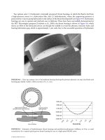
ated cavity (a SEM view of one of the sensors is provided in Figure 15.3). The vacuum cavity provided ther-
mal isolation against heat conduction to the substrate in order to maximize sensor cooling by the flow. The
resulting sensitivity was about 15 mV/Pa, and the frequency response of the sensors was 10 kHz.
Towards MEMS Autonomous Control of Free-shear Flows 15-9
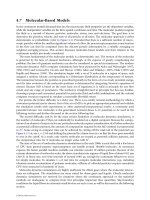
FIGURE 15.2 End (left) and plan (right) visualization of the flow around a delta wing at high angle of attack.
© 2006 by Taylor & Francis Group, LLC
Because of directional ambiguity of hot-wire measurements and the three-dimensionality of the sep-
aration line, it was not possible to identify the location of separation from the instantaneous shear-stress
values measured by the MEMS sensors. Instead, Lee et al. (1996) defined the location of the separation
line as that separating the pressure- and suction-side flows in the vicinity of the edge of the wing. The dis-
tinction between the pressure and suction sides was based on the rms level of the wall-shear signal. This
was possible because the unsteady separating flow on the suction side produced a highly fluctuating wall-
shear signature in comparison to the more steady attached flow on the pressure side.

A typical variation in the rms value of the wall-shear sensor is shown as a function of the position
around the leading edge of the wing in Figure 15.4.Note that the position around the edge is expressed in
terms of the angle from the bottom side of the edge, as demonstrated by the inset in Figure 15.4. Because
the rms is a time-integrated quantity, the detection criterion was primarily useful in identifying the average
location of separation. In a more dynamic situation where, for example, the wing is undergoing a pitching
motion, different criteria or sensor types should be used to track the instantaneous location of separation.
To map the separation position along the edge of the wing, Ho et al. (1998) utilized 64 hot-wire sensors
that were integrated during the fabrication process on a flexible shear stress skin. This 80 µm thick skin,
shown in Figure 15.5, covered a 1 ϫ 3cm
2
area and was wrapped around the curved leading edge of the delta
wing. Using the rms criterion discussed in the previous paragraph, the separation line was identified for
different flow speeds. A plot demonstrating the results is given in Figure 15.6, where the angle at which
separation occurs (see inset in Figure 15.4 for definition of the angle) is plotted as a function of the distance
from the wing apex. As seen from the figure, the separation line is curved, demonstrating the three-
dimensional nature of the separation. Additionally, the separation point seems to move closer to the pressure
side of the wing with increasing flow velocity (more details may be found in [Jiang et al., 2000]).
15.4.2 Actuation
Two different types of actuators were fabricated for use in the MEMS rolling-moment control system: (1)
magnetic flap actuators, and (2) bubble actuators. The electromagnetic driving mechanism of the former
was selected because of its ability to provide larger forces and displacements than the more common elec-
trostatic type. Passive as well as active versions of the magnetic actuator were conceived. In the passive
design, a 1 ϫ 1 mm
2
ploysilicon flap (Figure 15.7) was supported by two flexible straight beams on a sub-
strate.A 5µm thick permalloy (80% Ni and 20% Fe) was electroplated on the surface of the 1.8µm thick flap.
15-10 MEMS: Applications
FIGURE 15.3 SEM image of the UCLA/Caltech shear stress sensor.
© 2006 by Taylor & Francis Group, LLC
Towards MEMS Autonomous Control of Free-shear Flows 15-11

0
2
4
6
8
10
0 20 40 60 80 100
rms (mV)
MEMS shear
sensor
Wing edge

°
FIGURE 15.4 Distribution of surface-shear stress rms values around the edge of the delta wing.
FIGURE 15.5 UCLA/Caltech flexible shear-stress sensor array skin.
0
20
40
60
80
100
0 5 10 15 20 25 30 35
Distance from apex (cm)
30 m/s
20 m/s
10 m/s
°
FIGURE 15.6 Separation line along the edge of the delta wing for different flow velocities.
© 2006 by Taylor & Francis Group, LLC
The permalloy layer caused the flap to align itself with the magnetic field lines of a permanent magnet.

Hence, it was possible to move the flap up or downbyrotating a magnet embedded inside the edge of the
wing as seen in Figure 15.8. The actuator is described in more detail in Liu et al. (1995).
A photograph of the active flap actuator is shown in Figure 15.9. The construction of this device is gen-
erally the same as that of the passive one, except for a copper coil deposited on the silicon nitride flap. A
time varying current can be passed through the coil to modulate the flap motion around an average posi-
tion (determined by the permalloy layer electroplated on the flap and the magnetic field imposed by an
external permanent magnet). The actuator response was characterized by Tsao et al. (1994). The results
demonstrated the ability of the actuator to produce tip displacements of more than 100µm at frequen-
cies of more than 1 kHz.
To develop more robust actuators that are not only useable in wind tunnels but also in practice,
Grosjean et al. (1998) fabricated “balloon,”or bubble, actuators. The basic principle of these actuators is based
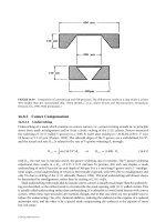
on inflating flush-mounted flexible silicon membranes using pressurized gas. As seen in Figure 15.10, the
gas can be supplied through ports that are integrated under the membrane during the microfabrication
process. When, inflated, the bubbles can extend to heights close to 1mm. Figure 15.11 demonstrates bubble
inflation with increasing pressure.
15.4.3 Flow Control
To test the ability of the actuators to produce a significant change in the roll moment on a delta wing, a 56.5°
swept-angle model was used. The model, which was 30 cm long and 1.47 cm thick, was placed inside a
91 cm
2
test section of an open return wind tunnel. For different angles of attack and flow speeds, the
moment and forces on the wing were measured using a six-component force/moment transducer.
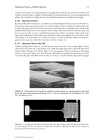
Figures 15.12a through 15.12d display measurements of the change in the rolling moment as a function
of the location of the actuator around the leading edge of the wing. Each of the four plots in Figure 15.12
15-12 MEMS: Applications
FIGURE 15.7 SEM view of passive-type flap actuators.
© 2006 by Taylor & Francis Group, LLC
represents data acquired at a different angle of attack:
α
ϭ 20°, 25°, 30°, and 35° for plots a through d respec-

tively. Also, different lines represent different Reynolds numbers.
The results shown in Figure 15.12 were obtained for the magnetic flap actuators. However, similar results
were also produced using bubble actuators [Ho et al., 1998]. In all cases, the actuators were deflected by
2 mm only on one side of the wing. The results demonstrate a significant change in the rolling moment (up
to 40% for
α
ϭ 25) for all angles of attack. The largest positive roll moment (rolling toward the actuation
side) change is observed around an actuator location of approximately 50° from the pressure side of the
wing. The location of maximum influence was found to be slightly upstream of the separation line (iden-
tified earlier using the MEMS sensor array; see Figure 15.4) as anticipated. Another important feature in
Figure 15.12 is the apparent collapse of the different lines, which suggests that the actuation impact is
affected very little, if any, by the changing Reynolds number.
In addition to producing a net positive roll moment, the miniature actuators are also capable of pro-
ducing net negative moment at the lower angles of attack as implied by the negative peak depicted in
Towards MEMS Autonomous Control of Free-shear Flows 15-13
Actuator on Actuator off
Permanent
magnet
Wing
edge
Actuator
FIGURE 15.8 Permanent magnet actuation mechanism inside delta wing.
FIGURE 15.9 SEM view of active-type flap actuator.
1.4 mm
2.0 mm
0.3 mm
8.6 mm
9.5 mm
Silicon rubber, 120 µm
Parylene C, 1.6 µm

FIGURE 15.10 Schematic of bubble actuator details.
© 2006 by Taylor & Francis Group, LLC
Figures 15.12a and 15.12b. Although, the largest negative roll value (found for an actuator location of
approximately 100° from the pressure side) is not as strong as the largest positive moment, it can be used
to augment the total roll moment control authority in a particular direction by using a two-sided actuation
scheme. That is, if actuators at the appropriate locations on both edges of the delta wing were operated
simultaneously to produce an upward motion on one side and a downward motion on the other, the two
effects would superimpose to produce a larger net rolling moment. This type of moment augmentation was
verified by Lee et al. (1996), as seen from the plot in Figure 15.13.An interesting aspect of the results shown
in Figure 15.13 is that the net rolling moment produced by the two-sided actuation is equal to the sum
of the moments produced by actuation on either side individually. This seems to suggest that the manip-
ulation of each of the vortices is independent of the other.
From a physical point of view, the production of a net rolling moment by the upward motion of the actu-
ator is caused by a resulting shift in the location of the nearby-vortex core. This was demonstrated clearly in
the flow visualization images from Ho et al. (1998). Two of these images may be seen in Figure 15.14.In
each image, a light-sheet cut was used to make the cores of the two edge vortices visible. The top image
corresponds to the flow without actuation, whereas the bottom one was captured when the right-side actu-
ators (of the bubble type in this case) were activated. A clear outward-shift of approximately one vortex
15-14 MEMS: Applications
2 k cycles
5 k cycles
11 k cycles
0 cycles
4 psi
5 psi
6 psi
7 psi
8 psi
9 psi
10 psi

800
900
1000
700
600
500
400
300
200
100
0
0 1 2 3 4 5 6 7
Pressure (psi)
Deflection (µm)
(a)
(b)
FIGURE 15.11 Bubble actuators (a) and their characteristics (b).
© 2006 by Taylor & Francis Group, LLC
diameter is observed for the right-side vortex core. Acorresponding shift in the surface-pressure signature
of the vortex presumably produces the observed net rolling moment.
The amount of vortex-core shift and resulting net moment appear to be proportional to the actuation
stroke. This can be seen from the results in Figure 15.15, where the change in rolling moment due to actua-
tion on one side is displayed for two different actuator displacements, 1 and 2mm.As observed from the data,
the peak moment produced by the 2mm actuator is about five times larger than that produced by the 1mm
actuator. It is unclear, however, if the increase in the moment is a linear or nonlinear function of the actuator
size, or stroke. In either case, the ability to adjust the amount of moment produced through the actuation
scheme is essential if proportional control of the rolling moment is desired.
Towards MEMS Autonomous Control of Free-shear Flows 15-15
–20
–10

0
10
20
30
40
0 20 40 60 80 100 120 140
2.10 × 10
5
3.15 × 10
5
4.20 × 10
5
5.25 × 10
5
Change of normalized
roll moment (%)
Re
°
(a)
–20
–10
0
10
20
30
40
0 20 40 60 80 100 120 140
Change of normalized
roll moment (%)
°

(b)
–20
–10
0
10
20
30
40
0 20 40 60 80 100 120 140
Change of normalized
roll moment (%)
°
(d)
–20
–10
0
10
20
30
40
0 20 40 60 80 100 120 140
Change of normalized
roll moment (%)
°
(c)
FIGURE 15.12 Actuation effect on delta wing rolling moment for different angles of attack: (a) 20°; (b) 25°; (c) 30°;
(d) 35°.
0
10
20

30
40
50
60
0×10
0
2×10
5
4×10
5
6×10
5
8×10
5
1×10
6
Two-sided actuation
Sum of the right- and left-sided actuation
Change of normalized
roll moment (%)
Re
FIGURE 15.13 Roll moment augmentation using two-sided actuation.
© 2006 by Taylor & Francis Group, LLC
15-16 MEMS: Applications
FIGURE 15.14 Flow visualization of the vortex structure on the suction side of the delta wing without (top) and
with (bottom) actuation.
–20
–10
0
10

20
30
40
–20
–10
0
10
20
30
40
0 20 40 60 80 100 120 140
Change of normalized
roll moment (%)
0 20 40 60 80 100 120 140
Change of normalized
roll moment (%)
°
°
FIGURE 15.15 Effect of actuation amplitude on roll moment: 1 mm (top) and 2 mm (bottom).
© 2006 by Taylor & Francis Group, LLC
Finally, Lee et al. (1996) also demonstrated that the utility of the delta wing control system is not limited
to the roll component of the moment vector. The ability to control the pitch and yaw moments as well was
demonstrated.
15.4.4 System Integration
Although sensing and actuation components of the MEMS roll-moment control system were fabricated and
demonstrated successfully by the UCLA/Caltech group, a demonstration of the full integrated system in
operation is yet to take place; that is, a demonstration of a real-time control action whereby the separation
location is detected by the hot-wire sensor array and the output is fed to the appropriate algorithms to engage
the actuators along the separation line — all done autonomously and for dynamic separation line conditions.
Such a demonstration is perhaps more challenging from a fluid mechanics perspective than from the tech-

nology, or MEMS, point of view.
So far the work conducted by the UCLA/Caltech group has shown the ability to use MEMS to fabricate
the sensors and actuators necessary to significantly modify the rolling moment on a delta wing (at least at
the scale of the test model and under controlled wind tunnel conditions). This includes the compatibility
of the fabrication processes of the sensor and actuators so that they can be integrated in arrays on the same
substrate. However, from a fluid mechanics point of view, the use of hot wires to detect the location of
dynamic three-dimensional separation is almost impossible. This is particularly true if real-time control is
to be implemented where the separation position is to be located instantaneously rather than on average.
Finally, it should be added here that the UCLA/Caltech group has recently collaborated with
AeroVironment to develop an instrumented research unmanned aerial vehicle (UAV) for testing of advanced
MEMS control concepts for maneuvering of aircraft. The vehicle, which was called GRYPHON, is shown in
the photograph in Figure 15.16.
15.5 Control of Supersonic Jet Screech
Reminiscent of several early efforts aimed at developing MEMS sensor–actuator systems for flow control, this
study involved the collaboration of fluid dynamics researchers from the Illinois Institute of Technology (IIT)
Towards MEMS Autonomous Control of Free-shear Flows 15-17
FIGURE 15.16 GRYPHON, the UCLA/Caltech MEMS flight research UAV.
© 2006 by Taylor & Francis Group, LLC
and microfabrication experts from the Center for Integrated Sensors and Circuits, Solid-State Electronics
Laboratory at the University of Michigan (UM). The selection of supersonic screech noise for the scope of
the MEMS control system was motivated by the desire to push and, therefore, identify the limits of MEMS
technology rather than by the eventual practical implementation of such a system. That is, the jet screech
environment provided harsh high-speed flow surroundings within which the devices not only had to
operate but also produce a significant disturbance of the flow.
To e xplain further, it is useful to describe the general characteristics of jet screech. When a supersonic jet
is operating at an off-designMachnumber (i.e.,the jet is under- or over-expanded), a set of shock cells forms.
These cells interact with the axi-symmetric or helical flow structures that originate from the instability of the
shear layer surrounding the jet at its exit to produce acoustic noise. The noise is primarily radiated in the
upstream direction, where it excites the jet shear layer regenerating the flow structure. Thus, a self-sustained
feedback cycle (first recognized by [Powel, 1953]) is established during screech.

The basic principle of the proposed IIT/UM screech control strategy is that of mode cancellation.
Because the existence of axi-symmetric or helical shear layer modes is a necessary link in the screech genera-
tion chain of events, their elimination or weakening is anticipated to result in a corresponding cancellation
or attenuation of screech noise. Such an elimination is to be achieved by the independent excitation of a flow
structure of the same mode shape as, but out of phase with, that existing in the shear layer using MEMS
actuators that are distributed around the nozzle lip. Since the MEMS forcing is achieved at the jet lip, where
the shear layer stability growth is likely to be linear, the natural and forced disturbances will superpose
destructively to weaken the shear layer structure. Also, the placement of the actuators in the immediate vicin-
ity of the jet lip, or point of separation of the shear layer, renders the flow susceptible to the minute distur-
bances produced by the MEMS actuators.
The spatially-fixed location of the shear layer separation point in the jet flow alleviates the need for using
sensor arrays to detect and locate the point of separation. Nevertheless,sensors are needed to provide reference
information concerning the mode shape and phase of the existing shear layer structure. In this manner, the
appropriate forcing phase of the actuators can be selected and adjusted with varying flow conditions.
15.5.1 Sensing
The IIT/UM group developed two types of sensors to provide the necessary measurements: hot wires and
microphones. The hot wires were intended for direct measurements of the disturbance velocity in the
shear layer near the nozzle lip, while the microphones were aimed at measuring the feedback acoustic
waves that generate the disturbances during screech, as explained above. A close-up view of one of the
MEMS hot wires overhanging a glass substrate is shown in Figure 15.17.Briefly, the hot wire is made from
p
ϩϩ
polysilicon with typical dimensions of 12 µm thickness, 4 µmwidth, and 100µm length. The corre-
sponding resistance is in the range of 200–800 Ω.The glass substrate under the wire provides a good
thermal-insulating base. Fabrication details are provided in Huang et al. (1996).
A sample calibration of one of the hot wires is shown in Figure 15.18 when the wire was operated at
an overheat ratio of 1.05. Three different calibrations separated by time intervals of one hour and ten days
are included in the figure. The calibration results display a change of about 2 volts of the hot-wire output
for a velocity range of up to 35 m/s. Aconventional hot wire at even larger overheats of more than 1.5
would exhibit a voltage output range of less than 1 volt. Hence, Figure 15.18 demonstrates the high sen-

sitivity of MEMS (polysilicon) hot wires. Furthermore, considering the calibration results from the three
different trials, very little change in the sensor characteristics is observed. Given the long time interval
between some of the calibrations, the MEMS sensors are generally very stable. Further characterization
of the sensors may be found in Naguib et al. (1999b).
On the other hand, the MEMS acoustic sensor, shown using a SEM view in Figure 15.19,consists of a
stress-compensated PECVD silicon nitride/oxide, 0.4 µm thick diaphragm together with four monocrys-
talline ion-implanted p
ϩϩ
silicon piezoesistors. The coefficient
π
44
for this type of piezoresistor is about
four times larger than that based on p-type polysilicon, thus leading to a higher transducer sensitivity.
The piezoresistors are arranged in a full Wheatstone-bridge configuration for detection of the diaphragm
deflection. For fabrication details, the reader is referred to Huang et al. (1998).
15-18 MEMS: Applications
© 2006 by Taylor & Francis Group, LLC
Towards MEMS Autonomous Control of Free-shear Flows 15-19
FIGURE 15.17 SEM view of the IIT/UM hot-wire sensor.
7.0
7.5
8.0
8.5
9.0
9.5
10.0
0.0 5.0 10.0 15.0 20.0 25.0 30.0 35.0
Reference
1 hr later
10 days later

HW #1
r =1.05
E
w
(V)
U (m/s)
FIGURE 15.18 Static calibration of one of the IIT/UM hot-wire sensors.
rlm
Diaphragm
Equalization
channel
FIGURE 15.19 SEM view of IIT/UM acoustic sensor.
© 2006 by Taylor & Francis Group, LLC
Figure 15.20 depicts the frequency characteristics of a 710 ϫ 710µm
2
MEMS sensor obtained by Huang
et al. (2002a). For reference, the sensitivities of acommercial silicon Kulite sensor and a 1/8Љ B&K micro-
phone are also provided in the figure. The open and closed circles represent calibration results for the
same sensor obtained two-months apart. The results demonstrate a very good agreement between the open
and closed circles. This agreement indicates that the MEMS transducers are stable and reliable. For fre-
quencies below 1kHz, the sensitivity of the MEMS sensors seems to be almost an order of magnitude larger
than the sensitivity of the commercial Kulite sensor. At higher frequencies, however, the MEMS sensitivity
is attenuated.
15.5.2 Actuation
The most common form of excitation of high-speed jets and shear layers has been via internal and external
acoustic sources (e.g. [Moore, 1977]). The popularity of acoustic forcing has been due primarily to ease
of implementation and the ability to generate the high-frequency disturbances required for effective forcing
of high-speed shear flows. However, the receptivity of the jet to acoustic excitation requires matching of
the wavenumbers of the acoustic and instability waves [Tam, 1986]. Although such a condition is achiev-
able in supersonic jets, at lowMachnumbers the instability wavelength is much smaller than the acoustic

wavelength. In this case, conversion of acoustic energy into instability waves is dependent on the efficiency
of the unsteady Kutta condition at the nozzle lip.
Historically, studies utilizing mechanical actuators have been limited to low flow speeds due to the
inability of the mechanical actuators with their large inertia to operate at frequencies higher than tens to
hundreds of herz. Therefore, the emergence of MEMS carried with it a hope to break this barrier through
the fabrication of mechanical actuators with microinertia that can oscillate at high frequency. Ultimately, this
may lead to the realization of more efficient actuators that can act directly on the flow without the need
for a Kutta-like condition. For these reasons, micromechanical actuators were selected for the screech
control problem.
Figure 15.21 shows a SEM photograph of one of the electrostatic actuators used in the jet study. The device
consists of a free-floating section that is mounted to a glass substrate underneath using elastic folded
beams. At the lower end of the floating section is a roughly 6 µm ϫ 30 µm ϫ 1300µmT-shaped actuator
head. The actuator head is made to oscillate at an amplitude up to 70µm and a resonant frequency that can
be tailored by adjusting the mass and stiffness of the actuator structure.Also, notice the porous actuator body,
which results in a reduced dynamic load on the actuator head. For more details on the construction and
manufacturing of the actuators, see Huang et al. (1996).
Two actuator designs were developed with a resonant frequency of 5 and 14 kHz. These values were
selected to match the frequency of different screech modes in the High-Speed Jet Facility (HSJF) at IIT.
The actuators were driven using a combination of 20 volt dc and a 40 volt peak-to-peak sinusoidal volt-
age at the actuator resonant frequency.
15-20 MEMS: Applications
10
–4
10
–3
10
–
2
10
–1

100 1000 10000
Kulite sensitivity
B & K sensitivity
f (Hz)
10
0
K (mV/Pa)
FIGURE 15.20 Frequency response of one of the IIT/UM acoustic sensors.
© 2006 by Taylor & Francis Group, LLC
The relative placement of one of the T-actuators with respect to the jet is illustrated in Figure 15.22. As
depicted in the figure, the rigidity of the actuator with respect to out-of-plane deflection caused by flow forces
is primarily dependent on the thickness of the device.For the device shown in Figure 15.21, the thickness
was limited to a value of less than 12 µm because of the wet etching methodology employed in the fabrica-
tion sequence. An alternate fabrication approach, which utilized deep reactive ion etching (RIE) etching,
was later utilized to fabricate thicker, more rigid actuators. Using this approach, actuators with a thickness
of 50 µmwere obtained. A SEM view of one of the thick actuators is provided in Figure 15.23.
15.5.3 Flow Control
The ability of the microactuators to disturb the shear layer surrounding the jet was tested for flow speeds of
70, 140, and 210m/s. The corresponding Mach (M
j
) and Reynolds numbers (Re; based on jet diameter, D)
were 0.2, 0.4, and 0.6 and 1,18,533, 2,37,067 and 3,55,600 respectively. The corresponding linearly most
unstable frequency of the jet shear layer was estimated to be 16, 44, and 91 kHz in order of increasing
Mach number. Because the largest effect on the flow is achieved when forcing as close as possible to the most
unstable frequency, the actuator frequency of 14 kHz was substantially lower than desired for the two
largest jet speeds.
Using hot-wire measurements on the shear layer center line, velocity spectra of the natural and forced jet
flows at the different Mach numbers were obtained. Those results are shown in Figure 15.24. The different
Towards MEMS Autonomous Control of Free-shear Flows 15-21
FIGURE 15.21 SEM view of IIT/UM electrostatic actuator.

Flow
Actuator
Flow force
Jet exit
End view Side view
FIGURE 15.22 Schematic demonstrating direction of flow forces acting on the MEMS actuator.
© 2006 by Taylor & Francis Group, LLC
15-22 MEMS: Applications
FIGURE 15.23 SEM view of a thick (50 µm) actuator.
10
–6
10
–5
10
–4
10
–3
10
–2
10
–1
10
0
0 5000 10000 15000 20000 25000 30000 35000
Natural Jet:
U
j
= 70 m/s [M
j
= 0.2]

Forced Jet:
U
j
= 70 m/s [M
j
= 0.2]
0.09
0.11
0.13
x/D
0.09
0.13
0.17
x/D
Forcing frequency
Natural Jet:
U
j
= 140 m/s [M
j
= 0.4]
0.05
0.07
0.09
x/D
0 5000 10000 15000 20000 25000 30000 35000
Forced Jet:
U
j
= 140 m/s [M

j
= 0.4]
0.05
0.07
0.09
x/D
Forcing frequency
0 5000 10000 15000 20000 25000 30000 35000
Natural Jet:
U
j
= 210 m/s [M
j
= 0.6]
0.05
0.07
0.08
x/D
0 5000 10000 15000 20000 25000 30000 35000
Forced Jet:
U
j
= 210 m/s [M
j
= 0.6]
0.05
0.07
0.10
x/D
Forcing frequency

f (Hz)
f
u′u′
(m
2
/s
2
Hz)
10
–6
10
–5
10
–4
10
–3
10
–2
10
–1
10
0
10
–6
10
–5
10
–4
10
–3

10
–2
10
–1
10
0
0 5000 10000 15000 20000 25000 30000 35000
f
u′u′
(m
2
/s
2
Hz)
10
–6
10
–5
10
–4
10
–3
10
–2
10
–1
10
0
0 5000 10000 15000 20000 25000 30000 35000
f (Hz)

f (Hz) f (Hz)
f (Hz) f (Hz)
f
u′u′
(m
2
/s
2
Hz)
f
u′u′
(m
2
/s
2
Hz)
10
–6
10
–5
10
–4
10
–3
10
–2
10
–1
10
0

10
–6
10
–5
10
–4
10
–3
10
–2
10
–1
10
0
f
u′u′
(m
2
/s
2
Hz)
f
u′u′
(m
2
/s
2
Hz)
(a)
(b)

(c)
FIGURE 15.24 Natural (left) and forced (right) spectra in the IIT high-speed jet for a Mach number of: (a) 0.2; (b) 0.4;
(c) 0.6.
© 2006 by Taylor & Francis Group, LLC
lines in each of the plots represent spectra obtained at different streamwise (x) locations. For a Mach
number of 0.2, the spectra obtained in the natural jet seem to be wide-band except for two fairly small
peaks at approximately 7 and 13 kHz. When MEMS forcing is applied, a very strong peak is observed at
the forcing frequency (Figure 15.24a,right). The magnitude of the peak seems to rise initially with down-
stream distance and then fall. In addition to the peak at the forcing frequency, a second strong peak at
28 kHz is observed at all streamwise locations. A third peak is also depicted at a frequency of 21kHz at
the second and third x locations. The existence of multiple peaks in the spectrum at frequencies that are
multiples of the forcing frequency and its subharmonic suggests that the MEMS-introduced disturbance
has a large enough amplitude to experience nonlinear effects of the flow.
The disturbance spectra for the natural jet at a Mach number of 0.4 are shown in Figure 15.24b (left).
The corresponding spectra for the forced jet are shown in Figure 15.24b (right). As seen from Figure 15.24,
the natural jet spectra possess a fairly large and broad peak at a frequency of about 13 kHz. Since the most
unstable frequency of the jet shear layer at this Mach number is expected to be around 44kHz, the 13kHz
peak does not seem to correspond to the natural mode of the shear layer or its subharmonic. When oper-
ating the MEMS actuator, a clear peak is depicted in the spectrum at the forcing frequency. The peak mag-
nitude initially magnifies to reach a magnitude of more than an order of magnitude larger than the fairly
strong peak depicted in the natural spectrum at 13kHz. The MEMS-induced peak is also significantly
sharper than the natural peak, presumably because of the more organized nature of forced modes.
Finally, the spectra obtained at a Mach number of 0.6 are displayed in Figure 15.24c. Similar to the
results for 0.4 Mach number,a broad, fairly strong peak is depicted in the natural jet spectra. The frequency
of this peak appears to be about 16 kHz at x/D ϭ 0.1, which is considerably lower than the estimated most
unstable frequency of 91kHz. The peak frequency value decreases with increasing x. This decrease in the peak
frequency with x may be symptomatic of probe feedback effects [Hussain and Zaman, 1978]. In addition
to this strong peak, when forced using the MEMS actuator, a clearly observable peak at the forcing fre-
quency is depicted in the spectrum of the forced shear layer. Unlike, the results for the forced jet at Mach
numbers of 0.2 and 0.4, the forced jet spectrum for a Mach number of 0.6 does not contain spectral peaks at

higher harmonics of the forcing frequency.
To evaluate the level of the disturbance introduced into the shear layer by the MEMS actuator, the
energy content of the spectral peak at the forcing frequency was calculated from the phase-averaged spectra
(to avoid inclusion of background turbulence energy). The forced disturbance energy (Ͻu
rms,f
Ͼ) depend-
ence on the streamwise location is shown for all three Mach numbers in Figure 42.25. The disturbance
energy is normalized by the jet velocity (U
j
), and the streamwise coordinate is normalized by the jet diam-
eter. Inspection of Figure 15.25 shows that for both Mach numbers of 0.2 and 0.4 no region of linear
growth is detectable. For these two Mach numbers, (Ͻu
rms,f
Ͼ) only increases slightly before reaching a peak
followed by a gradual decrease in value, a process that is reminiscent of nonlinear amplitude saturation.
On the other hand, the disturbance energy corresponding to a Mach number of 0.6 appears to experi-
ence linear growth over the first four streamwise positions before saturating. It appears also that only for
0.6 Mach number is the disturbance rms level appreciably lower than 1% of the jet velocity at the first
streamwise location. In the work of Drubka et al. (1989), the fundamental and subharmonic modes in an
acoustically excited incompressible axi-symmetric jet were seen to saturate when their rms value exceeded
1–2% of the jet velocity. Therefore, it seems that the IIT/UM MEMS actuator is capable of providing an
excitation to the shear layer that is sufficient not only to disturb the flow but also to produce nonlinear
forcing levels.
The magnitude of the MEMS forcing may also be appreciated further by comparison to other types of
macroscale forcing. Thus, the disturbance rms value produced by internal acoustic [Lepicovsky et al., 1985]
and glow discharge [Corke and Cavalieri, 1996] forcing is compared to the corresponding rms values pro-
duced by MEMS forcing in Figure 15.26. The results for MEMS forcing contained in the figure are those
from Huang et al. (2002b) using the high-frequency MEMS actuators as well as those from the earlier study
by Alnajjar et al. (1997) using the same type of MEMS actuators but at a forcing frequency of 5 kHz.
As seen from Figure 15.26, for most cases of MEMS forcing the MEMS-generated disturbance grows to

a level that is similar to that produced by glow discharge and acoustic forcing. For a Mach number of 0.2,
Towards MEMS Autonomous Control of Free-shear Flows 15-23
© 2006 by Taylor & Francis Group, LLC