Where.Am.I-Sensors.and.methods.for.mobile.robot.positioning.-.Borenstein(2001) Part 5 pptx

Chapter 3: Active Beacons 81
Parameter measured Performance evaluated by that parameter
Time-to-first-fix How quickly a receiver starts navigating. Not explicitly measured, but
qualitatively considered.
Static position accuracy Static accuracy and insight into overall accuracy.
Static navigation mode —
Number of satellites tracked
Taking into account DOP switching, gives insight into receiver/antenna
sensitivity.
Dynamic position plots Some accuracy information is obtained by comparing different data plots
taken while driving down the same section of road. Most of this analysis is
qualitative though because there is no ground-truth data for comparison.
Dynamic navigation mode Taking DOP switching into account gives insight into the sensitivity of the
receiver/antenna and the rate with which the receiver recovers from
obstructions.
Table 3.7: Summary of parameters measured and performance areas evaluated. (Courtesy of [Byrne, 1993].)
3.3.2.2 Test hardware
The GPS receivers tested use a serial interface for communicating position information. The
Magnavox 6400 receiver communicates using RS-422 serial communications, while the other four
receivers use the RS-232 communications standard. The RS-422 and RS-232 standards for data
transmission are compared in Table 3.8.
For the short distances involved in transmitting GPS data from the receiver to a computer, the
type of serial communications is not important. In fact, even though RS-232 communications are
inferior in some ways to RS422, RS-232 is easier to work with because it is a more common standard
(especially for PC-type computers).
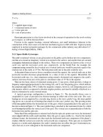
A block diagram of the overall GPS test system is shown in Figure 3.10. Figure 3.10 depicts the
system used for dynamic testing where power was supplied from a 12-Volt battery. For the static
testing, AC power was available with an extension cord. Therefore, the computer supply was
connected directly to AC, while the +12 Volts for the GPS receivers was generated using an AC-DC
power supply for the static test.
The GPS test fixture was set up in a Chevrolet van with an extended rear for additional room. The

GPS antennas were mounted on aluminum plates that where attached to the van with magnets. The
Rockwell antenna came with a magnetic mount so it was attached directly to the roof. The five
antennas were within one meter of each other near the rear of the van and mounted at the same
height so that no antenna obstructed the others.
Data
acquisition
computer
AC power
supply
DC-AC
inverter
RS-232
RS-232
RS-232
RS-422
RS-232
Interface circuit
Battery backup
Magellan OEM
Magnavox Eng.
Rockwell NavCore
Magnavox 6400
Trimble Placer
GPS receivers
12 Volt battery
byr02_01.cdr,.wpg
82 Part I Sensors for Mobile Robot Positioning
RS-232 Communications RS-422 Communications
Single-ended data transmission Differential data transmissions
Relatively slow data rates (usually < 20 kbs),

short distances up to 50 feet, most widely used.
Very high data rates (up to I0 Mbs), long distances
(up to 4000 feet at I00 Kbs), good noise immunity.
Table 3.8: Comparison of RS-232 and RS-422 serial communications. (Courtesy of [Byrne, 1993].)
Figure 3.10: Block diagram of the GPS test fixture. (Courtesy of [Byrne, 1993].)
For the dynamic testing, power was supplied from a 60 Amp-Hour lead acid battery. The battery
was used to power the AC-DC inverter as well as the five receivers. The van's electrical system was
tried at first, but noise caused the computer to lock up occasionally. Using an isolated battery solved
this problem. An AC-powered computer monitor was used for the static testing because AC power
was available. For the dynamic testing, the low power LCD display was used.
3.3.2.3 Data post processing
The GPS data was stored in raw form and post processed to extract position and navigation data.
This was done so that the raw data could be analyzed again if there were any questions with the
results. Also, storing the data as it came in from the serial ports required less computational effort
and reduced the chance of overloading the data acquisition computer. This section describes the
software used to post process the data.
Table 3.9 shows the minimum resolution (I e, the smallest change in measurement the unit can
output) of the different GPS receivers. Note, however, that the resolution of all tested receivers is
still orders of magnitude smaller than the typical position error of up to 100 meters. Therefore, this
parameter will not be an issue in the data analysis.
Chapter 3: Active Beacons 83
Receiver Data format resolution
(degrees)
Minimum resolution
(meters)
Magellan 10
-7
0.011
Magnavox GPS Engine 1.7×l0
-6

0.19
Rockwell NavCore V 5.73×l0
-10
6.36×l0
-5
Magnavox 6400 10 5.73×l0
-8 -7
6.36×l0
-2
Trimble Placer 10
-5
1.11
Table 3.9: Accuracy of receiver data formats. (Courtesy of [Byrne, 1993].)
Once the raw data was converted to files with latitude, longitude, and navigation mode in
columnar form, the data was prepared for analysis. Data manipulations included obtaining the
position error from a surveyed location, generating histograms of position error and navigation mode,
and plotting dynamic position data. The mean and variance of the position errors were also obtained.
Degrees of latitude and longitude were converted to meters using the conversion factors listed below.
Latitude Conversion Factor 11.0988×10 m/ latitude
4
Longitude Conversion Factor 9.126×10 m/ longitude
4
3.3.3 Test Results
Sections 3.3.3.1 and 3.3.3.2 discuss the test results for the static and dynamic tests, respectively,
and a summary of these results is given in Section 3.3.3.3. The results of the static and dynamic tests
provide different information about the overall performance of the GPS receivers. The static test
compares the accuracy of the different receivers as they navigate at a surveyed location. The static
test also provides some information about the receiver/antenna sensitivity by comparing navigation
modes (3D-mode, 2D-mode, or not navigating) of the different receivers over the same time period.
Differences in navigation mode may be caused by several factors. One is that the receiver/antenna

operating in a plane on ground level may not be able to track a satellite close to the horizon. This
reflects receiver/antenna sensitivity. Another reason is that different receivers have different DOP
limits that cause them to switch to two dimensional navigation when four satellites are in view but
the DOP becomes too high. This merely reflects the designer's preference in setting DOP switching
masks that are somewhat arbitrary.
Dynamic testing was used to compare relative receiver/antenna sensitivity and to determine the
amount of time during which navigation was not possible because of obstructions. By driving over
different types of terrain, ranging from normal city driving to deep canyons, the relative sensitivity
of the different receivers was observed. The navigation mode (3D-mode, 2D-mode, or not
navigating) was used to compare the relative performance of the receivers. In addition, plots of the
data taken give some insight into the accuracy by qualitatively observing the scatter of the data.
84 Part I Sensors for Mobile Robot Positioning
Surveyed Latitude Surveyed Longitude
35 02 27.71607 (deg min sec) 106 31 16.14169 (deg min sec)
35.0410322 (deg) 106.5211505 (deg)
Table 3.10: Location of the surveyed point at the Sandia Robotic Vehicle
Range. (Courtesy of [Byrne, 1993].)
Receiver Mean position error Position error standard
deviation
(meters) (feet) (meters) (feet)
Magellan 33.48 110 23.17 76
Magnavox GPS Engine 22.00 72 16.06 53
Rockwell NavCore V 30.09 99 20.27 67
Magnavox 6400 28.01 92 19.76 65
Trimble Placer 29.97 98 23.58 77
Table 3.11: Summary of the static position error mean and variance for different receivers.
(Courtesy of [Byrne, 1993].)
3.3.3.1 Static test results
Static testing was conducted at a surveyed location at Sandia National Laboratories' Robotic Vehicle
Range (RVR). The position of the surveyed location is described in Table 3.10.

The data for the results presented here was gathered on October 7 and 8, 1992, from 2:21 p.m.
to 2:04 p.m. Although this is the only static data analyzed in this report, a significant amount of
additional data was gathered when all of the receivers were not functioning simultaneously. This
previously gathered data supported the trends found in the October 7 and 8 test.The plots of the
static position error for each receiver are shown in Figure 3.11. A summary of the mean and standard
deviation ( ) of the position error for the different receivers appears in Table 3.11.
It is evident from Table 3.11 that the Magnavox GPS Engine was noticeably more accurate when
comparing static position error. The Magellan, Rockwell, Magnavox 6400, and Trimble Placer all
exhibit comparable, but larger, average position errors. This trend was also observed when SA was
turned off. However, a functioning Rockwell receiver was not available for this test so the data will
not be presented. It is interesting to note that the Magnavox 6400 unit compares well with the newer
receivers when looking at static accuracy. This is expected: since the receiver only has two channels,
it will take longer to reacquire satellites after blockages; one can also expect greater difficulties with
dynamic situations. However, in a static test, the weaknesses of a sequencing receiver are less
noticeable.
Chapter 3: Active Beacons 85
a. Magellan b. Magnavox GPS Engine.
c. Rockwell NavCore V. d. Magnavox 6400.
e. Trimble Placer.
Figure 3.11: Static position error plots for all five
GPS receivers. (Courtesy of Byrne [1993]).
10
20
30
40
50
60
70
80
90

100
0
200
400
600
800
1000
Position
error bins (in meters)
Number of
samples
86 Part I Sensors for Mobile Robot Positioning
Figure 3.12:
Histogramic error distributions for the data taken during the static test, for all five tested GPS
receivers. (Adapted from [Byrne, 1993].)
The histogramic error distributions for the data taken during the static test are shown in
Figure 3.12. One can see from Fig. 3.12 that the Magnavox GPS Engine has the most data points
within 20 meters of the surveyed position. This corresponds with the smallest mean position error
exhibited by the Magnavox receiver. The error distributions for the other four receivers are fairly
similar. The Magnavox 6400 unit has slightly more data points in the 10 to 20 meter error bin, but
otherwise there are no unique features. The Magnavox GPS Engine is the only receiver of the five
tested that had a noticeably superior static position error distribution. Navigation mode data for the
different receivers is summarized in Figure 3.13 for the static test.
In order to analyze the data in Figure 3.13, one needs to take into account the DOP criterion for
the different receivers. As mentioned previously, some receivers switch from 3D-mode navigation
to 2D-mode navigation if four satellites are visible but the DOP is above a predetermined threshold.
The DOP switching criterion for the different receivers are outlined in Table 3.12. As seen in
Table 3.12, the different receivers use different DOP criteria. However, by taking advantage of
Equations (3.1) and (3.2), the different DOP criteria can be compared.
% No Navigation % 2-D Navi gation % 3-D Navigation

0.0 0.0 0.0
1.6
0.0
17.8
2.4
2.7
2.2
6.7
82.2
97.7
97.3
96.2
93.3
Magellan Magnavox Engine Rockwell NavCore Magnavox 6400 Trimble Placer
0.0
10.0
20.0
30.0
40.0
50.0
60.0
70.0
80.0
90.0
100.0
Chapter 3: Active Beacons 87
Receiver 2-D/3-D DOP criterion PDOP equivalent
Magellan If 4 satellites visible and VDOP >7, will
switch to 2-D navigation.
Enters 3-D navigation when VDOP<5.

PDOP >
(HDOP + 7 )
22½
Magnavox GPS
Engine
If 4 satellites visible and VDOP>10,
switches to 2-D navigation.
If HDOP>10, suspends 2-D navigation
PDOP < (HDOP + 5 )
22½
PDOP > (HDOP + 10 )
22½
Rockwell NavCore V If 4 satellites visible and GDOP>13,
switches to 2-D navigation.
PDOP > (13 - TDOP )
22½
Magnavox 6400 Data Not Available in MX 5400 manual
provided
Trimble Placer If 4 satellites visible and PDOP>8, switches to 2-D
navigation. If PDOP>12, receiver stops navigating.
PDOP >
8
Table 3.12:
Summary of DOP - navigation mode switching criteria. (Courtesy of [Byrne, 1993].)
Figure 3.13:
Navigation mode data for the static test. (Adapted from [Byrne, 1993].)
Table 3.12 relates all of the different DOP criteria to the PDOP. Based on the information in
Table 3.12, several comments can be made about the relative stringency of the various DOP
criterions. First, the Magnavox GPS Engine VDOP criterion is much less stringent than the Magellan
VDOP criterion (these two can be compared directly). The Magellan unit also incorporates

hysteresis, which makes the criterion even more stringent. Comparing the Rockwell to the Trimble
Placer, the Rockwell criterion is much less stringent. A TDOP of 10.2 would be required to make
the two criteria equivalent. The Rockwell and Magnavox GPS Engine have the least stringent DOP
requirements.
Taking into account the DOP criterions of the different receivers, the significant amount of two-
dimensional navigation exhibited by the Magellan receiver might be attributed to a more stringent
DOP criterion. However, this did not improve the horizontal (latitude-longitude) position error. The
Magnavox GPS Engine still exhibited the most accurate static position performance. The same can
88 Part I Sensors for Mobile Robot Positioning
be said for the Trimble Placer unit. Although is has a stricter DOP requirement than the Magnavox
Engine, its position location accuracy was not superior. The static navigation mode results don't
conclusively show that any receiver has superior sensitivity. However, the static position error results
do show that the Magnavox GPS Engine is clearly more accurate than the other receivers tested. The
superior accuracy of the Magnavox receiver in the static tests might be attributed to more filtering
in the receiver. It should also be noted that the Magnavox 6400 unit was the only receiver that did
not navigate for some time period during the static test.
3.3.3.2 Dynamic test results
The dynamic test data was obtained by driving the instrumented van over different types of
terrain. The various routes were chosen so that the GPS receivers would be subjected to a wide
variety of obstructions. These include buildings, underpasses, signs, and foliage for the city driving.
Rock cliffs and foliage were typical for the mountain and canyon driving. Large trucks, underpasses,
highway signs, buildings, foliage, as well as small canyons were found on the interstate and rural
highway driving routes.
The results of the dynamic testing are presented in Figures 3.14 through 3.18. The dynamic test
results as well as a discussion of the results appear on the following pages.
Several noticeable differences exist between Figure 3.13 (static navigation mode) and Figure 3.14.
The Magnavox 6400 unit is not navigating a significant portion of the time. This is because
sequencing receivers do not perform as well in dynamic environments with periodic obstructions.
The Magellan GPS receiver also navigated in 2D-mode a larger percentage of the time compared
with the other receivers. The Rockwell unit was able to navigate in 3D-mode the largest percentage

of the time. Although this is also a result of the Rockwell DOP setting discussed in the previous
section, it does seem to indicate that the Rockwell receiver might have slightly better sensitivity
(Rockwell claims this is one of the receiver's selling points). The Magnavox GPS Engine also did not
navigate a small percentage of the time. This can be attributed to the small period of time when the
receiver was obstructed and the other receivers (which also were obstructed) might not have been
outputting data (caused by asynchronous sampling).
The Mountain Driving Test actually yielded less obstructions than the City Driving Test. This
might be a result of better satellite geometries during the test period. However, the Magnavox 6400
unit once again did not navigate for a significant portion of the time. The Magellan receiver
navigated in 2D-mode a significant portion of the time, but this can be attributed to some degree to
the stricter DOP limits. The performance of the Rockwell NavCore V, Trimble Placer, and
Magnavox GPS Engine are comparable.
% No Navigation % 2-D Navigation % 3-D Navigation
0.0
3.4
0.0
10.3
0.0
25.8
5.3
1.1
0.2
5.2
74.2
91.2
98
.
9
89.4
94.8

Magellan Magnavox Engine Rockwell Nav V Magnavox 6400 Trimble Placer
0.0
10.0
20.0
30.0
40.0
50.0
60.0
70.0
80.0
90.0
100.0
% No Navigation % 2-D Navigation % 3-D Navigation
0.0 0.0 0.0
4.6
0.0
12.3
1.0
0.0 0.0
1.3
87.7
99
.
0
100
.
0
95.5
98.7
Magellan Magnavox Engine Rockwell Nav V Magnavox 6400 Trimble Placer

0.0
10.0
20.0
30.0
40.0
50.0
60.0
70.0
80.0
90.0
100.0
% No Navigation % 2-D Navigation % 3-D Navigation
0.0
1.1 1.2
30.2
0.0
15.7
4.4
0.0 0.0 0.0
84.3
94.6
98
.
8
69.8
100
.
0
Magellan Magnavox Engine Rockwell Nav V Magnavox 6400 Trimble Placer
0.0

10.0
20.0
30.0
40.0
50.0
60.0
70.0
80.0
90.0
100.0
Chapter 3: Active Beacons 89
Figure 3.14:
Summary of City Driving Results. (Adapted from [Byrne, 1993]).
Figure 3.15:
Summary of mountain driving results. (Adapted from [Byrne, 1993]).
Figure 3.16:
Summary of Canyon Driving Results. (Adapted from [Byrne, 1993]).
% No Navigation % 2-D Navigation % 3-D Navigation
0.0
0.4 0.2
20.1
0.0
32.8
0.4 0.2
0.0
4.2
67.2
99
.
3

99
.
6
79.9
95.8
Magellan Magnavox Engine Rockwell Nav V Magnavox 6400 Trimble Placer
0.0
10.0
20.0
30.0
40.0
50.0
60.0
70.0
80.0
90.0
100.0
% No Navigation % 2-D Navigation % 3-D Navigation
0.0 0.3
1.6
10.4
0.0
7.4
1.3
0.5
1.8
3.9
92.7
98.5
97.8

87.8
96.1
Magellan Magnavox Engine Rockwell Nav V Magnavox 6400 Trimble Placer
0.0
10.0
20.0
30.0
40.0
50.0
60.0
70.0
80.0
90.0
100.0
90 Part I Sensors for Mobile Robot Positioning
Figure 3.17:
Summary of Interstate Highway Results. (Adapted from [Byrne, 1993]).
Figure 3.18
. Summary of Rural Highway Results. (Adapted from [Byrne, 1993]).
The Canyon Driving Test exposed the GPS receivers to the most obstructions. The steep canyon
walls and abundant foliage stopped the current receiver from navigating over 30 percent of the time.
The Magnavox GPS Engine and Rockwell receiver were also not navigating a small percentage of
the time. This particular test clearly shows the superiority of the newer receivers over the older
sequencing receiver. Because the newer receivers are able to track extra satellites and recover more
quickly from obstructions, they are better suited for operation in dynamic environments with
periodic obstructions. The Trimble Placer and Rockwell receiver performed the best in this particular
test, followed closely by the Magnavox GPS Engine.
During the Interstate Highway Driving tests, the Magnavox 6400 unit did not navigate over
20 percent of the time. This is consistent with the sometimes poor performance exhibited by the
current navigation system. The other newer receivers did quite well, with the Trimble Placer,

Magnavox GPS Engine, and Rockwell NavCore V exhibiting similar performance. Once again, the
Chapter 3: Active Beacons 91
Magellan unit navigated in 2D-mode a significant portion of the time. This can probably be attributed
to the stricter DOP limits.
During the Rural Highway Driving test the Magnavox 6400 unit once again did not navigate a
significant portion of the time. All of the newer receivers had similar performance results. The
Magellan receiver navigated in 2D-mode considerably less in this test compared to the other dynamic
tests.
3.3.3.3 Summary of test results
Both static and dynamic tests were used to compare the performance of the five different GPS
receivers. The static test results showed that the Magnavox GPS Engine was the most accurate (for
static situations). The other four receivers were slightly less accurate and exhibited similar static
position error performance. The static navigation mode results did not differentiate the sensitivity
of the various receivers significantly. The Magellan unit navigated in 2D-mode much more
frequently than the other receivers, but some of this can be attributed to stricter DOP limits.
However, the stricter DOP limits of the Magellan receiver and Trimble Placer did not yield better
static position accuracies. All four of the newer GPS receivers obtained a first fix under one minute,
which verifies the time to first-fix specifications stated by the manufacturers.
The dynamic tests were used to differentiate receiver sensitivity and the ability to recover quickly
from periodic obstructions. As expected, the Magnavox 6400 unit did not perform very well in the
dynamic testing. The Magnavox 6400 was unable to navigate for some period of each dynamic test.
This was most noticeable in the Canyon route, where the receiver did not navigate over 30 percent
of the time. The newer receivers performed much better in the dynamic testing, navigating almost
all of the time. The Magnavox GPS Engine, Rockwell NavCore V, and Trimble Placer exhibited
comparable receiver/antenna sensitivity during the dynamic testing based on the navigation mode
data. The Magellan unit navigated in 2D-mode significantly more than the other receivers in the
dynamic tests. Most of this can probably be attributed to a more stringent DOP requirement. It
should also be noted that the Magellan receiver was the only receiver to navigate in 2D-mode or 3D-
mode 100 percent of the time in all of the dynamic tests.
Overall, the four newer receivers performed significantly better than the Magnavox 6400 unit in

the dynamic tests. In the static test, all of the receivers performed satisfactorily, but the Magnavox
GPS Engine exhibited the most accurate position estimation. Recommendations on choosing a GPS
receiver are outlined in the next section.
3.3.4 Recommendations
In order to discuss some of the integration issues involved with GPS receivers, a list of the
problems encountered with the receivers tested is outlined in Section 3.3.4.1. The problems
encountered with the Magnavox 6400 unit (there were several) are not listed because the Magnavox
6400 unit is not comparable to the newer receivers in performance.
Based on the problems experienced testing the GPS receivers as well as the requirements of the
current application, a list of critical issues is outlined in Section 3.3.4.2.
One critical integration issue not mentioned in Section 3.3.4.2 is price. Almost any level of
performance can be purchased, but at a significantly increased cost. This issue will be addressed
further in the next section. Overall, the Magellan OEM Module, the Magnavox GPS Engine,
Rockwell NavCore V, and Trimble Placer are good receivers. The Magnavox GPS Engine exhibited
superior static position accuracy. During dynamic testing, all of the receivers were able to navigate
92 Part I Sensors for Mobile Robot Positioning
a large percentage of the time, even in hilly wooded terrain. Based on the experimental results, other
integration issues such as price, software flexibility, technical support, size, power, and differential
capability are probably the most important factors to consider when choosing a GPS receiver.
3.3.4.1 Summary of problems encountered with the tested GPS receivers
Magellan OEM Module
No problems, unit functioned correctly out of the box. However, the current drain on the battery
for the battery backed RAM seemed high. A 1-AmpHour 3.6-Volt Lithium battery only lasted a
few months.
The binary position packet was used because of the increased position resolution. Sometimes the
receiver outputs a garbage binary packet (about I percent of the time).
Magnavox GPS Engine
The first unit received was a pre-production unit. It had a difficult time tracking satellites. On one
occasion it took over 24 hours to obtain a first fix. This receiver was returned to Magnavox.
Magnavox claimed that upgrading the software fixed the problem. However, the EEPROM failed

when trying to load the oscillator parameters. A new production board was shipped and it
functioned flawlessly out of the box.
The RF connector for the Magnavox GPS Engine was also difficult to obtain. The suppliers
recommended in the back of the GPS Engine Integration Guide have large minimum orders. A
sample connector was finally requested. It never arrived and a second sample had to be
requested.
Rockwell NavCore V
The first Rockwell receiver functioned for a while, and then began outputting garbage at 600
baud (9600 baud is the only selectable baud rate). Rockwell claims that a Gallium Arsenide IC
that counts down a clock signal was failing because of contamination from the plastic package
of the IC (suppliers fault). This Rockwell unit was returned for repair under warranty.
The second Rockwell unit tested output data but did not navigate. Power was applied to the unit
with reverse polarity (Sandia's fault) and an internal rectifier bridge allowed the unit to function,
but not properly. Applying power in the correct manner (positive on the outside contact) fixed
the problem.
Trimble Placer
No problems, unit functioned correctly out of the box.
3.3.4.2 Summary of critical integration issues
Flexible software interface Having the flexibility to control the data output by the receiver is
important. This includes serial data format (TTL, RS-232, RS-422). baud rates, and packet data rates.
It is desirable to have the receiver output position data at fixed data rate, that is user selectable. It
is also desirable to be able to request other data packets when needed. All of the receivers with the
exception of the Rockwell unit were fairly flexible. The Rockwell unit on the other hand outputs
position data at a fixed 1-Hz rate and fixed baud rate of 9600 baud.
The format of the data packets is also important. ASCII formats are easier to work with because
the raw data can be stored and then analyzed visually. The Rockwell unit uses an IEEE floating point
Chapter 3: Active Beacons 93
format. Although Binary data formats and the Rockwell format might be more efficient, it is much
easier to troubleshoot a problem when the data docs not have to be post processed just to take a
quick look.

Differential capability The capability to receive differential corrections is important if increased
accuracy is desired. Although a near-term fielded system might not use differential corrections, the
availability of subscriber networks that broadcast differential corrections in the future will probably
make this a likely upgrade.
Time to first fix A fast time-to-first-fix is important. However, all newer receivers usually advertise
a first fix in under one minute when the receiver knows its approximate position. The difference
between a 30-second first fix and a one-minute first fix is probably not that important. This
parameter also affects how quickly the receiver can reacquire satellites after blockages.
Memory back up Different manufacturers use different approaches for providing power to back
up the static memory (which stores the last location, almanac, ephemeris, and receiver parameters)
when the receiver is powered down. These include an internal lithium battery, an external voltage
supplied by the integrator, and a large capacitor. The large capacitor has the advantage of never
needing replacement. This approach is taken on the Rockwell NavCore V. However, the capacitor
charge can only last for several weeks. An internal lithium battery can last for several years, but will
eventually need replacement. An external voltage supplied by the integrator can come from a
number of sources, but must be taken into account when doing the system design.
Size, Power, and packaging Low power consumption and small size are advantageous for vehicular
applications. Some manufacturers also offer the antenna and receiver integrated into a single
package. This has some advantages, but limits antenna choices.
Active/passive antenna Active antennas with built-in amplifiers allow longer cable runs to the
receiver. Passive antennas require no power but can not be used with longer cabling because of
losses.
Cable length and number of connectors The losses in the cabling and connectors must be taken
into account when designing the cabling and choosing the appropriate antenna.
Receiver/antenna sensitivity Increased receiver/antenna sensitivity will reduce the affects of
foliage and other obstructions. The sensitivity is affected by the receiver, the cabling, as well as the
antenna used.
Position accuracy Both static and dynamic position accuracy are important. However, the effects
of SA reduce the accuracy of all receivers significantly. Differential accuracy will become an
important parameter in the future.

Technical Support Good technical support, including quick turn around times for repairs, is very
important. Quick turn around for failed units can also be accomplished by keeping spares in stock.
94 Part I Sensors for Mobile Robot Positioning
This Page intentionally left blank.
C
HAPTER
4
S
ENSORS FOR
M
AP
-B
ASED
P
OSITIONING
Most sensors used for the purpose of map building involve some kind of distance measurement.
There are three basically different approaches to measuring range:
Sensors based on measuring the time of flight (TOF) of a pulse of emitted energy traveling to a
reflecting object, then echoing back to a receiver.
The phase-shift measurement (or phase-detection) ranging technique involves continuous wave
transmission as opposed to the short pulsed outputs used in TOF systems.
Sensors based on frequency-modulated (FM) radar. This technique is somewhat related to the
(amplitude-modulated) phase-shift measurement technique.
4.1 Time-of-Flight Range Sensors
Many of today's range sensors use the time-of-flight (TOF) method. The measured pulses typically
come from an ultrasonic, RF, or optical energy source. Therefore, the relevant parameters involved
in range calculation are the speed of sound in air (roughly 0.3 m/ms — 1 ft/ms), and the speed of
light (0.3 m/ns — 1 ft/ns). Using elementary physics, distance is determined by multiplying the
velocity of the energy wave by the time required to travel the round-trip distance:
d = v t (4.1)

where
d = round-trip distance
v = speed of propagation
t = elapsed time.
The measured time is representative of traveling twice the separation distance (i.e., out and back)
and must therefore be reduced by half to result in actual range to the target.
The advantages of TOF systems arise from the direct nature of their straight-line active sensing.
The returned signal follows essentially the same path back to a receiver located coaxially with or in
close proximity to the transmitter. In fact, it is possible in some cases for the transmitting and
receiving transducers to be the same device. The absolute range to an observed point is directly
available as output with no complicated analysis required, and the technique is not based on any
assumptions concerning the planar properties or orientation of the target surface. The missing parts
problem seen in triangulation does not arise because minimal or no offset distance between
transducers is needed. Furthermore, TOF sensors maintain range accuracy in a linear fashion as long
as reliable echo detection is sustained, while triangulation schemes suffer diminishing accuracy as
distance to the target increases.
Potential error sources for TOF systems include the following:
Variations in the speed of propagation, particularly in the case of acoustical systems.
Uncertainties in determining the exact time of arrival of the reflected pulse.
96 Part I Sensors for Mobile Robot Positioning
Inaccuracies in the timing circuitry used to measure the round-trip time of flight.
Interaction of the incident wave with the target surface.
Each of these areas will be briefly addressed below, and discussed later in more detail.
a. Propagation Speed For mobile robotics applications, changes in the propagation speed of
electromagnetic energy are for the most part inconsequential and can basically be ignored, with the
exception of satellite-based position-location systems as presented in Chapter 3. This is not the case,
however, for acoustically based systems, where the speed of sound is markedly influenced by
temperature changes, and to a lesser extent by humidity. (The speed of sound is actually proportional
to the square root of temperature in degrees Rankine.) An ambient temperature shift of just 30 F
o

can cause a 0.3 meter (1 ft) error at a measured distance of 10 meters (35 ft) [Everett, 1985].
b. Detection Uncertainties So-called time-walk errors are caused by the wide dynamic range
in returned signal strength due to varying reflectivities of target surfaces. These differences in
returned signal intensity influence the rise time of the detected pulse, and in the case of fixed-
threshold detection will cause the more reflective targets to appear closer. For this reason, constant
fraction timing discriminators are typically employed to establish the detector threshold at some
specified fraction of the peak value of the received pulse [Vuylsteke et al., 1990].
c. Timing Considerations Due to the relatively slow speed of sound in air, compared to light,
acoustically based systems face milder timing demands than their light-based counterparts and as a
result are less expensive. Conversely, the propagation speed of electromagnetic energy can place
severe requirements on associated control and measurement circuitry in optical or RF implementa-
tions. As a result, TOF sensors based on the speed of light require sub-nanosecond timing circuitry
to measure distances with a resolution of about a foot [Koenigsburg, 1982]. More specifically, a
desired resolution of 1 millimeter requires a timing accuracy of 3 picoseconds (3×10 s) [Vuylsteke
-12
et al., 1990]. This capability is somewhat expensive to realize and may not be cost effective for
certain applications, particularly at close range where high accuracies are required.
d. Surface Interaction When light, sound, or radio waves strike an object, any detected echo
represents only a small portion of the original signal. The remaining energy reflects in scattered
directions and can be absorbed by or pass through the target, depending on surface characteristics
and the angle of incidence of the beam. Instances where no return signal is received at all can occur
because of specular reflection at the object's surface, especially in the ultrasonic region of the energy
spectrum. If the transmission source approach angle meets or exceeds a certain critical value, the
reflected energy will be deflected outside of the sensing envelope of the receiver. In cluttered
environments soundwaves can reflect from (multiple) objects and can then be received by other
sensors. This phenomenon is known as crosstalk (see Figure 4.1). To compensate, repeated
measurements are often averaged to bring the signal-to-noise ratio within acceptable levels, but at
the expense of additional time required to determine a single range value. Borenstein and Koren
[1995] proposed a method that allows individual sensors to detect and reject crosstalk.
Mobile

robot
Mobile
robot
X
y
y
y
y
y
y
X
y
y
y
y
y
y
a.
b.
Direction
of motion
\eeruf\crostalk.ds4, crostalk.wmf
Chapter 4: Sensors for Map-Based Positioning 97
Figure 4.1:
Crosstalk is a phenomenon in which one sonar picks
up the echo from another. One can distinguish between a. direct
crosstalk and b. indirect crosstalk.
Using this method much faster firing
rates — under 100 ms for a complete
scan with 12 sonars — are feasible.

4.1.1 Ultrasonic TOF Systems
Ultrasonic TOF ranging is today the
most common technique employed on
indoor mobile robotics systems, pri-
marily due to the ready availability of
low-cost systems and their ease of
interface. Over the past decade, much
research has been conducted investi-
gating applicability in such areas as
world modeling and collision avoid-
ance, position estimation, and motion
detection. Several researchers have
more recently begun to assess the
effectiveness of ultrasonic sensors in
exterior settings [Pletta et al., 1992;
Langer and Thorpe, 1992; Pin and Watanabe, 1993; Hammond, 1994]. In the automotive industry,
BMW now incorporates four piezoceramic transducers (sealed in a membrane for environmental
protection) on both front and rear bumpers in its Park Distance Control system [Siuru, 1994]. A
detailed discussion of ultrasonic sensors and their characteristics with regard to indoor mobile robot
applications is given in [Jörg, 1994].
Two of the most popular commercially available ultrasonic ranging systems will be reviewed in
the following sections.
4.1.1.1 Massa Products Ultrasonic Ranging Module Subsystems
Massa Products Corporation, Hingham, MA, offers a full line of ultrasonic ranging subsystems with
maximum detection ranges from 0.6 to 9.1 meters (2 to 30 ft) [MASSA]. The E-201B series sonar
operates in the bistatic mode with separate transmit and receive transducers, either side by side for
echo ranging or as an opposed pair for unambiguous distance measurement between two uniquely
defined points. This latter configuration is sometimes used in ultrasonic position location systems and
provides twice the effective operating range with respect to that advertised for conventional echo
ranging. The E-220B series (see Figure 4.2) is designed for monostatic (single transducer) operation

but is otherwise functionally identical to the E-201B. Either version can be externally triggered on
command, or internally triggered by a free-running oscillator at a repetition rate determined by an
external resistor (see Figure 4.3).
Selected specifications for the four operating frequencies available in the E-220B series are listed
in Table 4.1 below. A removable focusing horn is provided for the 26- and 40-kHz models that
decreases the effective beamwidth (when installed) from 35 to 15 degrees. The horn must be in place
to achieve the maximum listed range.
Analog
Latch
GND
+V
Filter
cc
Trig in
Trig out
PRR
Internal
oscillator
Transmit
driver
timing
Digital
G
S
D
Threshold
Receiver
AC
AMP
V

Pulse repetition rate period
Digital
Trigger
Analog
Ring down
2nd echo1st echo
98 Part I Sensors for Mobile Robot Positioning
Figure 4.2: The single-transducer Massa
E-220B
-
series
ultrasonic ranging module
can be internally or externally triggered, and offers both analog and digital outputs.
(Courtesy of Massa Products Corp.)
Figure 4.3: Timing diagram for the
E-220B

series
ranging module showing
analog and digital output signals in relationship to the trigger input. (Courtesy
of Massa Products Corp.)
Parameter E-220B/215 E-220B/150 E-220B/40 E-220B/26 Units
Range 10 - 61
4 - 24
20 - 152
8 - 60
61 - 610
24 - 240
61 - 914
24 - 360

cm
in
Beamwidth 10 10 35 (15) 35 (15)
Frequency 215 150 40 26 kHz
Max rep rate 150 100 25 20 Hz
Resolution 0.076
0.03
0.1
0.04
0.76
0.3
1
0.4
cm
in
Power 8 - 15 8 - 15 8 - 15 8 - 15 VDC
Weight 4 - 8 4 - 8 4 - 8 4 - 8 oz
Table 4.1: Specifications for the monostatic E-220B Ultrasonic Ranging Module Subsystems. The E-201
series is a bistatic configuration with very similar specifications. (Courtesy of Massa Products Corp.)
Chapter 4: Sensors for Map-Based Positioning 99
Figure 4.4: The Polaroid OEM kit included the transducer and a small
electronics interface board.
Figure 4.5: The Polaroid instrument grade electrostatic transducer
consists of a gold-plated plastic foil stretched across a machined
backplate. (Reproduced with permission from Polaroid [1991].)
4.1.1.2 Polaroid Ultrasonic Ranging Modules
The Polaroid ranging module is
an active TOF device developed
for automatic camera focusing,
which determines the range to

target by measuring elapsed
time between the transmission
of an ultrasonic waveform and
the detected echo [Biber et al.,
1987, POLAROID]. This sys-
tem is the most widely found in
mobile robotics literature
[Koenigsburg, 1982; Moravec
and Elfes, 1985; Everett, 1985;
Kim, 1986; Moravec, 1988;
Elfes, 1989; Arkin, 1989;
Borenstein and Koren, 1990;
1991a; 1991b; 1995; Borenstein
et al., 1995], and is representa-
tive of the general characteris-
tics of such ranging devices. The most basic configuration consists of two fundamental components:
1) the ultrasonic transducer, and 2) the ranging module electronics. Polaroid offers OEM kits with
two transducers and two ranging module circuit boards for less than $100 (see Figure 4.4).
A choice of transducer types is now available. In the original instrument-grade electrostatic
version, a very thin metal diaphragm mounted on a machined backplate formed a capacitive
transducer as illustrated in Figure 4.5 [POLAROID, 1991]. The system operates in the monostatic
transceiver mode so that only a single transducer is necessary to acquire range data. A smaller
diameter electrostatic trans-
ducer (7000-series) has also
been made available, developed
for the Polaroid Spectra camera
[POLAROID, 1987]. A more
rugged piezoelectric (9000-se-
ries) environmental transducer
for applications in severe envi-

ronmental conditions including
vibration is able to meet or ex-
ceed the SAE J1455 January
1988 specification for heavy-
duty trucks. Table 4.2 lists the
technical specifications for the
different Polaroid transducers.
The original Polaroid ranging
module functioned by transmit-
ting a chirp of four discrete fre-
100 Part I Sensors for Mobile Robot Positioning
Parameter Original SN28827 6500 Units
Maximum range 10.5
35
10.5
35
10.5
35
m
ft
Minimum range* 25
10.5
20
6
20
6
cm
in
Number of pulses 56 16 16
Blanking time 1.6 2.38 2.38 ms

Resolution 1 2 1 %
Gain steps 16 12 12
Multiple echo no yes yes
Programmable frequency no no yes
Power 4.7 - 6.8 4.7 - 6.8 4.7 - 6.8 V
200 100 100 mA
* with custom electronics (see [Borenstein et al., 1995].)
Table 4.2: Specifications for the various Polaroid ultrasonic ranging modules. (Courtesy of
Polaroid.)
quencies at about of 50 kHz. The SN28827 module was later developed with reduced parts count,
lower power consumption, and simplified computer interface requirements. This second-generation
board transmits only a single frequency at 49.1 kHz. A third-generation board (6500 series)
introduced in 1990 provided yet a further reduction in interface circuitry, with the ability to detect
and report multiple echoes [Polaroid, 1990]. An Ultrasonic Ranging Developer’s Kit based on the
Intel 80C196 microprocessor is now available for use with the 6500 series ranging module that
allows software control of transmit frequency, pulse width, blanking time, amplifier gain, and
maximum range [Polaroid, 1993].
The range of the Polaroid system runs from about 41 centimeters to 10.5 meters (1.33 ft to 35 ft).
However, using custom circuitry suggested in [POLAROID, 1991] the minimum range can be
reduced reliably to about 20 centimeters (8 in) [Borenstein et al., 1995]. The beam dispersion angle
is approximately 30 degrees. A typical operating cycle is as follows.
1. The control circuitry fires the transducer and waits for indication that transmission has begun.
2. The receiver is blanked for a short period of time to prevent false detection due to ringing from
residual transmit signals in the transducer.
3. The received signals are amplified with increased gain over time to compensate for the decrease
in sound intensity with distance.
4. Returning echoes that exceed a fixed threshold value are recorded and the associated distances
calculated from elapsed time.
Figure 4.6 [Polaroid, 1990] illustrates the operation of the sensor in a timing diagram. In the
single-echo mode of operation for the 6500-series module, the blank (BLNK) and blank-inhibit

(BINH) lines are held low as the initiate (INIT) line goes high to trigger the outgoing pulse train. The
internal blanking (BLANKING) signal automatically goes high for 2.38 milliseconds to prevent
transducer ringing from being misinterpreted as a returned echo. Once a valid return is received, the
echo (ECHO) output will latch high until reset by a high-to-low transition on INIT.