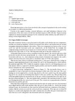
Where.Am.I-Sensors.and.methods.for.mobile.robot.positioning.-.Borenstein(2001) Part 7 doc

Chapter 4: Sensors for Map-Based Positioning 121
transmitted and received beams. More detailed specifications are listed in Table 4.13.
The 3-D Imaging Scanner is now in an advanced prototype stage and the developer plans to
market it in the near future [Adams, 1995].
These are some special design features employed in the 3-D Imaging Scanner:
Each range estimate is accompanied by a range variance estimate, calibrated from the received
light intensity. This quantifies the system's confidence in each range data point.
Direct “crosstalk” has been removed between transmitter and receiver by employing circuit
neutralization and correct grounding techniques.
A software-based discontinuity detector finds spurious points between edges. Such spurious
points are caused by the finite optical beamwidth, produced by the sensor's transmitter.
The newly developed sensor has a tuned load, low-noise, FET input, bipolar amplifier to remove
amplitude and ambient light effects.
Design emphasis on high-frequency issues helps improve the linearity of the amplitude-modulated
continuous-wave (phase measuring) sensor.
Figure 4.31 shows a typical scan result from the 3-D Imaging Scanner. The scan is a pixel plot,
where the horizontal axis corresponds to the number of samples recorded in a complete 360-degree
rotation of the sensor head, and the vertical axis corresponds to the number of 2-dimensional scans
recorded. In Figure 4.31 330 readings were recorded per revolution of the sensor mirror in each
horizontal plane, and there were 70 complete revolutions of the mirror. The geometry viewed is
“wrap-around geometry,” meaning that the vertical pixel set at horizontal coordinate zero is the same
as that at horizontal coordinate 330.
4.2.6 Improving Lidar Performance
Unpublished results from [Adams, 1995] show that it is possible to further improve the already good
performance of lidar systems. For example, in some commercially available sensors the measured
phase shift is not only a function of the sensor-to-target range, but also of the received signal
amplitude and ambient light conditions [Vestli et al., 1993]. Adams demonstrates this effect in the
sample scan shown in Figure 4.32a. This scan was obtained with the ESP ORS-1 sensor (see Sec.
4.2.3). The solid lines in Figure 4.32 represent the actual environment and each “×” shows a single
range data point. The triangle marks the sensor's position in each case. Note the non-linear behavior
of the sensor between points A and B.

Figure 4.32b shows the results from the same ESP sensor, but with the receiver unit redesigned
and rebuilt by Adams. Specifically, Adams removed the automatic gain controlled circuit, which is
largely responsible for the amplitude-induced range error, and replaced it with four soft limiting
amplifiers.
This design approximates the behavior of a logarithmic amplifier. As a result, the weak signals
are amplified strongly, while stronger signals remain virtually unamplified. The resulting near-linear
signal allows for more accurate phase measurements and hence range determination.
122 Part I Sensors for Mobile Robot Positioning
Figure 4.31: Range and intensity scans obtained with Adams'
3-D Imaging Scanner
.
a. In the
range scan
the brightness of each pixel is proportional to the range of the signal received
(darker pixels are closer).
b. In the
intensity scan
the brightness of each pixel is proportional to the amplitude of the signal
received. (Courtesy of [Adams, 1995].)
Figure 4.32: Scanning results obtained from the ESP ORS-1 lidar. The triangles represent the
sensor's position; the lines represent a simple plan view of the environment and each small cross
represents a single range data point.
a. Some non-linearity can be observed for scans of straight surfaces (e.g., between points A and B).
b. Scanning result after applying the signal compression circuit from in [Adams and Probert, 1995].
(Reproduced with permission from [Adams and Probert, 1995].)
Chapter 4: Sensors for Map-Based Positioning 123
Figure 4.33: Resulting lidar map after applying a software filter.
a. “Good” data that successfully passed the software filter; R and S are “bad” points that “slipped
through.”
b. Rejected erroneous data points. Point M (and all other square data points) was rejected because

the amplitude of the received signal was too low to pass the filter threshold.
(Reproduced with permission from [Adams and Probert, 1995].)
Note also the spurious data points between edges (e.g., between C and D). These may be
attributed to two potential causes:
The “ghost-in-the-machine problem,” in which crosstalk directly between the transmitter and
receiver occurs even when no light is returned. Adams' solution involves circuit neutralization and
proper grounding procedures.
The “beamwidth problem,” which is caused by the finite transmitted width of the light beam. This
problem shows itself in form of range points lying between the edges of two objects located at
different distances from the lidar. To overcome this problem Adams designed a software filter
capable of finding and rejecting erroneous range readings. Figure 4.33 shows the lidar map after
applying the software filter.
4.3 Frequency Modulation
A closely related alternative to the amplitude-modulated phase-shift-measurement ranging scheme
is frequency-modulated (FM) radar. This technique involves transmission of a continuous electro-
magnetic wave modulated by a periodic triangular signal that adjusts the carrier frequency above and
below the mean frequency f as shown in Figure 4.34. The transmitter emits a signal that varies in
0
frequency as a linear function of time:
f
f
o
2d/c
t
d
F
b
c
4F
r

F
d
124 Part I Sensors for Mobile Robot Positioning
Figure 4.34: The received frequency curve is shifted along the time
axis relative to the reference frequency [Everett, 1995].
(4.10)
f(t) = f + at (4.7)
0
where
a = constant
t = elapsed time.
This signal is reflected from a tar-
get and arrives at the receiver at
time t + T.
2d
T = — (4.8)
c
where
T = round-trip propagation time
d = distance to target
c = speed of light.
The received signal is compared with a reference signal taken directly from the transmitter. The
received frequency curve will be displaced along the time axis relative to the reference frequency
curve by an amount equal to the time required for wave propagation to the target and back. (There
might also be a vertical displacement of the received waveform along the frequency axis, due to the
Doppler effect.) These two frequencies when combined in the mixer produce a beat frequency F :
b
F = f(t) - f(T + t) = aT (4.9)
b
where

a = constant.
This beat frequency is measured and used to calculate the distance to the object:
where
d = range to target
c = speed of light
F = beat frequency
b
F = repetition (modulation) frequency
r
F = total FM frequency deviation.
d
Distance measurement is therefore directly proportional to the difference or beat frequency, and
as accurate as the linearity of the frequency variation over the counting interval.
Chapter 4: Sensors for Map-Based Positioning 125
Figure 4.35: The forward-looking antenna/transmitter/ receiver module
is mounted on the front of the vehicle at a height between 50 and 125
cm, while an optional side antenna can be installed as shown for
blind-spot protection. (Courtesy of VORAD-2).
Advances in wavelength control of laser diodes now permit this radar ranging technique to be
used with lasers. The frequency or wavelength of a laser diode can be shifted by varying its
temperature. Consider an example where the wavelength of an 850-nanometer laser diode is shifted
by 0.05 nanometers in four seconds: the corresponding frequency shift is 5.17 MHz per nanosecond.
This laser beam, when reflected from a surface 1 meter away, would produce a beat frequency of
34.5 MHz. The linearity of the frequency shift controls the accuracy of the system; a frequency
linearity of one part in 1000 yards yields an accuracy of 1 millimeter.
The frequency-modulation approach has an advantage over the phase-shift-measurement
technique in that a single distance measurement is not ambiguous. (Recall phase-shift systems must
perform two or more measurements at different modulation frequencies to be unambiguous.)
However, frequency modulation has several disadvantages associated with the required linearity and
repeatability of the frequency ramp, as well as the coherence of the laser beam in optical systems.

As a consequence, most commercially available FMCW ranging systems are radar-based, while laser
devices tend to favor TOF and phase-detection methods.
4.3.1 Eaton VORAD Vehicle Detection and Driver Alert System
VORAD Technologies [VORAD-1], in joint venture with [VORAD-2], has developed a commercial
millimeter-wave FMCW Doppler radar system designed for use on board a motor vehicle [VORAD-
1]. The Vehicle Collision Warning System employs a 12.7×12.7-centimeter (5×5 in)
antenna/transmitter-receiver package mounted on the front grill of a vehicle to monitor speed of and
distance to other traffic or obstacles on the road (see Figure4.35). The flat etched-array antenna
radiates approximately 0.5 mW of power at 24.725 GHz directly down the roadway in a narrow
directional beam. A GUNN diode is used for the transmitter, while the receiver employs a balanced-
mixer detector [Woll, 1993].
126 Part I Sensors for Mobile Robot Positioning
Figure 4.36: The electronics control assembly of the
Vorad
EVT-200 Collision Warning System
. (Courtesy of
VORAD-2.)
Parameter Value Units
Effective range 0.3-107
1-350
m
ft
Accuracy 3 %
Update rate 30 Hz
Host platform speed 0.5-120 mph
Closing rate 0.25-100 mph
Operating frequency 24.725 GHz
RF power 0.5 mW
Beamwidth (horizontal) 4
(vertical) 5

Size (antenna) 15×20×3.
8
6×8×1.5
cm
in
(electronics unit) 20×15×12
.7
8×6×5
cm
in
Weight (total) 6.75 lb
Power 12-24 VDC
20 W
MTBF 17,000 hr
Table 4.14: Selected specifications for the Eaton
VORAD
EVT-200 Collision Warning System
.
(Courtesy of VORAD-1.)
The Electronics Control Assembly (see Figure 4.36) located in the passenger compartment or cab
can individually distinguish up to 20 moving or stationary objects [Siuru, 1994] out to a maximum
range of 106 meters (350 ft); the closest three targets within a prespecified warning distance are
tracked at a 30 Hz rate. A Motorola DSP 56001 and an Intel 87C196 microprocessor calculate range
and range-rate information from the RF data and analyze the results in conjunction with vehicle
velocity, braking, and steering-angle information. If necessary, the Control Display Unit alerts the
operator if warranted of potentially hazardous driving situations with a series of caution lights and
audible beeps.
As an optional feature, the Vehicle Collision Warning System offers blind-spot detection along the
right-hand side of the vehicle out to 4.5 meters (15 ft). The Side Sensor transmitter employs a
dielectric resonant oscillator operating in pulsed-Doppler mode at 10.525 GHz, using a flat etched-

array antenna with a beamwidth of about 70 degrees [Woll, 1993]. The system microprocessor in
the Electronics Control Assembly analyzes the signal strength and frequency components from the
Side Sensor subsystem in conjunction with vehicle speed and steering inputs, and activates audible
and visual LED alerts if a dangerous condition is thought to exist. (Selected specifications are listed
in Tab. 4.14.)
Among other features of interest is a recording feature, which stores 20 minutes of the most
recent historical data on a removable EEPROM memory card for post-accident reconstruction. This
data includes steering, braking, and idle time. Greyhound Bus Lines recently completed installation
of the VORAD radar on all of its 2,400 buses [Bulkeley, 1993], and subsequently reported a 25-year
low accident record [Greyhound, 1994]. The entire
system weighs just 3 kilograms (6.75 lb), and
operates from 12 or 24 VDC with a nominal power
consumption of 20 W. An RS-232 digital output is
available.
Chapter 4: Sensors for Map-Based Positioning 127
Figure 4.37: Safety First/General Microwave Corporation's Collision
Avoidance Radar, Model 1707A with two antennas. (Courtesy of Safety
First/General Microwave Corp.)
4.3.2 Safety First Systems Vehicular Obstacle Detection and Warning System
Safety First Systems, Ltd., Plainview, NY, and General Microwave, Amityville, NY, have teamed
to develop and market a 10.525 GHz microwave unit (see Figure 4.37) for use as an automotive
blind-spot alert for drivers when backing up or changing lanes [Siuru, 1994]. The narrowband (100-
kHz) modified-FMCW technique uses patent-pending phase discrimination augmentation for a 20-
fold increase in achievable resolution. For example, a conventional FMCW system operating at
10.525 GHz with a 50 MHz bandwidth is limited to a best-case range resolution of approximately
3 meters (10 ft), while the improved approach can resolve distance to within 18 centimeters (0.6 ft)
out to 12 meters (40 ft) [SFS]. Even greater accuracy and maximum ranges (i.e., 48 m — 160 ft) are
possible with additional signal processing.
A prototype of the system delivered to Chrysler Corporation uses conformal bistatic microstrip
antennae mounted on the rear side panels and rear bumper of a minivan, and can detect both

stationary and moving objects within the coverage patterns shown in Figure 4.38. Coarse range
information about reflecting targets is represented in four discrete range bins with individual TTL
output lines: 0 to 1.83 meters (0 to 6 ft), 1.83 to 3.35 meters (6 to 11 ft), 3.35 to 6.1 meters (11 to
20 ft), and > 6.1 m (20 ft). Average radiated power is about 50 µW with a three-percent duty cycle,
effectively eliminating adjacent-system interference. The system requires 1.5 A from a single 9 to
18 VDC supply.
Zone 4
Zone 3
Zone 2
Zone 1
Adjacent
vehicle
Blind spot
detection zone
20 ft
11 ft
6 ft
Minivan
128 Part I Sensors for Mobile Robot Positioning
Figure 4.38: The Vehicular Obstacle Detection and Warning System employs a
modified FMCW ranging technique for blind-spot detection when backing up or
changing lanes. (Courtesy of Safety First Systems, Ltd.)
Part II
Systems and Methods for
Mobile Robot Positioning
Tech-Team leaders Chuck Cohen, Frank Koss, Mark Huber, and David Kortenkamp (left to right) fine-tune CARMEL
in preparation of the 1992 Mobile Robot Competition in San Jose, CA. The efforts paid off: despite its age,
CARMEL proved to be the most agile among the contestants, winning first place honors for the University of
Michigan.
C

HAPTER
5
O
DOMETRY AND
O
THER
D
EAD
-R
ECKONING
M
ETHODS
Odometry is the most widely used navigation method for mobile robot positioning. It is well known
that odometry provides good short-term accuracy, is inexpensive, and allows very high sampling
rates. However, the fundamental idea of odometry is the integration of incremental motion
information over time, which leads inevitably to the accumulation of errors. Particularly, the
accumulation of orientation errors will cause large position errors which increase proportionally with
the distance traveled by the robot. Despite these limitations, most researchers agree that odometry
is an important part of a robot navigation system and that navigation tasks will be simplified if
odometric accuracy can be improved. Odometry is used in almost all mobile robots, for various
reasons:
Odometry data can be fused with absolute position measurements to provide better and more
reliable position estimation [Cox, 1991; Hollingum, 1991; Byrne et al., 1992; Chenavier and
Crowley, 1992; Evans, 1994].
Odometry can be used in between absolute position updates with landmarks. Given a required
positioning accuracy, increased accuracy in odometry allows for less frequent absolute position
updates. As a result, fewer landmarks are needed for a given travel distance.
Many mapping and landmark matching algorithms (for example: [Gonzalez et al., 1992;
Chenavier and Crowley, 1992]) assume that the robot can maintain its position well enough to
allow the robot to look for landmarks in a limited area and to match features in that limited area

to achieve short processing time and to improve matching correctness [Cox, 1991].
In some cases, odometry is the only navigation information available; for example: when no
external reference is available, when circumstances preclude the placing or selection of
landmarks in the environment, or when another sensor subsystem fails to provide usable data.
5.1 Systematic and Non-Systematic Odometry Errors
Odometry is based on simple equations (see Chapt. 1) that are easily implemented and that utilize
data from inexpensive incremental wheel encoders. However, odometry is also based on the
assumption that wheel revolutions can be translated into linear displacement relative to the floor.
This assumption is only of limited validity. One extreme example is wheel slippage: if one wheel was
to slip on, say, an oil spill, then the associated encoder would register wheel revolutions even though
these revolutions would not correspond to a linear displacement of the wheel.
Along with the extreme case of total slippage, there are several other more subtle reasons for
inaccuracies in the translation of wheel encoder readings into linear motion. All of these error
sources fit into one of two categories: systematic errors and non-systematic errors.
Systematic Errors
Unequal wheel diameters.
Average of actual wheel diameters differs from nominal wheel diameter.
Start position
Estimated trajectory
of robot
Uncertainty
error elipses
\book\or_rep 10.ds4; .w mf; 7/19/95
Chapter 5: Dead-Reckoning 131
Figure 5.1: Growing “error ellipses” indicate the growing position
uncertainty with odometry. (Adapted from [Tonouchi et al., 1994].)
Actual wheelbase differs from nominal wheelbase.
Misalignment of wheels.
Finite encoder resolution.
Finite encoder sampling rate.

Non-Systematic Errors
Travel over uneven floors.
Travel over unexpected objects on the floor.
Wheel-slippage due to:
slippery floors.
overacceleration.
fast turning (skidding).
external forces (interaction with external bodies).
internal forces (castor wheels).
non-point wheel contact with the floor.
The clear distinction between systematic and non-systematic errors is of great importance for the
effective reduction of odometry errors. For example, systematic errors are particularly grave because
they accumulate constantly. On most smooth indoor surfaces systematic errors contribute much
more to odometry errors than non-systematic errors. However, on rough surfaces with significant
irregularities, non-systematic errors are dominant. The problem with non-systematic errors is that
they may appear unexpectedly (for example, when the robot traverses an unexpected object on the
ground), and they can cause large position errors. Typically, when a mobile robot system is installed
with a hybrid odometry/landmark navigation system, the frequency of the landmarks is determined
empirically and is based on the worst-case systematic errors. Such systems are likely to fail when one
or more large non-systematic errors occur.
It is noteworthy that many researchers develop algorithms that estimate the position uncertainty
of a dead-reckoning robot (e.g., [Tonouchi et al., 1994; Komoriya and Oyama, 1994].) With this
approach each computed robot position is surrounded by a characteristic “error ellipse,” which
indicates a region of uncertainty for the robot's actual position (see Figure 5.1) [Tonouchi et al.,
1994; Adams et al., 1994]. Typically, these ellipses grow with travel distance, until an absolute
position measurement reduces the growing uncertainty and thereby “resets” the size of the error
ellipse. These error estimation techniques must rely on error estimation parameters derived from
observations of the vehicle's dead-reckoning performance. Clearly, these parameters can take into
account only systematic errors, because the magnitude of non-systematic errors is unpredictable.
132 Part II Systems and Methods for Mobile Robot Positioning

5.2 Measurement of Odometry Errors
One important but rarely addressed difficulty in mobile robotics is the quantitative measurement of
odometry errors. Lack of well-defined measuring procedures for the quantification of odometry
errors results in the poor calibration of mobile platforms and incomparable reports on odometric
accuracy in scientific communications. To overcome this problem Borenstein and Feng [1995a;
1995c] developed methods for quantitatively measuring systematic odometry errors and, to a limited
degree, non-systematic odometry errors. These methods rely on a simplified error model, in which
two of the systematic errors are considered to be dominant, namely:
the error due to unequal wheel diameters, defined as
E = D /D (5.1)
dRL
where D and D are the actual wheel diameters of the right and left wheel, respectively.
RL
The error due to uncertainty about the effective wheelbase, defined as
E = b /b (5.2)
b actual nominal
where b is the wheelbase of the vehicle.
5.2.1 Measurement of Systematic Odometry Errors
To better understand the motivation for Borenstein and Feng's method (discussed in Sec. 5.2.1.2),
it will be helpful to investigate a related method first. This related method, described in Section
5.2.1.1, is intuitive and widely used (e.g., [Borenstein and Koren, 1987; Cybermotion, 1988;
Komoriya and Oyama, 1994; Russell, 1995], but it is a fundamentally unsuitable benchmark test for
differential-drive mobile robots.
5.2.1.1 The Unidirectional Square-Path Test — A Bad Measure for Odometric Accuracy
Figure 5.2a shows a 4×4 meter unidirectional square path. The robot starts out at a position x ,
0
y , , which is labeled START. The starting area should be located near the corner of two
00
perpendicular walls. The walls serve as a fixed reference before and after the run: measuring the
distance between three specific points on the robot and the walls allows accurate determination of

the robot's absolute position and orientation.
To conduct the test, the robot must be programmed to traverse the four legs of the square path.
The path will return the vehicle to the starting area but, because of odometry and controller errors,
not precisely to the starting position. Since this test aims at determining odometry errors and not
controller errors, the vehicle does not need to be programmed to return to its starting position
precisely — returning approximately to the starting area is sufficient. Upon completion of the square
path, the experimenter again measures the absolute position of the vehicle, using the fixed walls as
a reference. These absolute measurements are then compared to the position and orientation of the
vehicle as computed from odometry data. The result is a set of return position errors caused by
odometry and denoted x, y, and .
Start
End
Robot
Robot
Preprogrammed
square path, 4x4 m.
Forward
Reference Wall
Reference Wall
\designer\book\deadre20.ds4, .wmf, 07/18/95
o
87
o
turn instead of 90
o
turn
(due to uncertainty about
the effective wheelbase).
Preprogrammed
square path, 4x4 m.

Forward
Chapter 5: Dead-Reckoning 133
Figure 5.2:
The unidirectional square path experiment.
a. The nominal path.
b. Either one of the two significant errors
E
or
E
can
bd
cause the same final position error.
x = x - x
abs calc
y = y - y (5.3)
abs calc
= -
abs calc
where
x, y, = position and orientation er-
rors due to odometry
x , y , = absolute position and orienta-
abs abs abs
tion of the robot
x , y , = position and orientation of
calc calc calc
the robot as computed from
odo-
metry.
The path shown in Figure 5.2a comprises of

four straight-line segments and four pure rota-
tions about the robot's centerpoint, at the cor-
ners of the square. The robot's end position
shown in Figure 5.2a visualizes the odometry
error.
While analyzing the results of this experi-
ment, the experimenter may draw two different
conclusions: The odometry error is the result of
unequal wheel diameters, E , as shown by the
d
slightly curved trajectory in Figure 5.2b (dotted
line). Or, the odometry error is the result of
uncertainty about the wheelbase, E . In the
b
example of Figure 5.2b, E caused the robot to
b
turn 87 degrees instead of the desired 90 de-
grees (dashed trajectory in Figure 5.2b).
As one can see in Figure 5.2b, either one of
these two cases could yield approximately the
same position error. The fact that two different
error mechanisms might result in the same
overall error may lead an experimenter toward
a serious mistake: correcting only one of the
two error sources in software. This mistake is so
serious because it will yield apparently “excellent” results, as shown in the example in Figure 5.3.
In this example, the experimenter began “improving” performance by adjusting the wheelbase b in
the control software. According to the dead-reckoning equations for differential-drive vehicles (see
Eq. (1.5) in Sec. 1.3.1), the experimenter needs only to increase the value of b to make the robot turn
more in each nominal 90-degree turn. In doing so, the experimenter will soon have adjusted b to the

seemingly “ideal” value that will cause the robot to turn 93 degrees, thereby effectively
compensating for the 3-degree orientation error introduced by each slightly curved (but nominally
straight) leg of the square path.
\designer\book\deadre30.ds4, deadre31.wmf, 07/19/95
Start
End
Preprogrammed
square path, 4x4 m.
Reference Wall
Rob ot
93
o
turn instead of 90
o
turn
(due to uncertainty about the
effective wheelbase).
93
o

Curved instead of straight path
(due to unequal wheel diameters).
In the example here, this causes
a 3
o
orientation error.
Start
93
o
turn instead of 90

o
turn
(due to uncertainty about
the effective wheelbase ).
End
Preprogrammed
square path, 4x4 m.
Curved instead of straight path
(due to unequal wheel diameters).
In the example here, this causes
a 3
o
orientation error.
Reference Wall
\designer\book\deadre30.ds4, deadre32.w mf, 07/19/95
134 Part II Systems and Methods for Mobile Robot Positioning
Figure 5.3: The effect of the two dominant systematic
dead-reckoning errors
E
and
E
. Note how both errors
bd
may cancel each other out when the test is performed in
only one direction.
Figure 5.4: The effect of the two dominant systematic
odometry errors
E
and
E

: when the square path is
bd
performed in the opposite direction one may find that the
errors add up.
One should note that another popular test
path, the “figure-8” path [Tsumura et al.,
1981; Borenstein and Koren, 1985; Cox,
1991] can be shown to have the same short-
comings as the uni-directional square path.
5.2.1.2 The Bidirectional Square-Path
Experiment
The detailed example of the preceding sec-
tion illustrates that the unidirectional square
path experiment is unsuitable for testing
odometry performance in differential-drive
platforms, because it can easily conceal two
mutually compensating odometry errors. To
overcome this problem, Borenstein and Feng
[1995a; 1995c] introduced the bidirectional
square-path experiment, called U
niversity
of M
ichigan Benchmark (UMBmark).
UMBmark requires that the square path
experiment be performed in both clockwise
and counterclockwise direction. Figure 5.4
shows that the concealed dual error from
the example in Figure 5.3 becomes clearly
visible when the square path is performed
in the opposite direction. This is so because

the two dominant systematic errors, which
may compensate for each other when run
in only one direction, add up to each other
and increase the overall error when run in
the opposite direction.
The result of the bidirectional square-
path experiment might look similar to the
one shown in Figure 5.5, which presents
actual experimental results with an off-the-
shelf TRC LabMate robot [TRC] carrying
an evenly distributed load. In this experi
ment the robot was programmed to follow
a 4×4 meter square path, starting at (0,0).
The stopping positions for five runs each in
clockwise (cw) and counterclockwise
(ccw) directions are shown in Figure 5.5.
Note that Figure 5.5 is an enlarged view of
the target area. The results of Figure 5.5
can be interpreted as follows:
X [mm]
-250
-200
-150
-100
-50
50
100
-50 50 100 150 200 250
Y [mm]
cw cluster

ccw
cluster
\book\deadre41.ds 4, .WM F, 07/19/95
Center of gravity
of ccw runs
Center of gravity
of cw runs
x
c.g.,ccw
x
c.g.,cw
x
c
.
g
.,
cw
/
ccw
1
n
n
i
1
x
i
,
cw
/
ccw

y
c
.
g
.,
cw
/
ccw
1
n
n
i
1
y
i
,
cw
/
ccw
r
c
.
g
.,
cw
(
x
c
.
g

.,
cw
)
2
(
y
c
.
g
.,
cw
)
2
r
c
.
g
.,
ccw
(
x
c
.
g
.,
ccw
)
2
(
y

c
.
g
.,
ccw
)
2
.
Chapter 5: Dead-Reckoning 135
Figure 5.5: Typical results from running UMBmark (a square path
run in both cw and ccw directions) with an uncalibrated vehicle.
(5.4)
(5.5a)
(5.5b)
The stopping positions after cw and ccw runs are clustered in two distinct areas.
The distribution within the cw and ccw clusters are the result of non-systematic errors, such as
those mentioned in Section 5.1. However, Figure 5.5 shows that in an uncalibrated vehicle,
traveling over a reasonably smooth concrete floor, the contribution of
systematic
errors to the
total odometry error can be notably larger than the contribution of non-systematic errors.
After conducting the UMBmark experiment, one may wish to derive a single numeric value that
expresses the odometric accuracy (with respect to systematic errors) of the tested vehicle. In order
to minimize the effect of non-systematic errors, it has been suggested [Komoriya and Oyama, 1994;
Borenstein and Feng, 1995c] to consider the center of gravity of each cluster as representative for
the systematic odometry errors in the cw and ccw directions.
The coordinates of the two centers of gravity are computed from the results of Equation (5.3) as
where
n
= 5 is the number of runs

in each direction.
The absolute offsets of the two cen-
ters of gravity from the origin
are denoted
r
and
r
(see Fig.
c.g.,cw c.g.,ccw
5.5) and are given by
and
Finally, the larger value among
r
and
r
is defined as the "
measure of odometric
c.g., cw c.g., ccw
accuracy for systematic errors
":
E
= max(
r
;
r
) . (5.6)
max,syst c.g.,cw c.g.,ccw
The reason for not using the
average
of the two centers of gravity

r
and
r
is that for
c.g.,cw c.g.,ccw
practical applications one needs to worry about the
largest
possible odometry error. One should also
note that the final orientation error is not considered explicitly in the expression for
E
. This
max,syst
136 Part II Systems and Methods for Mobile Robot Positioning
is because all systematic orientation errors are implied by the final position errors. In other words,
since the square path has fixed-length sides, systematic orientation errors translate directly into
position errors.
5.2.2 Measurement of Non-Systematic Errors
Some limited information about a vehicle’s susceptibility to non-systematic errors can be derived
from the spread of the return position errors that was shown in Figure 5.5. When running the
UMBmark procedure on smooth floors (e.g., a concrete floor without noticeable bumps or cracks),
an indication of the magnitude of the non-systematic errors can be obtained from computing the
estimated standard deviation . However, Borenstein and Feng [1994] caution that there is only
limited value to knowing , since reflects only on the interaction between the vehicle and a certain
floor. Furthermore, it can be shown that from comparing from two different robots (even if they
traveled on the same floor), one cannot necessarily conclude that the robots with the larger showed
higher susceptibility to non-systematic errors.
In real applications it is imperative that the largest possible disturbance be determined and used
in testing. For example, the estimated standard deviation of the test in Figure 5.5 gives no indication
at all as to what error one should expect if one wheel of the robot inadvertently traversed a large
bump or crack in the floor. For the above reasons it is difficult (perhaps impossible) to design a

generally applicable quantitative test procedure for non-systematic errors. However, Borenstein
[1994] proposed an easily reproducible test that would allow comparing the susceptibility to non-
systematic errors of different vehicles. This test, called the extended UMBmark, uses the same
bidirectional square path as UMBmark but, in addition, introduces artificial bumps. Artificial bumps
are introduced by means of a common, round, electrical household-type cable (such as the ones used
with 15 A six-outlet power strips). Such a cable has a diameter of about 9 to 10 millimeters. Its
rounded shape and plastic coating allow even smaller robots to traverse it without too much physical
impact. In the proposed extended UMBmark test the cable is placed 10 times under one of the
robot’s wheels, during motion. In order to provide better repeatability for this test and to avoid
mutually compensating errors, Borenstein and Feng [1994] suggest that these 10 bumps be
introduced as evenly as possible. The bumps should also be introduced during the first straight
segment of the square path, and always under the wheel that faces the inside of the square. It can
be shown [Borenstein, 1994b] that the most noticeable effect of each bump is a fixed orientation
error in the direction of the wheel that encountered the bump. In the TRC LabMate, for example,
the orientation error resulting from a bump of height h = 10 mm is roughly = 0.44 [Borenstein,
o
1994b].
Borenstein and Feng [1994] proceed to discuss which measurable parameter would be the most
useful for expressing the vehicle’s susceptibility to non-systematic errors. Consider, for example,
Path A and Path B in Figure 5.6. If the 10 bumps required by the extended UMBmark test were
concentrated at the beginning of the first straight leg (as shown in exaggeration in Path A), then the
return position error would be very small. Conversely, if the 10 bumps were concentrated toward
the end of the first straight leg (Path B in Figure 5.6), then the return position error would be larger.
Because of this sensitivity of the return position errors to the exact location of the bumps it is not
a good idea to use the return position error as an indicator for a robot’s susceptibility to non-
systematic errors. Instead, the return orientation error should be used. Although it is more
difficult to measure small angles, measurement of is a more consistent quantitative indicator for
nonsys
avrg
1

n
n
i
1
|
nonsys
i
,
cw
sys
avrg
,
cw
|
1
n
n
i
1
|
nonsys
i
,
ccw
sys
avrg
,
ccw
|
Nominal

square path
Path B: 10 bumps
concentrated at end
of first straight leg.
\book\deadre21.ds4, .wmf, 7/19/95
Path A: 10 bumps
concentrated at
beginning of
first straight leg.
sys
avrg
,
cw
1
n
n
i
1
sys
i
,
cw
sys
avrg
,
ccw
1
n
n
i

1
sys
i
,
ccw
1
1
nonsys
avrg
0
nonsys
avrg
1
Chapter 5: Dead-Reckoning 137
(5.7)
Figure 5.6:
The return
position
of the extended UMBmark
test is sensitive to the exact location where the 10 bumps
were placed. The return
orientation
is not.
(5.8a)
(5.8b)
comparing the performance of different robots. Thus, one can measure and express the susceptibility
of a vehicle to non-systematic errors in terms of its
average absolute orientation error
defined as
where

n
= 5 is the number of experiments in cw or ccw direction, superscripts “
sys
” and “
nonsys
”
indicate a result obtained from either the regular UMBmark test (for systematic errors) or from the
extended UMBmark test (for non
-systematic errors). Note that Equation (5.7) improves on the
accuracy in identifying non-systematic errors by removing the systematic bias of the vehicle, given
by
and
Also note that the arguments inside the
Sigmas in Equation (5.7) are absolute values
of the bias-free return orientation errors.
This is because one would want to avoid the
case in which two return orientation errors
of opposite sign cancel each other out. For
example, if in one run and in the
next run , then one should not
conclude that . Using the average
absolute return error as computed in Equa-
tion (5.7) would correctly compute
. By contrast, in Equation (5.8) the
actual arithmetic average is computed to
identify a fixed bias.
5.3 Reduction of Odometry Errors
The accuracy of odometry in commercial mobile platforms depends to some degree on their
kinematic design and on certain critical dimensions. Here are some of the design-specific
considerations that affect dead-reckoning accuracy:

Vehicles with a small wheelbase are more prone to orientation errors than vehicles with a larger
wheelbase. For example, the differential drive
LabMate
robot from TRC has a relatively small
wheelbase of 340 millimeters (13.4 in). As a result, Gourley and Trivedi [1994], suggest that
138 Part II Systems and Methods for Mobile Robot Positioning
odometry with the LabMate be limited to about 10 meters (33 ft), before a new “reset” becomes
necessary.
Vehicles with castor wheels that bear a significant portion of the overall weight are likely to
induce slippage when reversing direction (the “shopping cart effect”). Conversely, if the castor
wheels bear only a small portion of the overall weight, then slippage will not occur when
reversing direction [Borenstein and Koren, 1985].
It is widely known that, ideally, wheels used for odometry should be “knife-edge” thin and not
compressible. The ideal wheel would be made of aluminum with a thin layer of rubber for better
traction. In practice, this design is not feasible for all but the most lightweight vehicles, because
the odometry wheels are usually also load-bearing drive wheels, which require a somewhat larger
ground contact surface.
Typically the synchro-drive design (see Sec. 1.3.4) provides better odometric accuracy than
differential-drive vehicles. This is especially true when traveling over floor irregularities: arbitrary
irregularities will affect only one wheel at a time. Thus, since the two other drive wheels stay in
contact with the ground, they provide more traction and force the affected wheel to slip.
Therefore, overall distance traveled will be reflected properly by the amount of travel indicated
by odometry.
Other attempts at improving odometric accuracy are based on more detailed modeling. For
example, Larsson et al. [1994] used circular segments to replace the linear segments in each
sampling period. The benefits of this approach are relatively small. Boyden and Velinsky [1994]
compared (in simulations) conventional odometric techniques, based on kinematics only, to solutions
based on the dynamics of the vehicle. They presented simulation results to show that for both
differentially and conventionally steered wheeled mobile robots, the kinematic model was accurate
only at slower speeds up to 0.3 m/s when performing a tight turn. This result agrees with

experimental observations, which suggest that errors due to wheel slippage can be reduced to some
degree by limiting the vehicle's speed during turning, and by limiting accelerations.
5.3.1 Reduction of Systematic Odometry Errors
In this section we present specific methods for reducing systematic odometry errors. When applied
individually or in combination, these measures can improve odometric accuracy by orders of
magnitude.
5.3.1.1 Auxiliary Wheels and Basic Encoder Trailer
It is generally possible to improve odometric accuracy by adding a pair of “knife-edge,” non-load-
bearing encoder wheels, as shown conceptually in Figure 5.7. Since these wheels are not used for
transmitting power, they can be made to be very thin and with only a thin layer of rubber as a tire.
Such a design is feasible for differential-drive, tricycle-drive, and Ackerman vehicles.
Hongo et al. [1987] had built such a set of encoder wheels, to improve the accuracy of a large
differential-drive mobile robot weighing 350 kilograms (770 lb). Hongo et al. report that, after
careful calibration, their vehicle had a position error of less than 200 millimeters (8 in) for a travel
distance of 50 meters (164 ft). The ground surface on which this experiment was carried out was a
“well-paved” road.
trc 2nsf .ds4 , trc 2nsf.wm f, 11 /29/93
Chapter 5: Dead-Reckoning 139
Figure 5.7:
Conceptual drawing of a set of
encoder wheels
for a differential drive vehicle.
Figure 5.8:
A simple encoder trailer. The trailer
here was designed and built at the University of
Michigan for use with the Remotec's
Andros V
tracked vehicle. (Courtesy of The University of
Michigan.)
5.3.1.2 The Basic Encoder Trailer

An alternative approach is the use of a trailer with two
encoder wheels [Fan et al., 1994; 1995]. Such an
encoder trailer was recently built and tested at the
University of Michigan (see Figure 5.8). This encoder
trailer was designed to be attached to a Remotec
Andros V tracked vehicle [REMOTEC]. As was
explained in Section 1.3, it is virtually impossible to
use odometry with tracked vehicles, because of the
large amount of slippage between the tracks and the
floor during turning. The idea of the encoder trailer is
to perform odometry whenever the ground character-
istics allow one to do so. Then, when the Andros has to move over small obstacles, stairs, or
otherwise uneven ground, the encoder trailer would be raised. The argument for this part-time
deployment of the encoder trailer is that in many applications the robot may travel mostly on
reasonably smooth concrete floors and that it would thus benefit most of the time from the encoder
trailer's odometry.
5.3.1.3 Systematic Calibration
Another approach to improving odometric accuracy
without any additional devices or sensors is based on
the careful calibration of a mobile robot. As was
explained in Section 5.1, systematic errors are inher-
ent properties of each individual robot. They change
very slowly as the result of wear or of different load
distributions. Thus, these errors remain almost con-
stant over extended periods of time [Tsumura et al.,
1981]. One way to reduce such errors is vehicle-
specific calibration. However, calibration is difficult
because even minute deviations in the geometry of the
vehicle or its parts (e.g., a change in wheel diameter
due to a different load distribution) may cause sub-

stantial odometry errors.
Borenstein and Feng [1995a; 1995b] have devel-
oped a systematic procedure for the measurement and
correction of odometry errors. This method requires
that the UMBmark procedure, described in Section
5.2.1, be run with at least five runs each in cw and
ccw direction. Borenstein and Feng define two new error characteristics that are meaningful only
in the context of the UMBmark test. These characteristics, called Type A and Type B, represent
odometry errors in orientation. A Type A is defined as an orientation error that reduces (or
increases) the total amount of rotation of the robot during the square-path experiment in both cw
and ccw direction. By contrast, Type B is defined as an orientation error that reduces (or increases)
the total amount of rotation of the robot during the square-path experiment in one direction, but
Nominal square path
\designer\book\deadre53.ds4, .wmf, 06/15/95
ccw
cw
x
y
Robot
cw
ccw
Robot
Nominal square path
Nominal square path Nominal square path
a. b.
140 Part II Systems and Methods for Mobile Robot Positioning
Figure 5.9:
Type A and Type B errors in the ccw and cw directions. a. Type A
errors are caused only by the wheelbase error
E

. b. Type B errors are caused
b
only by unequal wheel diameters (
E
).
d
increases (or reduces) the amount of rotation when going in the other direction. Examples for Type
A and Type B errors are shown in Figure 5.9.
Figure 5.9a shows a case where the robot turned four times for a nominal amount of 90 degrees
per turn. However, because the actual wheelbase of the vehicle was larger than the nominal value,
the vehicle actually turned only 85 degrees in each corner of the square path. In the example of
Figure 5.9 the robot actually turned only = 4×85 = 340 , instead of the desired = 360 .
total nominal
One can thus observe that in both the cw and the ccw experiment the robot ends up turning less than
the desired amount, i.e.,
| | < | | and |
| < | | .
total, cw nominal total, ccw nominal
Hence, the orientation error is of Type A.
In Figure 5.9b the trajectory of a robot with unequal wheel diameters is shown. This error
expresses itself in a curved path that adds to the overall orientation at the end of the run in ccw
direction, but it reduces the overall rotation in the ccw direction, i.e.,
| | > | | but | | < | | .
total, ccw nominal total,cw nominal