Where.Am.I-Sensors.and.methods.for.mobile.robot.positioning.-.Borenstein(2001) Part 8 pptx

" '
x
c.g.,cw
% x
c.g.,ccw
&4L
180E
B
$ '
x
c.g.,cw
& x
c.g.,ccw
&4L
180E
B
R '
L/2
sin$/2
.
E
d
'
D
R
D
L
'
R%b/2
R&b/2
.

Chapter 5: Dead-Reckoning 141
(5.9)
(5.10)
(5.11)
(5.12)
Thus, the orientation error in Figure 5.9b is of Type B.
In an actual run Type A and Type B errors will of course occur together. The problem is therefore
how to distinguish between Type A and Type B errors and how to compute correction factors for
these errors from the measured final position errors of the robot in the UMBmark test. This question
will be addressed next.
Figure 5.9a shows the contribution of Type A errors. We recall that Type A errors are caused
mostly by E . We also recall that Type A errors cause too much or too little turning at the corners
b
of the square path. The (unknown) amount of erroneous rotation in each nominal 90-degree turn is
denoted as " and measured in [rad].
Figure 5.9b shows the contribution of Type B errors. We recall that Type B errors are caused
mostly by the ratio between wheel diameters E . We also recall that Type B errors cause a slightly
d
curved path instead of a straight one during the four straight legs of the square path. Because of the
curved motion, the robot will have gained an incremental orientation error, denoted $, at the end of
each straight leg.
We omit here the derivation of expressions for " and $, which can be found from simple geometric
relations in Figure 5.9 (see [Borenstein and Feng, 1995a] for a detailed derivation). Here we just
present the results:
solves for " in [E] and
solves for $ in [E].
Using simple geometric relations, the radius of curvature R of the curved path of Figure 5.9b can
be found as
Once the radius R is computed, it is easy to determine the ratio between the two wheel diameters
that caused the robot to travel on a curved, instead of a straight path

Similarly one can compute the wheelbase error E . Since the wheelbase b is directly proportional
b
to the actual amount of rotation, one can use the proportion:
b
actual
90
b
nominal
90
-250
-200
-150
-100
-50
50
100
-50 50 100 150 200 250
Before correction, cw
Before correction, ccw
After correction, cw
After correction, ccw
X [mm]
Y [mm]
\book\deadre81.ds4, .wmf, 07/19/95
Center of gravity of cw runs,
after correction
Center of gravity of ccw runs,
after correction
b
actual

90
90
b
nominal
E
b
90
90
.
142 Part II Systems and Methods for Mobile Robot Positioning
(5.13)
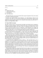
Figure 5.10:
Position rrors after completion of the bidirectional square-path
experiment (4 x 4 m).
Before calibration: b = 340.00 mm,
D
/
D
= 1.00000.
RL
After calibration: b = 336.17,
D
/
D
= 1.00084.
RL
(5.14)
(5.15)
so that
where, per definition of Equation (5.2)

Once E and E are computed, it is straightforward to use their values as compensation factors
bd
in the controller software [see Borenstein and Feng, 1995a; 1995b]. The result is a 10- to 20-fold
reduction in systematic errors.
Figure 5.10 shows the result of a typical calibration session. D and D are the effective wheel
RL
diameters, and b is the effective wheelbase.
Chapter 5: Dead-Reckoning 143
This calibration procedure can be performed with nothing more than an ordinary tape measure.
It takes about two hours to run the complete calibration procedure and measure the individual return
errors with a tape measure.
5.3.2 Reducing Non-Systematic Odometry Errors
This section introduces methods for the reduction of non-systematic odometry errors. The methods
discussed in Section 5.3.2.2 may at first confuse the reader because they were implemented on the
somewhat complex experimental platform described in Section 1.3.7. However, the methods of
Section 5.3.2.2 can be applied to many other kinematic configurations, and efforts in that direction
are subject of currently ongoing research at the University of Michigan.
5.3.2.1 Mutual Referencing
Sugiyama [1993] proposed to use two robots that could measure their positions mutually. When one
of the robots moves to another place, the other remains still, observes the motion, and determines
the first robot's new position. In other words, at any time one robot localizes itself with reference to
a fixed object: the standing robot. However, this stop and go approach limits the efficiency of the
robots.
5.3.2.2 Internal Position Error Correction
A unique way for reducing odometry errors even further is Internal Position Error Correction
(IPEC). With this approach two mobile robots mutually correct their odometry errors. However,
unlike the approach described in Section 5.3.2.1, the IPEC method works while both robots are in
continuous, fast motion [Borenstein, 1994a]. To implement this method, it is required that both
robots can measure their relative distance and bearing continuously and accurately. Coincidentally,
the MDOF vehicle with compliant linkage (described in Sec. 1.3.7) offers exactly these features, and

the IPEC method was therefore implemented and demonstrated on that MDOF vehicle. This
implementation is named Compliant Linkage Autonomous Platform with Position Error Recovery
(CLAPPER).
The CLAPPER's compliant linkage instrumentation was illustrated in Chapter 1, Figure 1.15. This
setup provides real-time feedback on the relative position and orientation of the two trucks. An
absolute encoder at each end measures the rotation of each truck (with respect to the linkage) with
a resolution of 0.3 degrees, while a linear encoder is used to measure the separation distance to
within 5 millimeters (0.2 in). Each truck computes its own dead-reckoned position and heading in
conventional fashion, based on displacement and velocity information derived from its left and right
drive-wheel encoders. By examining the perceived odometry solutions of the two robot platforms
in conjunction with their known relative orientations, the CLAPPER system can detect and
significantly reduce heading errors for both trucks (see video clip in [Borenstein, 1995V].)
The principle of operation is based on the concept of error growth rate presented by Borenstein
[1994a, 1995a], who makes a distinction between “fast-growing” and “slow-growing” odometry
errors. For example, when a differentially steered robot traverses a floor irregularity it will
immediately experience an appreciable orientation error (i.e., a fast-growing error). The associated
lateral displacement error, however, is initially very small (i.e., a slow-growing error), but grows in
an unbounded fashion as a consequence of the orientation error. The internal error correction
algorithm performs relative position measurements with a sufficiently fast update rate (20 ms) to
Lateral displacement
at end of sampling interval
a
\book\clap41.ds4; .wmf, 07/19/95
Curved path
while traversing
bump
Straight path after
traversing
bump
Center

Truck A expects
to "see" Truck B
along this line
m
Truck A actually

"sees" Truck B
along this line
lat,c
e
a
m
lat,d
144 Part II Systems and Methods for Mobile Robot Positioning
Figure 5.11:
After traversing a bump, the resulting
change of orientation of Truck A can be measured relative
to Truck B.
allow each truck to detect
fast-growing
errors in orientation, while relying on the fact that the lateral
position errors accrued by both platforms during the sampling interval were small.
Figure 5.11 explains how this method works. After traversing a bump Truck A's orientation will
change (a fact unknown to Truck A's odometry computation). Truck A is therefore expecting to
“see” Truck B along the extension of line
L
. However, because of the physically incurred rotation
e
of Truck A, the absolute encoder on truck A will report that truck B is now
actually

seen along line
L
. The angular difference between
L
and
me
L
is the thus measured odometry orientation
m
error of Truck A, which can be corrected
immediately. One should note that even if
Truck B encountered a bump at the same
time, the resulting rotation of Truck B would
not affect the orientation error measurement.
The compliant linkage in essence forms a
pseudo-stable heading reference in world
coordinates, its own orientation being dic-
tated solely by the relative translations of its
end points, which in turn are affected only
by the lateral displacements of the two
trucks. Since the lateral displacements are
slow growing
, the linkage rotates only a very
small amount between encoder samples. The
fast-growing
azimuthal disturbances of the
trucks, on the other hand, are not coupled
through the rotational joints to the linkage,
thus allowing the rotary encoders to detect
and quantify the instantaneous orientation

errors of the trucks, even when both are in
motion. Borenstein [1994a; 1995a] provides
a more complete description of this innova-
tive concept and reports experimental results
indicating improved odometry performance
of up to two orders of magnitude over con-
ventional mobile robots.
It should be noted that the rather complex
kinematic design of the MDOF vehicle is not
necessary to implement the IPEC error
correction method. Rather, the MDOF vehi-
cle happened to be available at the time and
allowed the University of Michigan research-
ers to implement and verify the validity of
the IPEC approach. Currently, efforts are
under way to implement the IPEC method
on a tractor-trailer assembly, called “
Smart
Encoder Trailer
” (SET), which is shown in
Figure 5.12. The principle of operation is
Lateral displacement
at end of sampling interval
a
Curved path
while traversing
bump
Straight path after
traversing
bump

m
lat,c
e
m
lat,d
Robot expects
to "see" trailer
along this line
Robot actual ly

"sees" trailer
along this line
\book\tvin4set.ds4; .wmf, 07/19/95
Chapter 5: Dead-Reckoning 145
Figure 5.12:
The University of Michigan's “
Smart Encoder
Trailer
” (SET) is currently being instrumented to allow the
implementation of the IPEC error correction method explained in
Section 5.3.2.2. (Courtesy of The University of Michigan.)
Figure 5.13:
Proposed implementation of
the IPEC method on a tractor-trailer
assembly.
illustrated in Figure 5.13. Simulation results, indicating
the feasibility of implementing the IPEC method on a
tractor-trailer assembly, were presented in [Borenstein,
1994b].
5.4 Inertial Navigation

An alternative method for enhancing dead reckoning is
inertial navigation, initially developed for deployment on
aircraft. The technology was quickly adapted for use on
missiles and in outer space, and found its way to mari-
time usage when the nuclear submarines
Nautilus
and
Skate
were suitably equipped in support of their transpo-
lar voyages in 1958 [Dunlap and Shufeldt, 1972]. The
principle of operation involves continuous sensing of minute accelerations in each of the three
directional axes and integrating over time to derive velocity and position. A gyroscopically stabilized
sensor platform is used to maintain consistent orientation of the three accelerometers throughout this
process.
Although fairly simple in concept, the specifics of implementation are rather demanding. This is
mainly caused by error sources that adversely affect the stability of the gyros used to ensure correct
attitude. The resulting high manufacturing and maintenance costs have effectively precluded any
practical application of this technology in the automated guided vehicle industry [Turpin, 1986]. For
example, a high-quality
inertial navigation

system
(INS) such as would be found in a commercial
airliner will have a typical drift of about 1850 meters (1 nautical mile) per hour of operation, and cost
between $50K and $70K [Byrne et al., 1992]. High-end INS packages used in ground applications
have shown performance of better than 0.1 percent of distance traveled, but cost in the neighbor-
hood of $100K to $200K, while lower performance versions (i.e., one percent of distance traveled)
run between $20K to $50K [Dahlin and Krantz, 1988].
146 Part II Systems and Methods for Mobile Robot Positioning
Experimental results from the Université Montpellier in France [Vaganay et al., 1993a; 1993b],

from the University of Oxford in the U.K. [Barshan and Durrant-Whyte, 1993; 1995], and from the
University of Michigan indicate that a purely inertial navigation approach is not realistically
advantageous (i.e., too expensive) for mobile robot applications. As a consequence, the use of INS
hardware in robotics applications to date has been generally limited to scenarios that aren’t readily
addressable by more practical alternatives. An example of such a situation is presented by Sammarco
[1990; 1994], who reports preliminary results in the case of an INS used to control an autonomous
vehicle in a mining application.
Inertial navigation is attractive mainly because it is self-contained and no external motion
information is needed for positioning. One important advantage of inertial navigation is its ability to
provide fast, low-latency dynamic measurements. Furthermore, inertial navigation sensors typically
have noise and error sources that are independent from the external sensors [Parish and Grabbe,
1993]. For example, the noise and error from an inertial navigation system should be quite different
from that of, say, a landmark-based system. Inertial navigation sensors are self-contained, non-
radiating, and non-jammable. Fundamentally, gyros provide angular rate and accelerometers provide
velocity rate information. Dynamic information is provided through direct measurements. However,
the main disadvantage is that the angular rate data and the linear velocity rate data must be
integrated once and twice (respectively), to provide orientation and linear position, respectively.
Thus, even very small errors in the rate information can cause an unbounded growth in the error of
integrated measurements. As we remarked in Section 2.2, the price of very accurate laser gyros and
optical fiber gyros have come down significantly. With price tags of $1,000 to $5,000, these devices
have now become more suitable for many mobile robot applications.
5.4.1 Accelerometers
The suitability of accelerometers for mobile robot positioning was evaluated at the University of
Michigan. In this informal study it was found that there is a very poor signal-to-noise ratio at lower
accelerations (i.e., during low-speed turns). Accelerometers also suffer from extensive drift, and they
are sensitive to uneven grounds, because any disturbance from a perfectly horizontal position will
cause the sensor to detect the gravitational acceleration g. One low-cost inertial navigation system
aimed at overcoming the latter problem included a tilt sensor [Barshan and Durrant-Whyte, 1993;
1995]. The tilt information provided by the tilt sensor was supplied to the accelerometer to cancel
the gravity component projecting on each axis of the accelerometer. Nonetheless, the results

obtained from the tilt-compensated system indicate a position drift rate of 1 to 8 cm/s (0.4 to 3.1
in/s), depending on the frequency of acceleration changes. This is an unacceptable error rate for
most mobile robot applications.
5.4.2 Gyros
Gyros have long been used in robots to augment the sometimes erroneous dead-reckoning
information of mobile robots. As we explained in Chapter 2, mechanical gyros are either inhibitively
expensive for mobile robot applications, or they have too much drift. Recent work by Barshan and
Durrant-Whyte [1993; 1994; 1995] aimed at developing an INS based on solid-state gyros, and a
fiber-optic gyro was tested by Komoriya and Oyama [1994].
0 /s
Chapter 5: Dead-Reckoning 147
Figure 5.14: Angular rate (top) and orientation (bottom) for zero-input case (i.e., gyro
remains stationary) of the
START
gyro (left) and the
Gyrostar
(right) when the bias
error is negative. The erroneous observations (due mostly to drift) are shown as the
thin line, while the EKF output, which compensates for the error, is shown as the
heavy line. (Adapted from [Barshan and Durrant-Whyte, 1995] © IEEE 1995.)
5.4.2.1 Barshan and Durrant-Whyte [1993; 1994; 1995]
Barshan and Durrant-Whyte developed a sophisticated INS using two solid-state gyros, a solid-state
triaxial accelerometer, and a two-axis tilt sensor. The cost of the complete system was £5,000
(roughly $8,000). Two different gyros were evaluated in this work. One was the ENV-O5S Gyrostar
from [MURATA], and the other was the S
olid State Angular Rate Transducer (START) gyroscope
manufactured by [GEC]. Barshan and Durrant-Whyte evaluated the performance of these two gyros
and found that they suffered relatively large drift, on the order of 5 to 15 /min. The Oxford
researchers then developed a sophisticated error model for the gyros, which was subsequently used
in an Extended Kalman Filter (EKF — see Appendix A). Figure 5.14 shows the results of the

experiment for the START gyro (left-hand side) and the Gyrostar (right-hand side). The thin plotted
lines represent the raw output from the gyros, while the thick plotted lines show the output after
conditioning the raw data in the EKF.
The two upper plots in Figure 5.14 show the measurement noise of the two gyros while they were
stationary (i.e., the rotational rate input was zero, and the gyros should ideally show ).
Barshan and Durrant-Whyte determined that the standard deviation, here used as a measure for the
148 Part II Systems and Methods for Mobile Robot Positioning
Figure 5.15: Computer simulation of a mobile robot run (Adapted from [Komoriya and Oyama, 1994].)
a. Only odometry, without gyro information. b. Odometry and gyro information fused.
amount of noise, was 0.16 /s for the START gyro and 0.24 /s for the Gyrostar. The drift in the rate
output, 10 minutes after switching on, is rated at 1.35 /s for the Gyrostar (drift-rate data for the
START was not given).
The more interesting result from the experiment in Figure 5.14 is the drift in the angular output,
shown in the lower two plots. We recall that in most mobile robot applications one is interested in
the heading of the robot, not the rate of change in the heading. The measured rate must thus be
integrated to obtain . After integration, any small constant bias in the rate measurement turns into
a constant-slope, unbounded error, as shown clearly in the lower two plots of Figure 5.14. At the end
of the five-minute experiment, the START had accumulated a heading error of -70.8 degrees while
that of the Gyrostar was -59 degrees (see thin lines in Figure 5.14). However, with the EKF, the
accumulated errors were much smaller: 12 degrees was the maximum heading error for the START
gyro, while that of the Gyrostar was -3.8 degrees.
Overall, the results from applying the EKF show a five- to six-fold reduction in the angular
measurement after a five-minute test period. However, even with the EKF, a drift rate of 1 to 3 /min
o
can still be expected.
5.4.2.2 Komoriya and Oyama [1994]
Komoriya and Oyama [1994] conducted a study of a system that uses an optical fiber gyroscope, in
conjunction with odometry information, to improve the overall accuracy of position estimation. This
fusion of information from two different sensor systems is realized through a Kalman filter (see
Appendix A).

Figure 5.15 shows a computer simulation of a path-following study without (Figure 5.15a) and
with (Figure 5.15b) the fusion of gyro information. The ellipses show the reliability of position
estimates (the probability that the robot stays within the ellipses at each estimated position is 90
percent in this simulation).
Chapter 5: Dead-Reckoning 149
Figure 5.16:
Melboy
, the mobile robot used by
Komoriya and Oyama for fusing odometry and gyro
data. (Courtesy of [Komoriya and Oyama, 1994].)
In order to test the effectiveness of their method,
Komoriya and Oyama also conducted actual
experiments with Melboy, the mobile robot shown
in Figure 5.16. In one set of experiments Melboy
was instructed to follow the path shown in
Figure 5.17a. Melboy's maximum speed was
0.14 m/s (0.5 ft/s) and that speed was further
reduced at the corners of the path in Figure 5.17a.
The final position errors without and with gyro
information are compared and shown in
Figure 5.17b for 20 runs. Figure 5.17b shows that
the deviation of the position estimation errors from
the mean value is smaller in the case where the
gyro data was used (note that a large average
deviation from the mean value indicates larger
non-systematic errors, as explained in Sec. 5.1).
Komoriya and Oyama explain that the noticeable
deviation of the mean values from the origin in
both cases could be reduced by careful calibration
of the systematic errors (see Sec. 5.3) of the mobile

robot.
We should note that from the description of this
experiment in [Komoriya and Oyama, 1994] it is
not immediately evident how the “position estima-
tion error” (i.e., the circles) in Figure 5.17b was
found. In our opinion, these points should have
been measured by marking the return position of
the robot on the floor (or by any equivalent
method that records the absolute position of the
robot and compares it with the internally computed position estimation). The results of the plot in
Figure 5.17b, however, appear to be too accurate for the absolute position error of the robot. In our
experience an error on the order of several centimeters, not millimeters, should be expected after
completing the path of Figure 5.17a (see, for example, [Borenstein and Koren, 1987; Borenstein and
Feng, 1995a; Russel, 1995].) Therefore, we interpret the data in Figure 5.17b as showing a position
error that was computed by the onboard computer, but not measured absolutely.
5.5 Summary
Odometry is a central part of almost all mobile robot navigation systems.
Improvements in odometry techniques will not change their incremental nature, i.e., even for
improved odometry, periodic absolute position updates are necessary.
150 Part II Systems and Methods for Mobile Robot Positioning
Figure 5.17: Experimental results from
Melboy
using odometry with and without a fiber-optic gyro.
a. Actual trajectory of the robot for a triangular path.
b. Position estimation errors of the robot after completing the path of a. Black circles show the errors
without gyro; white circles show the errors with the gyro.
(Adapted from [Komoriya and Oyama, 1994].)
More accurate odometry will reduce the requirements on absolute position updates and will
facilitate the solution of landmark and map-based positioning.
Inertial navigation systems alone are generally inadequate for periods of time that exceed a few

minutes. However, inertial navigation can provide accurate short-term information, for example
orientation changes during a robot maneuver. Software compensation, usually by means of a
Kalman filter, can significantly improve heading measurement accuracy.
o
0
S
\book\course9.ds4; .wmf 07/19/95
S
S
Robot
orientation
(unknown)
Figure 6.1:
The basic triangulation problem: a rotating sensor
head measures the three angles , , and between the
12 3
vehicle's longitudinal axes and the three sources S , S , and S .
12 3
C
HAPTER
6
A
CTIVE
B
EACON
N
AVIGATION
S
YSTEMS
Active beacon navigation systems are the most common navigation aids on ships and airplanes.

Active beacons can be detected reliably and provide very accurate positioning information with
minimal processing. As a result, this approach allows high sampling rates and yields high reliability,
but it does also incur high cost in installation and maintenance. Accurate mounting of beacons is
required for accurate positioning. For example, land surveyors' instruments are frequently used to
install beacons in a high-accuracy application [Maddox, 1994]. Kleeman [1992] notes that:
"Although special beacons are at odds with notions of complete robot autonomy in an
unstructured environment, they offer advantages of accuracy, simplicity, and speed - factors
of interest in industrial and office applications, where the environment can be partially
structured."
One can distinguish between two different types of active beacon systems: trilateration and
triangulation.
Trilateration
Trilateration is the determination of a vehicle's position based on distance measurements to known
beacon sources. In trilateration navigation systems there are usually three or more transmitters
mounted at known locations in the environment and one receiver on board the robot. Conversely,
there may be one transmitter on board and the receivers are mounted on the walls. Using time-of-
flight information, the system computes the distance between the stationary transmitters and the
onboard receiver. Global Positioning Systems (GPS), discussed in Section 3.1, are an example of
trilateration. Beacon systems based on ultrasonic sensors (see Sec. 6.2, below) are another example.
152 Part II Systems and Methods for Mobile Robot Positioning
Triangulation
In this configuration there are three or more active transmitters (usually infrared) mounted at known
locations in the environment, as shown in Figure 6.1. A rotating sensor on board the robot registers
the angles , , and at which it “sees” the transmitter beacons relative to the vehicle's
12 3
longitudinal axis. From these three measurements the unknown x- and y- coordinates and the
unknown vehicle orientation can be computed. Simple navigation systems of this kind can be built
very inexpensively [Borenstein and Koren, 1986]. One problem with this configuration is that the
active beacons need to be extremely powerful to insure omnidirectional transmission over large
distances. Since such powerful beacons are not very practical it is necessary to focus the beacon

within a cone-shaped propagation pattern. As a result, beacons are not visible in many areas, a
problem that is particularly grave because at least three beacons must be visible for triangulation.
A commercially available sensor system based on this configuration (manufactured and marketed
by Denning) was tested at the University of Michigan in 1990. The system provided an accuracy of
approximately ±5 centimeters (±2 in), but the aforementioned limits on the area of application made
the system unsuitable for precise navigation in large open areas.
Triangulation methods can further be distinguished by the specifics of their implementation:
a. Rotating Transmitter-Receiver, Stationary Reflectors In this implementation there is one
rotating laser beam on board the vehicle and three or more stationary retroreflectors are mounted
at known locations in the environment.
b. Rotating Transmitter, Stationary Receivers Here the transmitter, usually a rotating laser beam,
is used on board the vehicle. Three or more stationary receivers are mounted on the walls. The
receivers register the incident beam, which may also carry the encoded azimuth of the transmitter.
For either one of the above methods, we will refer to the stationary devices as “beacons,” even
though they may physically be receivers, retroreflectors, or transponders.
6.1 Discussion on Triangulation Methods
Most of the active beacon positioning systems discussed in Section 6.3 below include computers
capable of computing the vehicle's position. One typical algorithm used for this computation is
described in [Shoval et al., 1995], but most such algorithms are proprietary because the solutions are
non-trivial. In this section we discuss some aspects of triangulation algorithms.
In general, it can be shown that triangulation is sensitive to small angular errors when either the
observed angles are small, or when the observation point is on or near a circle which contains the
three beacons. Assuming reasonable angular measurement tolerances, it was found that accurate
navigation is possible throughout a large area, although error sensitivity is a function of the point of
observation and the beacon arrangements [McGillem and Rappaport, 1988].
6.1.1 Three-Point Triangulation
Cohen and Koss [1992] performed a detailed analysis on three-point triangulation algorithms and
ran computer simulations to verify the performance of different algorithms. The results are
summarized as follows:
Chapter 6: Active Beacon Navigation Systems 153

Figure 6.2: Simulation results using the algorithm
Position Estimator
on an input of noisy angle
measurements. The squared error in the position
estimate
p
(in meters) is shown as a function of
measurement errors (in percent of the actual angle).
(Reproduced and adapted with permission from [Betke
and Gurvits, 1994].)
The geometric triangulation method works consistently only when the robot is within the triangle
formed by the three beacons. There are areas outside the beacon triangle where the geometric
approach works, but these areas are difficult to determine and are highly dependent on how the
angles are defined.
The Geometric Circle Intersection method has large errors when the three beacons and the robot
all lie on, or close to, the same circle.
The Newton-Raphson method fails when the initial guess of the robot' position and orientation is
beyond a certain bound.
The heading of at least two of the beacons was required to be greater than 90 degrees. The
angular separation between any pair of beacons was required to be greater than 45 degrees.
In summary, it appears that none of the above methods alone is always suitable, but an intelligent
combination of two or more methods helps overcome the individual weaknesses.
Yet another variation of the triangulation method is the so-called running fix, proposed by Case
[1986]. The underlying principle of the running fix is that an angle or range obtained from a beacon
at time t-1 can be utilized at time t, as long as the cumulative movement vector recorded since the
reading was obtained is added to the position vector of the beacon, thus creating a virtual beacon.
6.1.2 Triangulation with More Than Three Landmarks
Betke and Gurvits [1994] developed an algorithm, called the Position Estimator, that solves the
general triangulation problem. This problem is defined as follows: given the global position of n
landmarks and corresponding angle measurements, estimate the position of the robot in the global

coordinate system. Betke and Gurvits represent the n landmarks as complex numbers and formulate
the problem as a set of linear equations. By contrast, the traditional law-of-cosines approach yields
a set of non-linear equations. Betke and Gurvits also prove mathematically that their algorithm only
fails when all landmarks are on a circle or a straight line. The algorithm estimates the robot’s position
in O(n) operations where n is the number of landmarks on a two-dimensional map.
Compared to other triangulation methods,
the Position Estimator algorithm has the fol-
lowing advantages: (1) the problem of deter-
mining the robot position in a noisy environ-
ment is linearized, (2) the algorithm runs in an
amount of time that is a linear function of the
number of landmarks, (3) the algorithm pro-
vides a position estimate that is close to the
actual robot position, and (4) large errors (“out-
liers”) can be found and corrected.
Betke and Gurvits present results of a simu-
lation for the following scenario: the robot is at
the origin of the map, and the landmarks are
randomly distributed in a 10×10 meter
(32×32 ft) area (see Fig. 6.2). The robot is at
the corner of this area. The distance between a
landmark and the robot is at most 14.1 meters
154 Part II Systems and Methods for Mobile Robot Positioning
Figure 6.3: Simulation results showing the effect
of outliers and the result of removing the outliers.
(Reproduced and adapted with permission from
[Betke and Gurvits, 1994].)
(46 ft) and the angles are at most 45 degrees. The
simulation results show that large errors due to
misidentified landmarks and erroneous angle mea-

surements can be found and discarded. Subse-
quently, the algorithm can be repeated without the
outliers, yielding improved results. One example is
shown in Figure 6.3, which depicts simulation results
using the algorithm Position Estimator. The algo-
rithm works on an input of 20 landmarks (not shown
in Figure 6.3) that were randomly placed in a 10×10
meters (32×32 ft) workspace. The simulated robot is
located at (0, 0). Eighteen of the landmarks were
simulated to have a one-percent error in the angle
measurement and two of the landmarks were simu-
lated to have a large 10-percent angle measurement
error. With the angle measurements from 20 land-
marks the Position Estimator produces 19 position estimates p - p (shown as small blobs in
119
Figure 6.3). Averaging these 19 estimates yields the computed robot position. Because of the two
landmarks with large angle measurement errors two position estimates are bad: p at (79 cm, 72 cm)
5
and p at (12.5 cm, 18.3 cm). Because of these poor position estimates, the resulting centroid
18
(average) is at P = (17 cm, 24 cm). However, the Position Estimator can identify and exclude the
a
two outliers. The centroid calculated without the outliers p and p is at P = (12.5 cm, 18.3 cm). The
518
b
final position estimate after the Position Estimator is applied again on the 18 “good” landmarks (i.e.,
without the two outliers) is at P = (6.5 cm, 6.5 cm).
c
6.2 Ultrasonic Transponder Trilateration
Ultrasonic trilateration schemes offer a medium- to high-accuracy, low-cost solution to the position

location problem for mobile robots. Because of the relatively short range of ultrasound, these
systems are suitable for operation in relatively small work areas and only if no significant
obstructions are present to interfere with wave propagation. The advantages of a system of this type
fall off rapidly, however, in large multi-room facilities due to the significant complexity associated
with installing multiple networked beacons throughout the operating area.
Two general implementations exist: 1) a single transducer transmitting from the robot, with
multiple fixed-location receivers, and 2) a single receiver listening on the robot, with multiple fixed
transmitters serving as beacons. The first of these categories is probably better suited to applications
involving only one or at most a very small number of robots, whereas the latter case is basically
unaffected by the number of passive receiver platforms involved (i.e., somewhat analogous to the
Navstar GPS concept).
Pinger side
view
pinger
"A"
Base station
pinger
"B"
Chapter 6: Active Beacon Navigation Systems 155
Figure 6.4: The ISR Genghis series of legged robots localize x-y
position with a master/slave trilateration scheme using two 40 kHz
ultrasonic “pingers.” (Adapted from [ISR, 1994].)
6.2.1 IS Robotics 2-D Location System
IS Robotics, Inc. [ISR], Somerville, MA, a spin-off company from MIT's renowned Mobile Robotics
Lab, has introduced a beacon system based on an inexpensive ultrasonic trilateration system. This
system allows their Genghis series robots to localize position to within 12.7 millimeters (0.5 in) over
a 9.1×9.1 meter (30×30 ft) operating area [ISR, 1994]. The ISR system consists of a base station
master hard-wired to two slave ultrasonic “pingers” positioned a known distance apart (typically 2.28
m — 90 in) along the edge of the operating area as shown in Figure 6.4. Each robot is equipped with
a receiving ultrasonic transducer situated beneath a cone-shaped reflector for omnidirectional

coverage. Communication between the base station and individual robots is accomplished using a
Proxim spread-spectrum (902 to 928 MHz) RF link.
The base station alternately
fires the two 40-kHz ultrasonic
pingers every half second, each
time transmitting a two-byte
radio packet in broadcast mode
to advise all robots of pulse
emission. Elapsed time between
radio packet reception and de-
tection of the ultrasonic wave
front is used to calculate dis-
tance between the robot’s cur-
rent position and the known
location of the active beacon.
Inter-robot communication is
accomplished over the same
spread-spectrum channel using a
time-division-multiple-access
scheme controlled by the base
station. Principle sources of er-
ror include variations in the speed of sound, the finite size of the ultrasonic transducers, non-repetitive
propagation delays in the electronics, and ambiguities associated with time-of-arrival detection. The
cost for this system is $10,000.
6.2.2 Tulane University 3-D Location System
Researchers at Tulane University in New Orleans, LA, have come up with some interesting methods
for significantly improving the time-of-arrival measurement accuracy for ultrasonic transmitter-
receiver configurations, as well as compensating for the varying effects of temperature and humidity.
In the hybrid scheme illustrated in Figure 6.5, envelope peak detection is employed to establish the
approximate time of signal arrival, and to consequently eliminate ambiguity interval problems for a

more precise phase-measurement technique that provides final resolution [Figueroa and Lamancusa,
1992]. The desired 0.025 millimeters (0.001 in) range accuracy required a time unit discrimination
of 75 nanoseconds at the receiver, which can easily be achieved using fairly simplistic phase
measurement circuitry, but only within the interval of a single wavelength. The actual distance from
transmitter to receiver is the summation of some integer number of wavelengths (determined by the
Phase detection
Digital I/O
in PC
Envelope of squared wave TOF
Rough
From
receiver
End of
RTOF
TTL of received waveform
Amplified waveform
40 kHz reference
differentiationAfter
Phase
difference
( )
( )
*
*
*
( )
*
*
*
t t

t t
t t
r x y z
r x y z
r x y z
p
c
c
u
c
v
c
w
c
d
d
n d n n n n
1
2
2
2
2
1
2
1 1 1
2
2
2 2 2
2
2

2
2
2
2
2
1 2 2 2
1 2 2 2
1 2 2 2
1
−
−
−























=




















−
−
−































156 Part II Systems and Methods for Mobile Robot Positioning
Figure 6.5: A combination of threshold adjusting and phase detection is employed to provide higher

accuracy in time-of-arrival measurements in the Tulane University ultrasonic position-location system
[Figueroa and Lamancusa, 1992].
(6.1)
coarse time-of-arrival measurement) plus that fractional portion of a wavelength represented by the
phase measurement results.
Details of this time-of-arrival detection scheme and associated error sources are presented by
Figueroa and Lamancusa [1992]. Range measurement accuracy of the prototype system was
experimentally determined to be 0.15 millimeters (0.006 in) using both threshold adjustments (based
on peak detection) and phase correction, as compared to 0.53 millimeters (0.021 in) for threshold
adjustment alone. These high-accuracy requirements were necessary for an application that involved
tracking the end-effector of a 6-DOF industrial robot [Figueroa et al, 1992]. The system incorporates
seven 90-degree Massa piezoelectric transducers operating at 40 kHz, interfaced to a 33 MHz IBM-
compatible PC. The general position-location strategy was based on a trilateration method developed
by Figueroa and Mohegan [1994].
The set of equations describing time-of-flight measurements for an ultrasonic pulse propagating
from a mobile transmitter located at point (u, v, w) to various receivers fixed in the inertial reference
frame can be listed in matrix form as follows [Figueroa and Mohegan, 1994]:
Chapter 6: Active Beacon Navigation Systems 157
where:
t = measured time of flight for transmitted pulse to reach i receiver
i
th
t = system throughput delay constant
d
r = sum of squares of i receiver coordinates
i
2 th
(x, y, z) = location coordinates of i receiver
iii
th

(u, v, w) = location coordinates of mobile transmitter
c = speed of sound
p = sum of squares of transmitter coordinates.
2
The above equation can be solved for the vector on the right to yield an estimated solution for
the speed of sound c, transmitter coordinates (u, v, w), and an independent term p that can be
2
compared to the sum of the squares of the transmitter coordinates as a checksum indicator [Figueroa
and Mahajan, 1994]. An important feature of this representation is the use of an additional receiver
(and associated equation) to enable treatment of the speed of sound itself as an unknown, thus
ensuring continuous on-the-fly recalibration to account for temperature and humidity effects. (The
system throughput delay constant t can also be determined automatically from a pair of equations
d
for 1/c using two known transmitter positions. This procedure yields two equations with t and c as
2
d
unknowns, assuming c remains constant during the procedure.) A minimum of five receivers is
required for an unambiguous three-dimensional position solution, but more can be employed to
achieve higher accuracy using a least-squares estimation approach. Care must be taken in the
placement of receivers to avoid singularities as defined by Mahajan [1992].
Figueroa and Mahajan [1994] report a follow-up version intended for mobile robot positioning
that achieves 0.25 millimeters (0.01 in) accuracy with an update rate of 100 Hz. The prototype
system tracks a TRC LabMate over a 2.7×3.7 meter (9×12 ft) operating area with five ceiling-
mounted receivers and can be extended to larger floor plans with the addition of more receiver sets.
An RF link will be used to provide timing information to the receivers and to transmit the subsequent
x-y position solution back to the robot. Three problem areas are being further investigated to
increase the effective coverage and improve resolution:
Actual transmission range does not match the advertised operating range for the ultrasonic
transducers, probably due to a resonant frequency mismatch between the transducers and
electronic circuitry.

The resolution of the clocks (6 MHz) used to measure time of flight is insufficient for automatic
compensation for variations in the speed of sound.
The phase-detection range-measurement correction sometimes fails when there is more than one
wavelength of uncertainty. This problem can likely be solved using the frequency division scheme
described by Figueroa and Barbieri [1991].
6.3 Optical Positioning Systems
Optical positioning systems typically involve some type of scanning mechanism operating in
conjunction with fixed-location references strategically placed at predefined locations within the
operating environment. A number of variations on this theme are seen in practice [Everett, 1995]:
Right zone
Left zone
Docking
Optical beacon
head
beacon
controller
Optical axis
Sonar transmitter
Beacon sensor
B
Sonar receiver
158 Part II Systems and Methods for Mobile Robot Positioning
Figure 6.6
: The structured-light near-infrared beacon on the
Cybermotion battery recharging station defines an optimal path of
approach for the
K2A Navmaster
robot [Everett, 1995].
Scanning detectors with fixed active beacon emitters.
Scanning emitter/detectors with passive retroreflective targets.

Scanning emitter/detectors with active transponder targets.
Rotating emitters with fixed detector targets.
One of the principal problems associated with optical beacon systems, aside from the obvious
requirement to modify the environment, is the need to preserve a clear line of sight between the
robot and the beacon. Preserving an unobstructed view is sometimes difficult if not impossible in
certain applications such as congested warehouse environments. In the case of passive retro-
reflective targets, problems can sometimes arise from unwanted returns from other reflective
surfaces in the surrounding environment, but a number of techniques exists for minimizing such
interference.
6.3.1 Cybermotion Docking Beacon
The automated docking system used on the Cybermotion Navmaster robot incorporates the unique
combination of a structured-light beacon (to establish bearing) along with a one-way ultrasonic
ranging system (to determine standoff distance). The optical portion consists of a pair of near-
infrared transceiver units, one mounted on the front of the robot and the other situated in a known
position and orientation within the operating environment. These two optical transceivers are capable
of full-duplex data transfer between the robot and the dock at a rate of 9600 bits per second.
Separate modulation frequencies of 154 and 205 kHz are employed for the uplink and downlink
respectively to eliminate crosstalk. Under normal circumstances, the dock-mounted transceiver waits
passively until interrogated by an active transmission from the robot. If the interrogation is
specifically addressed to the assigned ID number for that particular dock, the dock control computer
activates the beacon transmitter for 20 seconds. (Dock IDs are jumper selectable at time of
installation.)
Figure 6.6 shows the fixed-location
beacon illuminating a 90-degree field
of regard broken up into two uniquely
identified zones, designated for pur-
poses of illustration here as the Left
Zone and Right Zone. An array of
LED emitters in the beacon head is
divided by a double-sided mirror ar-

ranged along the optical axis and a
pair of lenses. Positive zone identifica-
tion is initiated upon request from the
robot in the form of a NAV Interroga-
tion byte transmitted over the optical
datalink. LEDs on opposite sides of
the mirror respond to this NAV Inter-
rogation with slightly different coded
responses. The robot can thus deter-
mine its relative location with respect
Chapter 6: Active Beacon Navigation Systems 159
to the optical axis of the beacon based on the response bit pattern detected by the onboard receiver
circuitry.
Once the beacon starts emitting, the robot turns in the appropriate direction and executes the
steepest possible (i.e., without losing sight of the beacon) intercept angle with the beacon optical
axis. Crossing the optical axis at point B is flagged by a sudden change in the bit pattern of the NAV
Response Byte, whereupon the robot turns inward to face the dock. The beacon optical axis
establishes the nominal path of approach and in conjunction with range offset information uniquely
defines the robot’s absolute location. This situation is somewhat analogous to a TACAN station
[Dodington, 1989] but with a single defined radial.
The offset distance from vehicle to dock is determined in rather elegant fashion by a dedicated
non-reflective ultrasonic ranging configuration. This high-frequency (>200 kHz) narrow-beam (15 )
o
sonar system consists of a piezoelectric transmitter mounted on the docking beacon head and a
complimentary receiving transducer mounted on the front of the vehicle. A ranging operation is
initiated upon receipt of the NAV Interrogation Byte from the robot; the answering NAV Response
Byte from the docking beacon signals the simultaneous transmission of an ultrasonic pulse. The
difference at the robot end between time of arrival for the NAV Response Byte over the optical link
and subsequent ultrasonic pulse detection is used to calculate separation distance. This dual-
transducer master/slave technique assures an unambiguous range determination between two well

defined points and is unaffected by any projections on or around the docking beacon and/or face of
the robot.
During transmission of a NAV Interrogation Byte, the left and right sides of the LED array
located on the robot are also driven with uniquely identifiable bit patterns. This feature allows the
docking beacon computer to determine the robot’s actual heading with respect to the nominal path
of approach. Recall the docking beacon’s structured bit pattern establishes (in similar fashion) the
side of the vehicle centerline on which the docking beacon is located. This heading information is
subsequently encoded into the NAV Response Byte and passed to the robot to facilitate course
correction. The robot closes on the beacon, halting at the defined stop range (not to exceed 8 ft) as
repeatedly measured by the docking sonar. Special instructions in the path program can then be used
to reset vehicle heading and/or position.
6.3.2 Hilare
Early work incorporating passive beacon tracking at the Laboratoire d’Automatique et d’Analyse
des Systemes, Toulouse, France, involved the development of a navigation subsystem for the mobile
robot Hilare [Banzil et al., 1981]. The system consisted of two near-infrared emitter/detectors
mounted with a 25 centimeters (10 in) vertical separation on a rotating mast, used in conjunction
with passive reflective beacon arrays at known locations in three corners of the room.
Each of these beacon arrays was constructed of retroreflective tape applied to three vertical
cylinders, which were then placed in a recognizable configuration as shown in Figure 6.7. One of the
arrays was inverted so as to be uniquely distinguishable for purposes of establishing an origin. The
cylinders were vertically spaced to intersect the two planes of light generated by the rotating optical
axes of the two emitters on the robot’s mast. A detected reflection pattern as in Figure 6.8 confirmed
beacon acquisition. Angular orientation relative to each of the retroreflective arrays was inferred
from the stepper-motor commands that drove the scanning mechanism; lateral position was
determined through simple triangulation.
d
d
d
d
d

R
R
R
160 Part II Systems and Methods for Mobile Robot Positioning
Figure 6.7:
Retroreflective beacon array
configuration used on the mobile robot
Hilare
.
(Adapted from [Banzil et al, 1981].)
Figure 6.8:
A confirmed reflection pattern as depicted
above was required to eliminate potential interference
from other highly specular surfaces [Banzil et al., 1981].
Figure 6.9:
The
LASERNET
beacon tracking system.
(Courtesy of Namco Controls Corp.)
6.3.3 NAMCO LASERNET
The NAMCO LASERNET beacon tracking system (Figure 6.9) employs retroreflective targets
distributed throughout the operating area of an automated guided vehicle (AGV) in order to measure
range and angular position (Figure 6.10). A servo-controlled rotating mirror pans a near-infrared
laser beam through a horizontal arc of 90 degrees at a 20 Hz update rate. When the beam sweeps
across a target of known dimensions, a return signal of finite duration is sensed by the detector. Since
the targets are all the same size, the signal generated by a close target will be of longer duration than
that from a distant one.
Angle measurement is initiated when the
scanner begins its sweep from right to left;
the laser strikes an internal synchronization

photodetector that starts a timing sequence.
The beam is then panned across the scene
until returned by a retroreflective target in
the field of view. The reflected signal is
detected by the sensor, terminating the
timing sequence (Fig. 6.11). The elapsed
time is used to calculate the angular position
of the target in the equation [NAMCO,
1989]
= Vt - 45 (6.2)
b
where
= target angle
V = scan velocity (7,200 /s)
T = time between scan initiation and target
b
detection.