Where.Am.I-Sensors.and.methods.for.mobile.robot.positioning.-.Borenstein(2001) Part 10 pot

Chapter 7: Landmark Navigation 181
relating to, or contributing to the sense of smell (The American Heritage Dictionary of the English Language, Third Edition is
1
licensed from Houghton Mifflin Company. Copyright © 1992 by Houghton Mifflin Company. All rights reserved).
In this book we don't address these methods in detail, because they do not allow the vehicle to
move freely — the main feature that sets mobile robots apart from AGVs. However, two recently
introduced variations of the line navigation approach are of interest for mobile robots. Both
techniques are based on the use of short-lived navigational markers (SLNM). The short-lived nature
of the markers has the advantage that it is not necessary to remove the markers after use.
One typical group of applications suitable for SLNM are floor coverage applications. Examples
are floor cleaning, lawn mowing, or floor surveillance. In such applications it is important for the
robot to travel along adjacent paths on the floor, with minimal overlap and without “blank” spots.
With the methods discussed here, the robot could conceivably mark the outside border of the path,
and trace that border line in a subsequent run. One major limitation of the current state-of-the-art is
that they permit only very slow travel speeds: on the order of under 10 mm/s (0.4 in/s).
7.4.1 Thermal Navigational Marker
Kleeman [1992], Kleeman and Russell [1993], and Russell [1993] report on a pyroelectric sensor that
has been developed to detect thermal paths created by heating the floor with a quartz halogen bulb.
The path is detected by a pyroelectric sensor based on lithium-tantalate. In order to generate a
differential signal required for path following, the position of a single pyroelectric sensor is toggled
between two sensing locations 5 centimeters (2 in) apart. An aluminum enclosure screens the sensor
from ambient infrared light and electromagnetic disturbances. The 70 W quartz halogen bulb used in
this system is located 30 millimeters (1-3/16 in) above the floor.
The volatile nature of this path is both advantageous and disadvantageous: since the heat trail
disappears after a few minutes, it also becomes more difficult to detect over time. Kleeman and
Russell approximated the temperature distribution T at a distance d from the trail and at a time t after
laying the trail as
T(d,t) = A(t) e (7.2)
-(d/w)²
where A(t) is a time-variant intensity function of the thermal path.
In a controlled experiment two robots were used. One robot laid the thermal path at a speed of

10 mm/s (0.4 in/s), and the other robot followed that path at about the same speed. Using a control
scheme based on a Kalman filter, thermal paths could be tracked up to 10 minutes after being laid on
a vinyl tiled floor. Kleeman and Russell remarked that the thermal footprint of peoples' feet could
contaminate the trail and cause the robot to lose track.
7.4.2 Volatile Chemicals Navigational Marker
This interesting technique is based on laying down an odor trail and using an olfactory sensor to
1
allow a mobile robot to follow the trail at a later time. The technique was described by Deveza et al.
[1993] and Russell et al. [1994], and the experimental system was further enhanced as described by
Russell [1995a; 1995b] at Monash University in Australia. Russell's improved system comprises a
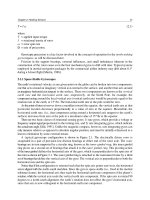
custom-built robot (see Figure 7.10) equipped with an odor-sensing system. The sensor system uses
182 Part II Systems and Methods for Mobile Robot Positioning
Figure 7.10: The odor-laying/odor-sensing mobile robot was
developed at Monash University in Australia. The olfactory
sensor is seen in front of the robot. At the top of the vertical
boom is a magnetic compass. (Courtesy of Monash
University).
Figure 7.11: Odor sensor response as the robot crosses a line of camphor set at an angle of
a. 90E and b. 20E to the robot path. The robots speed was 6 mm/s (1/4 in/s) in both tests. (Adapted
with permission from Russell [1995].)
controlled flows of air to draw odor-
laden air over a sensor crystal. The
quartz crystal is used as a sensitive
balance to weigh odor molecules. The
quartz crystal has a coating with a
specific affinity for the target odorant;
molecules of that odorant attach easily
to the coating and thereby increase the
total mass of the crystal. While the
change of mass is extremely small, it

suffices to change the resonant fre-
quency of the crystal. A 68HC11 mi-
croprocessor is used to count the crys-
tal's frequency, which is in the kHz
region. A change of frequency is indic-
ative of odor concentration. In Rus-
sell's system two such sensors are
mounted at a distance of 30 millime-
ters (1-3/16 in) from each other, to
provide a differential signal that can
then be used for path tracking.
For laying the odor trail, Russell
used a modified felt-tip pen. The odor-
laden agent is camphor, dissolved in
alcohol. When applied to the floor, the alcohol evaporates quickly and leaves a 10 millimeter (0.4 in)
wide camphor trail. Russell measured the response time of the olfactory sensor by letting the robot
cross an odor trail at angles of 90 and 20 degrees. The results of that test are shown in Figure 7.11.
Currently, the foremost limitation of Russell's volatile chemical navigational marker is the robot's slow
speed of 6 mm/s (1/4 in/s).
Chapter 7: Landmark Navigation 183
7.5 Summary
Artificial landmark detection methods are well developed and reliable. By contrast, natural
landmark navigation is not sufficiently developed yet for reliable performance under a variety of
conditions. A survey of the market of commercially available natural landmark systems produces
only a few. One is TRC's vision system that allows the robot to localize itself using rectangular and
circular ceiling lights [King and Weiman, 1990]. Cyberworks has a similar system [Cyberworks]. It
is generally very difficult to develop a feature-based landmark positioning system capable of
detecting different natural landmarks in different environments. It is also very difficult to develop
a system that is capable of using many different types of landmarks.
We summarize the characteristics of landmark-based navigation as follows:

Natural landmarks offer flexibility and require no modifications to the environment.
Artificial landmarks are inexpensive and can have additional information encoded as patterns or
shapes.
The maximal distance between robot and landmark is substantially shorter than in active beacon
systems.
The positioning accuracy depends on the distance and angle between the robot and the landmark.
Landmark navigation is rather inaccurate when the robot is further away from the landmark. A
higher degree of accuracy is obtained only when the robot is near a landmark.
Substantially more processing is necessary than with active beacon systems.
Ambient conditions, such as lighting, can be problematic; in marginal visibility, landmarks may
not be recognized at all or other objects in the environment with similar features can be mistaken
for a legitimate landmark.
Landmarks must be available in the work environment around the robot.
Landmark-based navigation requires an approximate starting location so that the robot knows
where to look for landmarks. If the starting position is not known, the robot has to conduct a time-
consuming search process.
A database of landmarks and their location in the environment must be maintained.
There is only limited commercial support for this type of technique.
Establish
correspondence
between local map
and stored global map
Figure 8.1:
General procedure for map-based positioning.
C
HAPTER
8
M
AP
-

BASED
P
OSITIONING
Map-based positioning, also known as “map matching,” is a technique in which the robot uses its
sensors to create a map of its local environment. This local map is then compared to a global map
previously stored in memory. If a match is found, then the robot can compute its actual position and
orientation in the environment. The prestored map can be a CAD model of the environment, or it
can be constructed from prior sensor data.
The basic procedure for map-based positioning is shown in Figure 8.1.
The main advantages of map-based positioning are as follows.
This method uses the naturally occurring structure of typical indoor environments to derive
position information without modifying the environment.
Map-based positioning can be used to generate an updated map of the environment. Environment
maps are important for other mobile robot tasks, such as global path planning or the avoidance
of “local minima traps” in some local obstacle avoidance methods.
Map-based positioning allows a robot to learn a new environment and to improve positioning
accuracy through exploration.
Disadvantages of map-based positioning are the specific requirements for satisfactory navigation.
For example, map-based positioning requires that:
there be enough stationary, easily distinguishable features that can be used for matching,
the sensor map be accurate enough (depending on the tasks) to be useful,
a significant amount of sensing and processing power be available.
One should note that currently most work in map-based positioning is limited to laboratory settings
and to relatively simple environments.
Chapter 8: Map-Based Positioning 185
8.1 Map Building
There are two fundamentally different starting points for the map-based positioning process. Either
there is a pre-existing map, or the robot has to build its own environment map. Rencken [1993]
defined the map building problem as the following: “Given the robot's position and a set of
measurements, what are the sensors seeing?" Obviously, the map-building ability of a robot is

closely related to its sensing capacity.
Talluri and Aggarwal [1993] explained:
"The position estimation strategies that use map-based positioning rely on the robot's
ability to sense the environment and to build a representation of it, and to use this
representation effectively and efficiently. The sensing modalities used significantly
affect the map making strategy. Error and uncertainty analyses play an important role
in accurate position estimation and map building. It is important to take explicit
account of the uncertainties; modeling the errors by probability distributions and
using Kalman filtering techniques are good ways to deal with these errors explicitly."
Talluri and Aggarwal [1993] also summarized the basic requirements for a map:
"The type of spatial representation system used by a robot should provide a way to
incorporate consistently the newly sensed information into the existing world model.
It should also provide the necessary information and procedures for estimating the
position and pose of the robot in the environment. Information to do path planning,
obstacle avoidance, and other navigation tasks must also be easily extractable from
the built world model."
Hoppen et al. [1990] listed the three main steps of sensor data processing for map building:
1. Feature extraction from raw sensor data.
2. Fusion of data from various sensor types.
3. Automatic generation of an environment model with different degrees of abstraction.
And Crowley [1989] summarized the construction and maintenance of a composite local world
model as a three-step process:
1. Building an abstract description of the most recent sensor data (a sensor model).
2. Matching and determining the correspondence between the most recent sensor models and the
current contents of the composite local model.
3. Modifying the components of the composite local model and reinforcing or decaying the
confidences to reflect the results of matching.
A problem related to map-building is “autonomous exploration.” In order to build a map, the
robot must explore its environment to map uncharted areas. Typically it is assumed that the robot
begins its exploration without having any knowledge of the environment. Then, a certain motion

strategy is followed which aims at maximizing the amount of charted area in the least amount of
m
pq
x y
x
p
y
q
G(x,y) p,q 0,1,2,
µ
pq
x y
(x x)
p
(y y)
q
G(x,y)
186 Part II Systems and Methods for Mobile Robot Positioning
(8.1)
(8.2)
time. Such a motion strategy is called exploration strategy, and it depends strongly on the kind of
sensors used. One example for a simple exploration strategy based on a lidar sensor is given by
[Edlinger and Puttkamer, 1994].
8.1.1 Map-Building and Sensor Fusion
Many researchers believe that no single sensor modality alone can adequately capture all relevant
features of a real environment. To overcome this problem, it is necessary to combine data from
different sensor modalities, a process known as sensor fusion. Here are a few examples:
Buchberger et al. [1993] and Jörg [1994; 1995] developed a mechanism that utilizes heteroge-
neous information obtained from a laser-radar and a sonar system in order to construct a reliable
and complete world model.

Courtney and Jain [1994] integrated three common sensing sources (sonar, vision, and infrared)
for sensor-based spatial representation. They implemented a feature-level approach to sensor
fusion from multisensory grid maps using a mathematical method based on spatial moments and
moment invariants, which are defined as follows:
The two-dimensional (p+q)th order spacial moments of a grid map G(x,y) are defined as
Using the centroid, translation-invariant central moments (moments don't change with the
translation of the grid map in the world coordinate system) are formulated:
From the second- and third-order central moments, a set of seven moment invariants that are
independent of translation, rotation, and scale can be derived. A more detailed treatment of spatial
moments and moment invariants is given in [Gonzalez and Wintz, 1977].
8.1.2 Phenomenological vs. Geometric Representation, Engelson and McDermott [1992]
Most research in sensor-based map building attempts to minimize mapping errors at the earliest stage
— when the sensor data is entered into the map. Engelson and McDermott [1992] suggest that this
methodology will reach a point of diminishing returns, and hence further research should focus on
explicit error detection and correction. The authors observed that the geometric approach attempts
to build a more-or-less detailed geometric description of the environment from perceptual data. This
has the intuitive advantage of having a reasonably well-defined relation to the real world. However,
there is, as yet, no truly satisfactory representation of uncertain geometry, and it is unclear whether
the volumes of information that one could potentially gather about the shape of the world are really
useful.
To overcome this problem Engelson and McDermott suggested the use of a topological approach
that constitutes a phenomenological representation of the robot's potential interactions with the
world, and so directly supports navigation planning. Positions are represented relative to local
Chapter 8: Map-Based Positioning 187
reference frames to avoid unnecessary accumulation of relative errors. Geometric relations between
frames are also explicitly represented. New reference frames are created whenever the robot's
position uncertainty grows too high; frames are merged when the uncertainty between them falls
sufficiently low. This policy ensures locally bounded uncertainty. Engelson and McDermott showed
that such error correction can be done without keeping track of all mapping decisions ever made.
The methodology makes use of the environmental structure to determine the essential information

needed to correct mapping errors. The authors also showed that it is not necessary for the decision
that caused an error to be specifically identified for the error to be corrected. It is enough that the
type of error can be identified. The approach has been implemented only in a simulated environment,
where the effectiveness of the phenomenological representation was demonstrated.
8.2 Map Matching
One of the most important and challenging aspects of map-based navigation is map matching, i.e.,
establishing the correspondence between a current local map and the stored global map [Kak et al.,
1990]. Work on map matching in the computer vision community is often focused on the general
problem of matching an image of arbitrary position and orientation relative to a model (e.g., [Talluri
and Aggarwal, 1993]). In general, matching is achieved by first extracting features, followed by
determination of the correct correspondence between image and model features, usually by some
form of constrained search [Cox, 1991].
Such matching algorithms can be classified as either icon-based or feature-based. Schaffer et al.
[1992] summarized these two approaches:
"Iconic-based pose estimation pairs sensory data points with features from the map,
based on minimum distance. The robot pose is solved for that minimizes the distance
error between the range points and their corresponding map features. The robot pose
is solved [such as to] minimize the distance error between the range points and their
corresponding map features. Based on the new pose, the correspondences are
recomputed and the process repeats until the change in aggregate distance error
between points and line segments falls below a threshold. This algorithm differs from
the feature-based method in that it matches every range data point to the map rather
than corresponding the range data into a small set of features to be matched to the
map. The feature-based estimator, in general, is faster than the iconic estimator and
does not require a good initial heading estimate. The iconic estimator can use fewer
points than the feature-based estimator, can handle less-than-ideal environments, and
is more accurate. Both estimators are robust to some error in the map."
Kak et al. [1990] pointed out that one problem in map matching is that the sensor readings and
the world model may be of different formats. One typical solution to this problem is that the
approximate position based on odometry is utilized to generate (from the prestored global model),

an estimated visual scene that would be “seen” by robot. This estimated scene is then matched
against the actual scene viewed by the onboard sensors. Once the matches are established between
the features of the two images (expected and actual), the position of the robot can be estimated with
reduced uncertainty. This approach is also supported by Rencken [1994], as will be discussed in
more detail below.
188 Part II Systems and Methods for Mobile Robot Positioning
In order to match the current sensory data to the stored environment model reliably, several
features must be used simultaneously. This is particularly true for a range image-based system since
the types of features are limited to a range image map. Long walls and edges are the most commonly
used features in a range image-based system. In general, the more features used in one match, the
less likely a mismatch will occur, but the longer it takes to process. A realistic model for the
odometry and its associated uncertainty is the basis for the proper functioning of a map-based
positioning system. This is because the feature detection as well as the updated position calculation
rely on odometric estimates [Chenavier and Crowley, 1992].

8.2.1 Schiele and Crowley [1994]
Schiele and Crowley [1994] discussed different matching techniques for matching two occupancy
grids. The first grid is the local grid that is centered on the robot and models its vicinity using the
most recent sensor readings. The second grid is a global model of the environment furnished either
by learning or by some form of computer-aided design tool. Schiele and Crowley propose that two
representations be used in environment modeling with sonars: parametric primitives and an
occupancy grid. Parametric primitives describe the limits of free space in terms of segments or
surfaces defined by a list of parameters. However, noise in the sensor signals can make the process
of grouping sensor readings to form geometric primitives unreliable. In particular, small obstacles
such as table legs are practically impossible to distinguish from noise.
Schiele and Crowley discuss four different matches:
Matching segment to segment as realized by comparing segments in (1) similarity in orientation,
(2) collinearity, and (3) overlap.
Matching segment to grid.
Matching grid to segment.

Matching grid to grid as realized by generating a mask of the local grid. This mask is then
transformed into the global grid and correlated with the global grid cells lying under this mask.
The value of that correlation increases when the cells are of the same state and decreases when
the two cells have different states. Finally finding the transformation that generates the largest
correlation value.
Schiele and Crowley pointed out the importance of designing the updating process to take into
account the uncertainty of the local grid position. The correction of the estimated position of the
robot is very important for the updating process particularly during exploration of unknown
environments.
Figure 8.2 shows an example of one of the experiments with the robot in a hallway. Experimental
results obtained by Schiele and Crowley show that the most stable position estimation results are
obtained by matching segments to segments or grids to grids.
8.2.2 Hinkel and Knieriemen [1988] — The Angle Histogram
Hinkel and Knieriemen [1988] from the University of Kaiserslautern, Germany, developed a world-
modeling method called the Angle Histogram. In their work they used an in-house developed lidar
mounted on their mobile robot Mobot III. Figure 8.3 shows that lidar system mounted on Mobot III's
Chapter 8: Map-Based Positioning 189
Figure 8.2: Schiele and Crowley's robot models its position in a hallway.
a. Raw ultrasonic range data projected onto external coordinates around the robot.
b. Local grid and the edge segments extracted from this grid.
c. The robot with its uncertainty in estimated position within the global grid.
d. The local grid imposed on the global grid at the position and orientation of best
correspondence.
(Reproduced and adapted from [Schiele and Crowley, 1994].)
successor Mobot IV. (Note that the photograph in Figure 8.3 is very recent; it shows Mobot IV on
the left, and Mobot V, which was built in 1995, on the right. Also note that an ORS-1 lidar from ESP,
discussed in Sec. 4.2.2, is mounted on Mobot V.)
A typical scan from the in-house lidar is shown in Figure 8.4. The similarity between the scan
quality of the University of Kaiserslautern lidar and that of the ORS-1 lidar (see Fig. 4.32a in
Sec. 4.2.6) is striking.

The angle histogram method works as follows. First, a 360 degree scan of the room is taken with
the lidar, and the resulting “hits” are recorded in a map. Then the algorithm measures the relative
angle between any two adjacent hits (see Figure 8.5). After compensating for noise in the readings
(caused by the inaccuracies in position between adjacent hits), the angle histogram shown in Figure
8.6a can be built. The uniform direction of the main walls are clearly visible as peaks in the angle
histogram. Computing the histogram modulo results in only two main peaks: one for each pair of
parallel walls. This algorithm is very robust with regard to openings in the walls, such as doors and
windows, or even cabinets lining the walls.
190 Part II Systems and Methods for Mobile Robot Positioning
Figure 8.3:
Mobot IV
(left) and
Mobot V
(right) were both developed and built
at the University of Kaiserslautern. The different
Mobot
models have served as
mobile robot testbeds since the mid-eighties. (Courtesy of the University of
Kaiserslautern.)
Figure 8.4: A typical scan of a room, produced by the University of
Kaiserslautern's in-house developed lidar system. (Courtesy of the
University of Kaiserslautern.)
After computing the angle histogram, all angles of the hits can be normalized, resulting in the
x
weiss00.ds4, .wmf
20
o
pos10rpt.ds4, .wmf
Chapter 8: Map-Based Positioning 191
Figure 8.5: Calculating angles for the angle histogram.

(Courtesy of [Weiß et al., 1994].)
Figure 8.6: Readings from a rotating laser scanner generate the contours of a room.
a. The angle histogram allows the robot to determine its orientation relative to the walls.
b. After normalizing the orientation of the room relative to the robot, an x-y histogram can be
built form the same data points. (Adapted from [Hinkel and Knieriemen, 1988].)
representation shown in Figure 8.6b. After this transformation, two additional histograms, one for
the x- and one for the y-direction can be constructed. This time, peaks show the distance to the walls
in x and y direction. During operation, new orientation and position data is updated at a rate of 4 Hz.
(In conversation with Prof. Von Puttkamer, Director of the Mobile Robotics Laboratory at the
University of Kaiserslautern, we learned that this algorithm had since been improved to yield a reliable
accuracy of 0.5E.)
8.2.3 Weiß, Wetzler, and Puttkamer — More on the Angle Histogram
Weiß et al. [1994] conducted further exper-
iments with the angle histogram method.
Their work aimed at matching rangefinder
scans from different locations. The purpose
of this work was to compute the transla-
tional and rotational displacement of a
mobile robot that had traveled during sub-
sequent scans.
The authors pointed out that an angle
histogram is mostly invariant against rota-
tion and translation. If only the orientation
is altered between two scans, then the angle histogram of the second scan will show only a phase shift
when compared to the first. However, if the position of the robot is altered, too, then the distribution
of angles will also change. Nonetheless, even in that case the new angle histogram will still be a
representation of the distribution of directions in the new scan. Thus, in the new angle histogram the
same direction that appeared to be the local maximum in the old angle histogram will still appear as
a maximum, provided the robot's displacement between the two scans was sufficiently small.
c(y) ' lim

X64
1
2X
m
X
&X
f(x)g(x% y)dx .
192 Part II Systems and Methods for Mobile Robot Positioning
(8.3)
Definition
A cross-correlation is defined as
c(y) is a measure of the cross-correlation between two
stochastic functions regarding the phase shift y. The
cross-correlation c(y) will have an absolute maximum at s, if
f(x) is equal to g(x+s). (Courtesy of [Weiß et al., 1994].)
Figure 8.7: Various stages during the matching of two angle histograms. The two histograms were built
from scan data taken from two different locations. (Courtesy of [Weiß et al., 1994].)
a. Two scans with rotation of +43 , x-transition of +14 cm, y-transition of +96 cm.
o
b. Angle histogram of the two positions.
c. Scans rotated according to the maximum of their angle histogram (+24 , -19 ).
o o
d. Cross-correlation of the x-translation (maximum at -35 cm, corresponding to -14 cm in the rotated scan).
e. x-translation correction of +14 cm; y-translation correction of -98 cm.
Experiments show that this approach is
highly stable against noise, and even moving
obstacles do not distort the result as long as
they do not represent the majority of match-
able data. Figure 8.7a shows two scans
taken from two different locations. The

second scan represents a rotation of +43
degrees, a translation in x-direction of +14
centimeters and a translation in y-direction
of +96 centimeters. Figure 8.7b shows the
angle histogram associated with the two
positions. The maxima for the main direc-
tions are -24 and 19 degrees, respectively.
These angles correspond to the rotation of the robot relative to the local main direction. One can thus
conclude that the rotational displacement of the robot was 19E -(-24E) = +43E. Furthermore, rotation
of the first and second range plot by -24 and 19 degrees, respectively, provides the normalized x- and
y-plots shown in Fig 8.7c. The cross correlation of the x translation is shown in Figure 8.7d. The
maximum occurs at -35 centimeters, which corresponds to -14 centimeters in the rotated scan (Fig.
8.7a). Similarly, the y-translation can be found to be +98 centimeters in the rotated scan. Figure 8.5e
shows the result of scan matching after making all rotational and translational corrections.
Update
confirmed
features
Update
tentative
features
Generate
hypothesis
Delete
features
Plausible
and
certain?
Large
enough?
Cluster

hypothesis
Im-
plausible?
Too
old?
Plausible
and
certain?
Large
enough?
Map
Observation
Sensor Measurements
Confirmed
features
Tentative
features
Hypothetical
features
Map Building
no
yes
yes
no
yes
yes
no
no
yes
yes

Robot position
Localization
pos20rep.DS4, .WMF
Chapter 8: Map-Based Positioning 193
Figure 8.8: The basic map-building algorithm maintains a hypothesis tree for the three sensor reading
categories: hypothetical, tentative, and confirmed. (Adapted from [Rencken, 1994].)
8.2.4 Siemens' Roamer
Rencken [1993; 1994] at the Siemens Corporate Research and Development Center in Munich,
Germany, has made substantial contributions toward solving the boot strap problem resulting from
the uncertainty in position and environment. This problem exists when a robot must move around in
an unknown environment, with uncertainty in its odometry-derived position. For example, when
building a map of the environment, all measurements are necessarily relative to the carrier of the
sensors (i.e., the mobile robot). Yet, the position of the robot itself is not known exactly, because of
the errors accumulating in odometry.
Rencken addresses the problem as follows: in order to represent features “seen” by its 24
ultrasonic sensors, the robot constructs hypotheses about these features. To account for the typically
unreliable information from ultrasonic sensors, features can be classified as hypothetical, tentative,
or confirmed. Once a feature is confirmed, it is used for constructing the map as shown in Figure 8.8.
Before the map can be updated, though, every new data point must be associated with either a plane,
a corner, or an edge (and some variations of these features). Rencken devices a “hypothesis tree”
which is a data structure that allows tracking of different hypotheses until a sufficient amount of data
has been accumulated to make a final decision.
One further important aspect in making this decision is feature visibility. Based on internal models
for different features, the robot's decisions are aided by a routine check on visibility. For example, the
visibility of edges is smaller than that of corners. The visibility check further reduces the uncertainty
and improves the robustness of the algorithm.
194 Part II Systems and Methods for Mobile Robot Positioning
Figure 8.9: Siemens' Roamer robot is equipped
with 24 ultrasonic sensors. (Courtesy of Siemens).
Based on the above methods, Rencken [1993] summarizes his method with the following

procedure:
1. Predict the robot's position using odometry.
2. Predict the associated covariance of this position estimate.
3. Among the set of given features, test which feature is visible to which sensor and predict the
measurement.
4. Compare the predicted measurements to the actual measurements.
5. Use the error between the validated and predicted measurements to estimate the robot's position.
6. The associated covariance of the new position estimate is also determined.
The algorithm was implemented on Siemens' experimental robot Roamer (see Fig. 8.9). In an
endurance experiment, Roamer traveled through a highly cluttered office environment for
approximately 20 minutes. During this time, the robot updated its internal position only by means of
odometry and its map-building capabilities. At a relatively slow travel speed of 12 cm/s (4¾ in/s)
Roamer's position accuracy was periodically recorded, as shown in Table 8.1.
Table 8.1: Position and orientation errors of Siemens '
Roamer robot in an map-building “endurance test. ”
(Adapted from [Rencken, 1994].)
Time [min:sec] Pos. Error Orientation
[cm] (in) error [ ]
o
5:28 5.8 (2-1/4) -7.5
11:57 5.3 (2) -6.2
14:53 5.8 (2-1/4) 0.1
18:06 4.0 (1-1/2) -2.7
20:12 2.5 (1) 3.0
8.2.5 Bauer and Rencken: Path Planning for Feature-based Navigation
Bauer and Rencken [1995] at Siemens Corporate Research and Development Center in Munich,
Germany are developing path planning methods that assist a robot in feature-based navigation. This
work extends and supports Rencken's feature-based navigation method described in Section 8.2.4,
above.
One problem with all feature-based positioning systems is that the uncertainty about the robot's

position grows if there are no suitable features that can be used to update the robot's position. The
problem becomes even more severe if the features are to be detected with ultrasonic sensors, which
are known for their poor angular resolution. Readings from ultrasonic sensors are most useful when
the sound waves are being reflected from a wall that is normal to the incident waves, or from distinct
corners.
Chapter 8: Map-Based Positioning 195
Figure 8.10: Different features can reduce the size of the robot's
uncertainty ellipse in one or two directions.
a, c: Walls and corners reduce uncertainty in one direction
b.: Two adjacent walls at right angles reduce uncertainty in two directions.
(Courtesy of [Bauer and Rencken, 1995]).
Figure 8.11: Behaviors designed to improve feature-
based positioning
a. Near walls, the robot tries to stay parallel to the
wall for as long as possible.
b. Near corners the robot tries to trun around the
corner for as long as possible.
(Courtesy of [Bauer and Rencken, 1995]).
During operation the robot builds a list of expected sonar measurements, based on earlier
measurements and based on the robot's change of location derived from dead-reckoning. If actual
sonar readings match the expected ones, these readings are used to estimate the robot's actual
position. Non-matching readings are used to define new hypothesis about surrounding features, called
tentative features. Subsequent reading will either confirm tentative features or remove them. The
existence of confirmed features is important to the system because each confirmed feature offers
essentially the benefits of a navigation beacon. If further subsequent readings match confirmed
features, then the robot can use this data to reduce its own growing position uncertainty. Bauer and
Rencken show that the growing uncertainty in the robot's position (usually visualized by so-called
“uncertainty ellipses”) is reduced in one or two directions, depending on whether a new reading
matches a confirmed feature that is a line-type (see cases a. and b. in Fig. 8.10) or point-type (case
c. in Fig. 8.10).

One novel aspect of Bauer and Rencken's approach is a behavior that steers the robot in such a
way that observed features stay in view longer and can thus serve as a navigation reference longer.
Fig. 8.11 demonstrates this principle. In the vicinity of a confirmed feature "straight wall" (Fig.
8.11a), the robot will be steered alongside that wall; in the vicinity of a confirmed feature "corner"
(Fig. 8.11b) the robot will be steered around
that corner.
Experimental results with Bauer and
Rencken's method are shown in Figures 8.12
and 8.13. In the first run (Fig. 8.12) the robot
was programmed to explore its environment
while moving from point A in the office in the
upper left-hand corner to point E in the office in
the lower right-hand corner. As the somewhat
erratic trajectory shows, the robot backed up
frequently in order to decrease its position
uncertainty (by confirming more features). The
actual position accuracy of the robot was mea-
A
B C D
E
Start
point
Desk
with
chairs
Closed door
Arbitrary
target point
B
C D

E
Landmarks caused
by specular reflections
A
196 Part II Systems and Methods for Mobile Robot Positioning
Point Absolute x,y-
coordinates [cm]
Pos. Error
[cm] (in)
Orient.
Error [°]
A
(0,0) 2.3 (7/8) 0.7
B
(150, -500) 5.7 (2-1/4) 1.9
C
(1000, -500) 9.1 (3-1/2) 5.3
D
(1800,-500) 55.8 (22) 5.9
E
(1800,-800) 63.2 (25) 6.8
Table 8.2: Hand-measured position error of the robot
at intermediate way-points during the exploration
phase (Adapted from [Bauer and Rencken, 1995]).
Figure 8.12: Actual office environment and robot's trajectory during the
exploratory travel phase. (Courtesy of [Bauer and Rencken, 1995]).
Figure 8.13: Gathered features and robot's return trajectory (Courtesy of [Bauer
and Rencken, 1995]).
sured by hand at control points A through E,
the results are listed in Table 8.2.

When the robot was programmed to return
to its starting position, the resulting path
looked much smoother. This is because of the
many features that were stored during the
outbound trip.
Chapter 8: Map-Based Positioning 197
8.3 Geometric and Topological Maps
In map-based positioning there are two common representations: geometric and topological maps.
A geometric map represents objects according to their absolute geometric relationships. It can be a
grid map, or a more abstracted map, such as a line map or a polygon map. In map-based positioning,
sensor-derived geometric maps must be matched against a global map of a large area. This is often
a formidable difficulty because of the robot's position error. By contrast, the topological approach
is based on recording the geometric relationships between the observed features rather than their
absolute position with respect to an arbitrary coordinate frame of reference. The resulting
presentation takes the form of a graph where the nodes represent the observed features and the edges
represent the relationships between the features. Unlike geometric maps, topological maps can be
built and maintained without any estimates for the position of the robot. This means that the errors
in this representation will be independent of any errors in the estimates for the robot position [Taylor,
1991]. This approach allows one to integrate large area maps without suffering from the accumulated
odometry position error since all connections between nodes are relative, rather than absolute. After
the map has been established, the positioning process is essentially the process of matching a local
map to the appropriate location on the stored map.
8.3.1 Geometric Maps for Navigation
There are different ways for representing geometric map data. Perhaps the simplest way is an
occupancy grid-based map. The first such map (in conjunction with mobile robots) was the Certainty
Grid developed by Moravec and Elfes, [1985]. In the Certainty Grid approach, sensor readings are
placed into the grid by using probability profiles that describe the algorithm's certainty about the
existence of objects at individual grid cells. Based on the Certainty Grid approach, Borenstein and
Koren [1991] refined the method with the Histogram Grid, which derives a pseudo-probability
distribution out of the motion of the robot [Borenstein and Koren, 1991]. The Histogram Grid

method is now widely used in many mobile robots (see for example [Buchberger et al., 1993;
Congdon et al., 1993; Courtney and Jain, 1994; Stuck et al., 1994; Wienkop et al., 1994].)

A measure of the goodness of the match between two maps and a trial displacement and rotation is
found by computing the sum of products of corresponding cells in the two maps [Elfes, 1987]. Range
measurements from multiple points of view are symmetrically integrated into the map. Overlapping
empty volumes reinforce each other and serve to condense the range of the occupied volumes. The
map definition improves as more readings are added. The method deals effectively with clutter and
can be used for motion planning and extended landmark recognition.
The advantages of occupancy grid-based maps are that they:
C allow higher density than stereo maps,
C require less computation and can be built more quickly,
C allow for easy integration of data from different sensors, and
C can be used to express statistically the confidence in the correctness of the data [Raschke and
Borenstein, 1990].
The disadvantages of occupancy grid-based maps are that they:
198 Part II Systems and Methods for Mobile Robot Positioning
C have large uncertainty areas associated with the features detected,
C have difficulties associated with active sensing [Talluri and Aggarwal, 1993],
C have difficulties associated with modeling of dynamic obstacles, and
C require a more complex estimation process for the robot vehicle [Schiele and Crowley, 1994].
In the following sections we discuss some specific examples for occupancy grid-based map matching.
8.3.1.1 Cox [1991]
One typical grid-map system was implemented on the mobile robot Blanche [Cox, 1991]. This
positioning system is based on matching a local grid map to a global line segment map. Blanche is
designed to operate autonomously within a structured office or factory environment without active
or passive beacons. Blanche's positioning system consists of :
C an a priori map of its environment, represented as a collection of discrete line segments in the
plane,
C a combination of odometry and a rotating optical range sensor to sense the environment,

C an algorithm for matching the sensory data to the map, where matching is constrained by assuming
that the robot position is roughly known from odometry, and
C an algorithm to estimate the precision of the corresponding match/correction that allows the
correction to be combined optimally (in a maximum likelihood sense) with the current odometric
position to provide an improved estimate of the vehicle's position.
The operation of Cox's map-matching algorithm (item 2, above) is quite simple. Assuming that the
sensor hits are near the actual objects (or rather, the lines that represent the objects), the distance
between a hit and the closest line is computed. This is done for each point, according to the procedure
in Table 8.3 (from [Cox, 1991]).
Table 8.3: Procedure for implementing Cox's [1991] map-matching algorithm .
1. For each point in the image, find the line segment in the model
that is nearest to the point. Call this the target.
2. Find the congruence that minimizes the total squared distance
between the image points and their target lines.
3. Move the points by the congruence found in step 2.
4. Repeat steps 1 to 3 until the procedure converges.
Figure 8.14 shows how the algorithm works on a set of real data. Figure 8.14a shows the line
model of the contours of the office environment (solid lines). The dots show hits by the range sensor.
This scan was taken while the robot's position estimate was offset from its true position by 2.75
meters (9 ft) in the x-direction and 2.44 meters (8 ft) in the y-direction. A very small orientation error
was also present. After running the map-matching procedure in Table 8.3, the robot corrected its
internal position, resulting in the very good match between sensor data and line model, shown in
Figure 8.14b. In a longer run through corridors and junctions Blanche traveled at various slow
speeds, on the order of 5 cm/s (2 in/s). The maximal deviation of its computed position from the
actual position was said to be 15 centimeters (6 in).
Chapter 8: Map-Based Positioning 199
Figure 8.14: Map and range data a. before registration and b. after registration. (Reproduced and
adapted from [Cox, 1991], © 1991 IEEE.)
Discussion
With the grid-map system used in Blanche, generality has been sacrificed for robustness and speed.

The algorithm is intrinsically robust against incompleteness of the image. Incompleteness of the model
is dealt with by deleting any points whose distance to their target segments exceed a certain limit. In
Cox's approach, a reasonable heuristic used for determining correspondence is the minimum
Euclidean distance between the model and sensed data. Gonzalez et al. [1992] comment that this
assumption is valid only as long as the displacement between the sensed data and the model is
sufficiently small. However, this minimization problem is inherently non-linear but is linearized
assuming that the rotation angle is small. To compensate for the error introduced due to linearization,
the computed position correction is applied to the data points, and the process is repeated until no
significant improvement can be obtained [Jenkin et al., 1993].
8.3.1.2 Crowley [1989]
Crowley's [1989] system is based on matching a local line segment map to a global line segment map.
Crowley develops a model for the uncertainty inherent in ultrasonic range sensors, and he describes
a method for the projection of range measurements onto external Cartesian coordinates. Crowley
develops a process for extracting line segments from adjacent collinear range measurements, and he
presents a fast algorithm for matching these line segments to a model of the geometric limits for the
free-space of the robot. A side effect of matching sensor-based observations to the model is a
correction to the estimated position of the robot at the time that the observation was made. The
projection of a segment into the external coordinate system is based on the estimate of the position
of the vehicle. Any uncertainty in the vehicle's estimated position must be included in the uncertainty
of the segment before matching can proceed. This uncertainty affects both the position and
orientation of the line segment. As each segment is obtained from the sonar data, it is matched to the
composite model. Matching is a process of comparing each of the segments in the composite local
200 Part II Systems and Methods for Mobile Robot Positioning
Figure 8.15: Model of the ultrasonic range sensor and its uncertainties. (Adapted
from [Crowley, 1989].)
model against the observed segment, to allow detection of similarity in orientation, collinearity, and
overlap. Each of these tests is made by comparing one of the parameters in the segment representa-
tion:
a. Orientation The square of the difference in orientation of the two candidates must be smaller
than the sum of the variances.

b. Alignment The square of the difference of the distance from the origin to the two candidates
must be smaller than the sum of the corresponding variance.
c. Overlap The difference of the distance between centerpoints to the sum of the half lengths must
be smaller than a threshold.
The longest segment in the composite local model which passes all three tests is selected as the
matching segment. The segment is then used to correct the estimated position of the robot and to
update the model. An explicit model of uncertainty using covariance and Kalman filtering provides
a tool for integrating noisy and imprecise sensor observations into the model of the geometric limits
for the free space of a vehicle. Such a model provides a means for a vehicle to maintain an estimate
of its position as it travels, even in the case where the environment is unknown.
Figure 8.15 shows the model of the ultrasonic range sensor and its uncertainties (shown as the
hatched area A). The length of A is given by the uncertainties in robot orientation F and the width
w
is given by the uncertainty in depth F . This area is approximated by an ellipse with the major and
D
minor axis given by F and F .
w D
Figure 8.16 shows a vehicle with a circular uncertainty in position of 40 centimeters (16 in)
detecting a line segment. The ultrasonic readings are illustrated as circles with a radius determined
by its uncertainty as defined in Figure 8.15. The detected line segment is illustrated by a pair of
parallel lines. (The actual line segment can fall anywhere between the two lines. Only uncertainties
associated with sonar readings are considered here.)
Figure8.16b shows the segment after the uncertainty in the robot's position has been added to the
segment uncertainties. Figure8.16c shows the uncertainty in position after correction by matching a
model segment. The position uncertainty of the vehicle is reduced to an ellipse with a minor axis of
approximately 8 centimeters (3.15 in).
In another experiment, the robot was placed inside the simple environment shown in Figure 8.17.
Segment 0 corresponds to a wall covered with a textured wall-paper. Segment 1 corresponds to a
metal cabinet with a sliding plastic door. Segment 2 corresponds to a set of chairs pushed up against