Machine Learning and Robot Perception - Bruno Apolloni et al (Eds) Part 7 pot
Bạn đang xem bản rút gọn của tài liệu. Xem và tải ngay bản đầy đủ của tài liệu tại đây (1.53 MB, 25 trang )
144 M. J. L. Boada et al.
born, they undergo a development process where they are able to perform
more complex skills through the combination skills which have been
learned.
According to these ideas, the robot has to learn independently to
maintain the object in the image center and to turn towards the base to
align the body with the vision system and finally to execute the
approaching skill coordinating the learned skills. The complex skill is
formed by a combination of the following skills Watching, Object Center
and Robot Orientation, see Fig. 4.6. This skill is generated by the data flow
method.
Fig. 4.6. Visual Approaching skill structure
Watching a target means keeping the eyes on it. The inputs, that the
Watching skill receives are the object center coordinates in the image
plane and the performed outputs are the pan tilt velocities. The inform-
ation is not obtained from the camera sensor directly but it is obtained
by the skill called Object Center. Object center means searching for an object on
the image previously defined. The input is the image recorded with the
4 Reinforcement Learning in an Autonomous Mobile Robot 145
camera and the output is the object center position on the image in pixels.
If the object is not found, this skill sends the event OBJECT_
NOT_FOUND. Object Center skill is perceptive because it does not
produce any action upon the actuators but it only interprets the information
obtained from the sensors. When the object is centered on the image, the
skill Watching sends notification of the event OBJECT_CENTERED.
Orientating the robot means turning the robot’s body to align it with the
vision system. The turret is mounted on the robot so the angle formed by
the robot body and the turret coincides with the turret angle. The input to
the Orientation skill is the turret pan angle and the output is the robot
angular velocity. The information about the angle is obtained from the
encoder sensor placed on the pan tilt platform. When the turret is aligned
with the robot body, this skill sends notification of the event
TURRET_ALIGNED.
4.3.2 Go To Goal Avoiding Obstacles Skill
The skill called Go To Goal Avoiding Obstacles allows the robot to go
towards a given goal without colliding with any obstacle [27]. It is formed
by a sequencer which is in charge of sequencing different skills, see Fig.
4.7, such as Go To Goal and Left and Right Following Contour.
The Go To Goal skill estimates the velocity at which the robot has to
move in order to go to the goal in a straight line without taking into
account the obstacles in the environment. This skill generates the event
GOAL_ REACHED when the required task is achieved successfully. The
input that the skill receives is the robot's position obtained from the base's
server.
The Right and Left Following Contour skills estimate the velocity by
which the robot has to move in order to follow the contour of an obstacle
placed on the right and left side respectively. The input received by the
skills is the sonar readings.
146 M. J. L. Boada et al.
Fig. 4.7. Go to Goal Avoiding Obstacles skill structure
4.4 Reinforcement Learning
Reinforcement learning consists of mapping from situations to actions so
as to maximize a scalar called reinforcement signal [11] [28]. It is a learn-
ing technique based on trial and error. A good performance action provides
a reward, increasing the probability of recurrence. A bad performance ac-
tion provides punishment, decreasing the probability. Reinforcement learn-
ing is used when there is not detailed information about the desired output.
The system learns the correct mapping from situations to actions without a
4 Reinforcement Learning in an Autonomous Mobile Robot 147
priori knowledge of its environment. Another advantage that the
reinforcement learning presents is that the system is able to learn on-line, it
does not require dedicated training and evaluation phases of learning, so
that the system can dynamically adapt to changes produced in the
environment.
A reinforcement learning system consists of an agent, the environment,
a policy, a reward function, a value function, and, optionally, a model of
the environment, see Fig. 4.8. The agent is a system that is embedded in an
environment, and takes actions to change the state of the environment. The
environment is the external system that an agent is embedded in, and can
perceive and act on. The policy defines the learning agent's way of
behaving at a given time. A policy is a mapping from perceived states of
the environment to actions to be taken when in those states. In general,
policies may be stochastic. The reward function defines the goal in a
reinforcement learning problem. It maps perceived states (or state-action
pairs) of the environment to a single number called reward or
reinforcement signal, indicating the intrinsic desirability of the state.
Whereas a reward function indicates what is good in an immediate sense, a
value function specifies what is good in the long run. The value of a state
is the total amount of reward an agent can expect to accumulate over the
future starting from that state, and finally the model is used for planning,
by which it means any way of deciding on a course of action by
considering possible future situations before they are actually experienced.
Fig. 4.8. Interaction among the elements of a reinforcement learning system
A reinforcement learning agent must explore the environment in order
to acquire knowledge and to make better action selections in the future. On
the other hand, the agent has to select that action which provides the better
reward among actions which have been performed previously. The agent
must perform a variety of actions and favor those that produce better
148 M. J. L. Boada et al.
re-wards. This problem is called tradeoff between exploration and
exploitation. To solve this problem different authors combine new
experience with old value functions to produce new and statistically
improved value functions in different ways [29].
Reinforcement learning algorithms implies two problems [30]: temporal
credit assignment problem and structural credit assignment or
generalization problem. The temporal assignment problem appears due to
the received reward or reinforcement signal may be delayed in time. The
reinforcement signal informs about the success or failure of the goal after
some sequence of actions have been performed. To cope with this
problem, some reinforcement learning algorithms are based on estimating
an expected reward or predicting future evaluations such as Temporal
Differences TD(O) [31]. Adaptive Heuristic Critic (AHC) [32] and
Q'Learning [33] are included in these algorithms. The structural credit
assignment problem arises when the learning system is formed by more
than one component and the performed actions depend on several of them.
In these cases, the received reinforcement signal has to be correctly
assigned between the participating components. To cope with this
problem, different methods have been proposed such as gradient methods,
methods based on a minimum-change principle an based on a measure of
worth of a network component [34] [35].
The reinforcement learning has been applied in different areas such as
computer networks [36], game theory [37], power system control [38],
road vehicle [39], traffic control [40], etc. One of the applications of the
reinforcement learning in robotics focuses on behaviors’ learning [41] [42]
and behavior coordination’s learning [43] [44] [45][46].
4.5 Continuous Reinforcement Learning Algorithm
In most of the reinforcement learning algorithms mentioned in previous
section, the reinforcement signal only informs about if the system has
crashed or if it has achieved the goal. In these cases, the external
reinforcement signal is a binary scalar, typically (0, 1) (0 means bad
performance and 1 means a good performance), and/or it is delayed in
time. The success of a learning process depends on how the reinforcement
signal is defined and when it is received by the control system. Later the
system receives the reinforcement signal, the later it takes to learn.We
propose a reinforcement learning algorithm which receives an external
continuous reinforcement signal each time the system performs an action.
This
reinforcement is a continuous signal between 0 and 1.This value
4 Reinforcement Learning in an Autonomous Mobile Robot 149
shows how well the system has performed the action. In this case, the
system can compare the action result with the last action result performed
in the same state, so it is not necessary to estimate an expected reward and
this allows to increase the learning rate.
Most of these reinforcement learning algorithms work with discrete
output and input spaces. However, some robotic applications requires to
work with continuous spaces defined by continuous variables such as
position, velocity, etc. One of the problems that appears working with
continuous input spaces is how to cope the infinite number of the
perceived states. A generalized method is to discretize the input space into
bounded regions within each of which every input point is mapped to the
same output [47] [48] [49].
The drawbacks of working with discrete output spaces are: some
feasible solution could not take into account and the control is less smooth.
When the space is discrete, the reinforcement learning is easy because the
system has to choose an action among a finite set of actions, being this
action which provides the best reward. If the output space is continuous,
the problem is not so obvious because the number of possible actions is
infinite. To solve this problem several authors use perturbed actions
adding random noise to the proposed action [30] [50] [51].
In some cases, reinforcement learning algorithms use neural networks
for their implementation because of their flexibility, noise robustness and
adaptation capacity. Following, we describe the continuous reinforcement
learning algorithm proposed for the learning of skills in an autonomous
mobile robot. The implemented neural network architecture works with
continuous input and output spaces and with real continuous reinforcement
signal.
4.5.1 Neural Network Architecture
The neural network architecture proposed to implement the reinforcement
learning algorithm is formed by two layers as is shown in Fig. 4.9. The
input layer consists of radial basis function (RBF) nodes and is in charge
to discretize the input space. The activation value for each node depends
on the input vector proximity to the center of each node thus, if the
activation level is 0 it means that the perceived situation is outside its
receptive field. But it is 1, it means that the perceived situation
corresponds to the node center.
150 M. J. L. Boada et al.
Fig. 4.9. Structure of the neural network architecture. Shaded RBF nodes of the
input layer represent the activated ones for a perceived situation. Only the
activated nodes will update its weights and reinforcement values
The output layer consists of linear stochastic units allowing the search
for better responses in the action space. Each output unit represents an
action. There exists a complete connectivity between the two layers.
4.5.1.1 Input Layer
The input space is divided into discrete, overlapping regions using RBF
nodes. The activation value for each node is:
2
2
j
rbf
ic
j
ie
V
G
G
where i
G
is the input vector,
j
c
G
is the center of each node and
rbf
V
the
width of the activation function. Next, the obtained activation values are
normalized:
1
n
j
n
j
n
k
k
i
i
i
¦
where
n
n is the number of created nodes.
4 Reinforcement Learning in an Autonomous Mobile Robot 151
Nodes are created dynamically where they are necessary maintaining
the network structure as small as possible. Each time a situation is
presented to the network, the activation value for each node is calculated.
If all values are lower than a threshold,
min
a , a new node is created. The
center of this new node coincides with the input vector presented to the
neural network,
i
ci
G
G
. Connections weights, between the new node and
the output layer, are initialised to randomly small values.
4.5.1.2 Output Layer
The output layer must find the best action for each situation. The
recommended action is a weighted sum of the input layer given values:
0
1
,1
n
n
rn
kjkj
j
owi kn
dd
¦
where
0
n is the number of output layer nodes. During the learning process,
it is necessary to explore for the same situation all the possible actions to
discover the best one. This is achieved adding noise to the recommended
action. The real final action is obtained from a normal distribution centered
in the recommended value and with variance:
(,)
fr
kk
oNo
V
As the system learns a suitable action for each situation, the value of
V
is decreased. We state that the system can perform the same action for the
learned situation.
To improve the results, the weights of the output layer are adapted
according to the following equations:
(1) () ()
jk jk jk
wt wt wt '
''
()
( ) ( ( ) ( 1)) | ' arg max
()
jk
n
jk j j j
j
lk
l
t
wt rt rt j i
t
P
E
P
'
¦
()
fr
n
kk
jk j
oo
et i
V
152 M. J. L. Boada et al.
(1) ()(1 ) ()
jk jk jk
ttet
P
QP Q
where
E
is the learning rate,
jk
P
is the eligibility trace and
jk
e is the
eligibility of the weight
jk
w , and
Q
is a value in the [0, 1] range. The
weight eligibility measures how this weight influences in the action, and
the eligibility trace allows rewarding or punishing not only the last action
but the previous ones. Values of
j
r associated with each weight are
obtained from the expression:
() if 0
()
(1)
n
ext j
j
j
rt i
rt
r t otherwise
z
°
®
°
¯
where
ext
r is the exterior reinforcement. Actions’ results depend on the
activated states, so that only the reinforcement values associated with these
states will update.
4.6 Experimental Results
The experimental results have been carried out on a RWI-B21 mobile
robot (see Fig. 4.10). It is equipped with different sensors such as sonars
placed around it, a color CCD camera, a laser telemeter PLS from SICK
which allow the robot to get information from the environment. On the
other hand, the robot is endowed with different actuators which allow it to
explore the environment such as the robot's base and pan tilt platform on
which the CCD camera is mounted.
4 Reinforcement Learning in an Autonomous Mobile Robot 153
Fig. 4.10. B21 robot
The robot has to be capable of learning the simple skills such as
Watching, Orientation, Go To Goal and Right and Left Contour Following
and finally to execute the complex sensorimotor skills Visual Approaching
and Go To Goal Avoiding Obstacles from the previously learnt skills.
Skills are implemented in C++ Language using the CORBA interface
definition language to communicate with other skills.
In the Watching skill, the robot must learn the mapping from the object
center coordinates (x,y) to the turret velocity (
p
an tilt
<<
). In our
experiment, a cycle starts with the target on the image plane at an initial
position (243,82) pixels, and ends when the target comes out of the image
or when the target reaches the image center (0,0) pixels and stays there.
The turret pan tilt movements are coupled so that a x-axis movement
implies a y-axis movement and viceversa.
This makes the learning task difficult. The reinforcement signal that the
robot receives when it performs this skill is:
2
2
error
k
ext
re
22
()()
cc c c
oi oi
error x x y y
154 M. J. L. Boada et al.
where
c
o
x
and
c
o
y are the object center coordinates in the image plane, and
c
i
x
and
c
i
y are the image center coordinates.
Fig. 4.11 shows the robot performance while learning the watching skill.
The plots represent the X-Y object coordinates on the image plane. As
seen in the figure, the robot is improving its performance while its
learning. In the first cycles, the target comes out of the image in a few
learning steps, while in cycle 6 robot is able to center the target on the
image rapidly.
The learning parameters values are E = 0.01, P = 0.3, V
rbf
= 0.2 and a
min
= 0.2. Fig. 4.12 shows how the robot is able to learn to center the object on
the image from different initial positions. The turret does not describe a
linear movement by the fact that the pan-tilt axis are coupled. The number
of created nodes, taking into account all the possible situations which can
be presented to the neural net, is 40.
Fig. 4.11. Learning results of the skill Watching (I)
4 Reinforcement Learning in an Autonomous Mobile Robot 155
Fig. 4.12. Learning results of the skill Watching (II)
Once the robot has achieved a good level of performance in the
Watching skill, it learns the Orientation skill. In this case, the robot must
learn the mapping from the turret pan angle to the robot angular velocity
(
T
). To align the robot’s body with the turret, maintaining the target in the
center image, the robot has to turn an angle. Because the turret is mounted
on the robot’s body, the target is displaced on the image. The learned
Watching skill obliges the turret to turn to center the object so the robot’s
body-turret angle decreases. The reinforcement signal that the robot
receives when it performs this skill is:
2
2
error
k
ext
re
_turret robot
error angle
where angle
turret_robot
is the angle formed by the robot body and the turret.
The experimental results for this skill are shown in Fig. 4.13. The plots
represent the robot’s angle as a function of the number of learning steps. In
156 M. J. L. Boada et al.
this case, a cycle starts with the robot’s angle at –0.61 radians, and it ends
when the body is aligned with the pan tilt platform. As Fig. 4.13, the
number of learning steps is decreased.
Fig. 4.13. Learning results of the skill Orientation (I)
The learning parameters values are E = 1.0, P = 0.3, V
rbf
= 0.1 and a
min
=
0.2. Fig. 4.14 shows how the robot is able to align its body with the turret
from different initial positions. Its behavior is different depending on the
orientation sign. This is due to two reasons: on one hand, during the
learning, a noise is added so that the robot can explore different situations,
and on the other hand, the turret axis are coupled. The number of created
nodes, taking into account all the possible situations which can be
presented to the neural net, is 22.
Fig. 4.14. Learning results of the skill Orientation (II)
4 Reinforcement Learning in an Autonomous Mobile Robot 157
Once the robot has learned the above skills, the robot is able to perform
the Approaching skill by coordinating them. Fig. 4.15 shows the
experimental results obtained from the performing of this complex skill.
This experiment consists of the robot going towards a goal which is a
visual target. First of all, the robot moves the turret to center the target on
the image and then the robot moves towards the target.
In the Go To Goal skill, the robot must learn the mapping from the
distance between the robot and the goal (dist) and the angle formed by
them (
D
), see figure 16, to angular and linear velocities. The reinforcement
signal that the robot receives when it performs this skill is:
(1 )
3
12
kdist
kdist k e
ext
re e
D
The shorter the distance between the robot and the goal the greater the
reinforcement is. The reinforcement becomes maximum when the robot
reaches the goal.
Fig. 4.15. Experimental results obtained from the performing of complex skill
Visual Approaching
158 M. J. L. Boada et al.
Fig. 4.16. Input variables for the learning of the skill Go To Goal
Fig. 4.17 shows the robot performance once it has learnt the skill. The
robot is capable of going towards the goal placed 4.5 meters in front of it
with different initial orientations and with a minimum of oscillations. The
maximum translation velocity by which the robot can move is 30 cm/s. As
the robot learns, the
V
value is decreased in order to reduce the noise and
achieve the execution of the same actions for the same input. The
parameters used for the learning of the skill called Go To Goal are E = 0.1,
P = 0.2, V
rbf
= 0.1 and a
min
= 0.1. The number of created nodes, taking into
account all the possible situations which can be presented to the neural net,
is 20.
Fig. 4.17. Learning results of the skill Go To Goal
4 Reinforcement Learning in an Autonomous Mobile Robot 159
In the Left and Right Contour Following skills, the robot must learn the
mapping from the sensor which provides the minimum distance to the
obstacle (minSensor) and the minimum distance (minDist), see Fig. 4.18,
to angular and linear velocities.
Fig. 4.18. Input variables for the learning of the skill Left Contour Following
The reinforcement that the robot receives when it performs this skill is :
3
4
dist Min distLim
k
k angSensMin
dist Lim
ext
re e
where distLim is the distance to which the robot has to follow the contour
and minSensAng is the sonar sensor angle which provides the minimum
distance. The minSensAng is calculated so that the value 0 corresponds to
sensor number 6 when the skill is Left Following Contour and 18 when the
skill is Right Following Contour. These values correspond when the robot
is parallel to the wall. The reinforcement is maximum when the distance
between the robot and the robot coincides with distLim and the robot is
parallel to the wall.
Fig. 4.19 shows the robot performance once it has learnt the simple skill
Left Contour Following. The robot is capable of following the contour of a
wall at 0.65 meters. The last two graphics show the results obtained when
the robot has to go around obstacles of 30 and 108.5 cm wide. The
parameters used for learning the Left Contour Following skill are E = 0.1,
P = 0.2, V
rbf
= 0.1 and a
min
= 0.1. The number of created nodes, taking into
account all the possible situations which can be presented to the neural net,
is 11.
160 M. J. L. Boada et al.
Fig. 4.19. Learning results of the skill Left Contour Following
The learnt simple skills can be combined to obtain the complex skill
called Go To Goal Avoiding Obstacles. Fig. 4.20 shows the experimental
results obtained during complex skill execution. The robot has to go
towards a goal situated at (8, 0.1) meters. When an obstacle is detected, the
robot is able to avoid it and keep going to the goal once the obstacle is
behind the robot.
Fig. 4.20. Experimental results obtained during the execution of the complex skill
called Go To Goal Avoiding Obstacles
4 Reinforcement Learning in an Autonomous Mobile Robot 161
4.7 Conclusions
We propose a reinforcement learning algorithm which allows a mobile
robot to learn simple skills. The implemented neural network architecture
works with continuous input and output spaces, has a good resistance to
forget previously learned actions and learns quickly. Nodes of the input
layer are allocated dynamically. Situations where the robot has explored
are only taken into account so that the input space is reduced. Other
advantages this algorithm presents are that on one hand, it is not necessary
to estimate an expected reward because the robot receives a real
continuous reinforcement each time it performs an action and , on the
other hand, the robot learns on-line, so that the robot can adapt to changes
produced in the environment.
This work also presents a generic structure definition to implement
perceptive and sensorimotor skills. All skills have the same characteristics:
they can be activated by other skills from the same level or from a higher
level, the output data are stored in data objects in order to be used by other
skills, and skills notify events to other skills about its performance. Skills
can be combining to generate complex ones through three different
methods called sequencing, output addition and data flow. Unlike other
authors who only use one of the methods for generating emergent
behaviors, the three proposed methods are not exclusive; they can occur in
the same skill.
The proposed reinforcement learning algorithm has been tested in an
autonomous mobile robot in order to learn simple skills showing a good
results. Finally the learnt simple skills are combined to successfully
perform a more complex skills called Visual Approaching and Go To Goal
Avoiding Obstacles.
Acknowledgements
The authors would like to acknowledge that papers with brief versions of
the work presented in this chapter have been published in conference
proceedings for the IEEE International Conference on Industrial
Electronics Society [27] and the Journal Robotics and Autonomous Systems
[17]. The authors also thank Ms. Cristina Castejon from Carlos III
University for her invaluable help and comments when proof-reading the
chapter text.
162 M. J. L. Boada et al.
References
1 R. C. Arkin, Behavior-Based Robotics, The MIT Press, 1998.
2 S. Mahadevan, “Machine learning for robots: A comparison of
different paradigms”, in Workshop on Towards Real Autonomy.
IEEE/RSJ International Conference on Intelligent Robots and
Systems (IROS’96), 1996.
3 M. J. Mataric, “Behavior-based robotics as a tool for synthesis of
artificial behavior and analysis of natural behavior”, Cognitive
Science, vol. 2, pp. 82–87, 1998.
4 Y. Kusano and K. Tsutsumi, “Hopping height control of an active
suspension type leg module based on reinforcement learning and a
neural network”, in Proceedings IEEE/RSJ International
Conference on Intelligent Robots and Systems, 2002, vol. 3, pp.
2672–2677.
5 D. Zhou and K. H. Low, “Combined use of ground learning model
and active compliance to the motion control of walking robotic
legs”, in Proceedings 2001 ICRA. IEEE International Conference
on Robotics and Automation, 2001, vol. 3, pp. 3159–3164.
6 C Ye, N. H. C. Yung, and D.Wang, “A fuzzy controller with
supervised learning assisted reinforcement learning algorithm for
obstacle avoidance”, IEEE Transactions on Systems, Man and
Cybernetics, Part B (Cybernetics), vol. 33, no. 1, pp. 17–27, 2003.
7 T. Belker, M. Beetz, and A. B. Cremers, “Learning action models
for the improved execution of navigation plans”, Robotics and
Autonomous Systems, vol. 38, no. 3-4, pp. 137–148, 2002.
8 Z. Kalmar, C. Szepesvari, and A. Lorincz, “Module-based
reinforcement learning: Experiments with a real robot”,
Autonomous Robots, vol. 5, pp. 273–295, 1998.
9 M. Mata, J. M. Armingol, A. de la Escalera, and M. A. Salichs, “A
visual landmark recognition system for topological navigation of
mobile robots”, Proceedings of the 2001 IEEE International
Conference on Robotics and Automation, pp. 1124,–1129, 2001.
10 T. Mitchell, Machine Learning, McGraw Hill, 1997.
11 L. P. Kaelbling, M. L. Littman, and A. W. Moore, “Reinforcement
learning: A survey”, Artificial Intelligent Research, , no. 4, pp.
237–285, 1996.
12 R. A. Brooks, “A robust layered control system for a mobile
robot”, IEEE Journal of Robotics and Automation, RA-2(1), pp.
14–23, 1986.
4 Reinforcement Learning in an Autonomous Mobile Robot 163
13 M. Becker, E. Kefalea, E. Maël, C. Von Der Malsburg, M. Pagel,
J. Triesch, J. C. Vorbruggen, R. P. Wurtz, and S. Zadel, “Gripsee:
A gesture-controlled robot for object perception and
manipulation”, in Autonomous Robots, 1999, vol. 6, pp. 203–221.
14 Y. Hasegawa and T. Fukuda, “Learning method for hierarchical
behavior controller”, in Proceedings of the 1999 IEEE.
International Conference on Robotics and Automation, 1999, pp.
2799–2804.
15 M. J. Mataric, Interaction and Intelligent Behavior, PhD thesis,
Massachusetts Institute of Technology, May 1994.
16 R. Barber and M. A. Salichs, “A new human based architecture for
intelligent autonomous robots”, in The Fourth IFAC Symposium
on Intelligent Autonomous Vehicles, IAV 01, 2001, pp. 85–90.
17 M. J. L. Boada, R. Barber, and M. A. Salichs, “Visual approach
skill for a mobile robot using learning and fusion of simple
skills”, Robotics and Autonomous Systems., vol. 38, pp. p157–170,
March 2002.
18 R. P. Bonasso, J. Firby, E. Gat, D. Kortenkamp, D. P. Miller, and
M. G. Slack, “Experiences of robotics and automation, RA-2”,
Journal of Experimental Theory of Artificial Intelligence, vol. 9,
pp. 237–256, 1997.
19 R. Alami, R. Chatila, S. Fleury, M. Ghallab, and F. Ingrand, “An
architecture for autonomy”, The International Journal of Robotics
Research, vol. 17, no. 4, pp. 315–337, 1998.
20 M. J. Mataric, “Learning to behave socially”, in From Animals to
Animats: International Conference on Simulation of Adaptive
Behavior, 1994, pp. 453–462.
21 D. Gachet, M. A. Salichs, L. Moreno, and J. R. Pimentel,
“Learning emergent tasks for an autonomous mobile robot”, in
Proceedings of the IEEE/RSJ/GI. International Conference on
Intelligent Robots and Systems. Advanced Robotic System and the
Real World., 1994, pp. 290–297.
22 O. Khatib, “Real-time obstacle avoidance for manipulators and
mobile robots”, in Proceedings of the IEEE International
Conference on Robotics and Automation, 1985, pp. 500–505.
23 R. J. Firby, “The rap language manual”, Tech. Rep., University of
Chicago, 1995.
24 D. Schreckenghost, P. Bonasso, D. Kortenkamp, and D. Ryan,
“Three Tier architecture for controlling space life support
systems”, in IEEE International Joint Symposium on Intelligence
and Systems, 1998, pp. 195–201.
164 M. J. L. Boada et al.
25 R. C. Arkin, “Motor schema-based mobile robot navigation”,
International Journal of Robotics Research, vol. 8, no. 4, pp. 92–
112, 1989.
26 P. N. Prokopowicz, M. J. Swain, and R. E. Kahn, “Task and
environment-sensitive tracking”, in Proceedings of the Workshop
on Visual Behaviors, 1994, pp. 73–78.
27 M. J. L. Boada, R. Barber, V. Egido and M. A. Salichs,
“Continuous Reinforcement Learning Algorithm for Skills
Learning in an Autonomous Mobile Robot”, in Proceedings of the
IEEE International Conference on Industrial Electronics Society,
2002.
28 R. S. Sutton and A. G. Barto, Reinforcement Learning: An
Introduction, The MIT Press, 1998.
29 S. Singh, T. Jaakkola, and C. Szepesvari M. L. Littman,
“Convergence results for single-step on-policy reinforcement-
learning algorithms”, Machine Learning, vol. 38, no. 3, pp. 287–
308, 2000.
30 V. Gullapalli, Reinforcement learning and its application to
control, PhD thesis, Institute of Technology and Science.
University of Massachusetts, 1992.
31 R. S. Sutton, “Learning to predict by the method of temporal
differences”, Machine Learning, vol. 3, no. 1, pp. 9–44, 1988.
32 A. G. Barto, R. S. Sutton, and C. W. Anderson, “Neurolike
elements that can solve difficult learning control problems”, in
IEEE Transactions on Systems, Man and Cybernetics, 1983, vol.
13, pp. 835–846.
33 C. J. C. H. Watkins and P. Dayan, “Technical note: Q’Learning”,
Machine Learning, vol. 8, pp. 279–292, 1992.
34 D. Rumelhart, G. Hinton, and R. Williams, “Learning
representations by backpropagation errors”, Nature, vol. 323, pp.
533–536, 1986.
35 C. W. Anderson, “Strategy learning with multi-layer connectionist
representations”, in Proceedings of the Fourth International
Workshop on Machine Learning, 1987, pp. 103–114.
36 T. C K. Hui and C K. Tham, “Adaptive provisioning of
differentiated services networks based on reinforcement learning”,
IEEE Transactions on Systems, Man and Cybernetics, Part C, vol.
33, no. 4, pp. 492–501, 2003.
37 W. A. Wright, “Learning multi-agent strategies in multi-stage
collaborative games”, in IDEAL. 2002, vol. 2412 on Lecture Notes
in Computer Science, pp. 255–260, Springer.
4 Reinforcement Learning in an Autonomous Mobile Robot 165
38 T. P. I. Ahamed, P. S. N. Rao, and P. S. Satry, “A reinforcement
learning approach to automatic generation control”, Electric
Power Systems Research, vol. 63, no. 1, pp. 9–26, 2002.
39 N. Krodel and K D. Kuhner, “Pattern matching as the nucleus for
either autonomous driving or driver assistance systems”, in
Proceedings of the IEEE Intelligent Vehicle Symposium, 2002, pp.
135–140.
40 M. C. Choy, D. Srinivasan, and Ruey Long Cheu, “Cooperative,
hybrid agent architecture for real-time traffic signal control”, IEEE
Transactions on systems, man, and cybernetics: PART A., vol. 33,
no. 5, pp. 597–607, 2003.
41 R. A. Grupen and J. A. Coelho, “Acquiring state from control
dynamics to learn grasping policies for robot hands”, Advanced
Robotics, vol. 16, no. 5, pp. 427–443, 2002.
42 G. Hailu, “Symbolic structures in numeric reinforcement for
learning optimum robot trajectory”, Robotics and Autonomous
Systems, vol. 37, no. 1, pp. 53–68, 2001.
43 P. Maes and R. A. Brooks, “Learning to coordinate behaviors”, in
Proceedings, AAAI-90, 1990, pp. 796–802.
44 L. P. Kaelbling, Learning in Embedded Systems, PhD thesis,
Standford University, 1990.
45 S. Mahadevan and J. Connell, “Automatic programming of
behavior-based robots using reinforcement learning”, in
Proceedings of the AAAI-91, 1991, pp. 8–14.
46 G. J. Laurent and E. Piat, “Learning mixed behaviors with parallel
q-learning”, in Proceedings IEEE/RSJ International Conference
on Intelligent Robots and Systems, 2002, vol. 1, pp. 1002–1007.
47 I. O. Bucak and M. A. Zohdy, “Application of reinforcement
learning to dextereous robot control”, in Proceedings of the 1998
American Control Conference. ACC’98, USA, 1998, vol. 3, pp.
1405–1409.
48 D. F. Hougen, M. Gini, and J. Slagle, “Rapid unsupervised
connectionist learning for backing a robot with two trailers”, in
IEEE International Conference on Robotics and Automation.,
1997, pp. 2950–2955.
49 F. Fernandez and D. Borrajo, VQQL. Applying Vector
Quantization to Reinforcement Learning, pp. 292–303, Lecture
Notes in Computer Science. 2000.
50 S. Yamada, M. Nakashima, and S. Shiono, “Reinforcement
learning to train a cooperative network with both discrete A. J
andcontinuous output neurons”, IEEE. Transactions on Neural
Network, vol. 9, no. 6, pp. 1502–1508, November 1998.
51 A.J. Smith, “Applications of the self-organizing map to
reinforcement learning”, Neural Network, vol. 15, no. 8-9, pp.
1107–1124, 2002.
5 Efficient Incorporation of Optical Flow
into Visual Motion Estimation in Tracking
Gozde Unal
1
, Anthony Yezzi
2
, Hamid Krim
3
1. Intelligent Vision and Reasoning, Siemens Corporate Research,
Princeton NJ 08540 USA
2. School of Electrical Engineering, Georgia Institute of Technology,
Atlanta, GA 30332, USA
3. Electrical and Computer Engineering, North Carolina State
University, Raleigh NC 27695 USA
5.1 Introduction
Recent developments in digital technology have increased acquisition of
digital video data, which in turn have led to more applications in video
processing. Video sequences provide additional information about how
scenes and objects change over time when compared to still images. The
problem of tracking moving objects remains of great research interest in
computer vision on account of various applications in video surveillance,
monitoring, robotics, and video coding. For instance, MPEG-4 video
standard introduced video object plane concept, and a decomposition of
sequences into object planes with different motion parameters [1]. Video
surveillance systems are needed in traffic and highway monitoring, in law
enforcement and security applications by banks, stores, and parking lots.
Algorithms for extracting and tracking over time moving objects in a video
sequence are hence of importance.
Tracking methods may be classified into two categories [2]: (i) Motion-
based approaches, which use motion segmentation of temporal image se-
quences by grouping moving regions over time, and by estimating their
motion models [3–6]. This region tracking, not being object-based is not
well-adapted to the cases where prior shape knowledge of the moving ob-
ject is provided. (ii) Model-based approaches exploit some model struc-
ture to combat generally noisy conditions in the scene. Objects are usually
tracked using a template of the 3D object such as 3D models in [7–11].
G. Unal et al.: Efficient Incorporation of Optical Flow into Visual Motion Estimation in Track-
www.springerlink.com
c
Springer-Verlag Berlin Heidelberg 2005
ing, Studies in Computational Intelligence (SCI) 7, 167–202 (2005)
168 G. Unal et al.
Usage of this high level semantic information yields robust algorithms at a
high computational cost.
Another classification of object tracking methods due to [2] is based on
the type of information that the tracking algorithm uses. Along these lines,
tracking methods which exploit either boundary-based information or
region-based information have been proposed:
Boundary-based methods use the boundary information along the
object’s contour, and are flexible because usually no object shape model
and no motion model are required. Methods using snake models such as
[12–14], employ parameterized snakes (such as B-splines), and constrain
the motion by assuming certain motion models, e.g. rigid, or affine. In
[12], a contour’s placement in a subsequent frame is predicted by an
iterative registration process where rigid objects and rigid motion are
assumed. In another tracking method with snakes [15], the motion
estimation step is skipped, and the snake position from any given image
frame is carried to the next frame. Other methods employ geodesic active
contour models [16], which also assumes rigid motion and rigid objects,
and [2] for tracking of object contours.
Region-based methods such as [3–5, 17, 18] segment a temporal image
sequence into regions with different motions. Regions segmented from
each frame by a motion segmentation technique are matched to estimate
motion parameters [19]. They usually employ parametric motion models,
and they are computationally more demanding than boundary-based
tracking methods because of the cost of matching regions.
Another tracking method, referred to as Geodesic Active Regions [20],
incorporates both boundary based and region-based approaches. An affine
motion model is assumed in this technique, and successive different
estimation steps involved increases its computational load. In feature-
based trackers, one usually seeks similar features in subsequent frames.
For instance in [21], the features in subsequent frames are matched by a
deformation of a current feature image onto the next following feature
image, and a level set methodology is used to carry out this approach. One
of the advantages of our technique is that of avoiding to have to match
features, e.g. boundary contours, in a given image frame to those on
successive ones. There are also approaches to object tracking which use
posterior density estimation techniques [22, 23]. These algorithms
maintain high computational costs, which we mean to avoid in this study.
Our goal is to build on the existing achievements, and the corresponding
insight to develop a simple and efficient boundary-based tracking algo-
rithm well adapted to polygonal objects. This is in effect an extension of
5 Efficient Incorporation of Optical Flow 169
our evolution models which use region-based data distributions to capture
polygonal object boundaries.
5.1.1 Motion Estimation
Motion of objects in 3D real world scene are projected onto 2D image
plane, and this projected motion is referred to as “apparent motion”, “2D
image motion”, or sometimes as “optical flow”, which is to be estimated.
In a time-varying image sequence, I(x,y,t) : [0,a] × [0,b] × [0,T] Æ R
+
,
image motion may be described by a 2-D vector field V(x,y,t), which
specifies the direction and speed of the moving target at each point (x,y)
and time t. The measurement of visual motion is equivalent to computing
V(x,y,t) from I(x,y,t) [24]. Estimating the velocity field remains an
important research topic in light of its ubiquitous presence in many
applications and as reflected by the wealth of previously proposed
techniques.
The most popular group of motion estimation techniques are referred to
as differential techniques, and solve an optical flow equation which states
that intensity or brightness of an image remains constant with time. They
use spatial and temporal derivatives of the image sequence in a gradient
search, and sometimes referred to as gradient-based techniques. The
basic assumption that a point in the 3D shape, when projected onto the 2D
image plane, has a constant intensity over time, may be formulated as (x
=(x,y)),
ttItI
G
G
| ,, xxx
where
x
G
is the displacement of the local image region at (x ,t) after time
t
G
. A first-order Taylor series expansion on the right-hand-side yields
2
I),(),( OtItItI
t
GG
xxx
where O
2
denotes second and higher order derivatives. Dividing both sides
of the equation by
t
G
, and neglecting O
2
, the optical flow constraint
equation is obtained as
0I
I
w
w
V
t
(1)
This constraint is, however, not sufficient to solve for both components
of V (x ,t)=(u(x ,t),v(x ,t)), and additional constraints on the velocity field
are required to address the ill-posed nature of the problem.