Machine Learning and Robot Perception - Bruno Apolloni et al (Eds) Part 10 potx
Bạn đang xem bản rút gọn của tài liệu. Xem và tải ngay bản đầy đủ của tài liệu tại đây (1.23 MB, 25 trang )
by our structured-light scanner. Figure 6.10(a) shows the photograph of the
object that was scanned, (b) shows the range image displayed as intensity
values, (c) shows the computed 3D coordinates as point cloud, (d) shows the
shaded triangular mesh, and finally (e) shows the normal vectors displayed
as RGB colors where the X component of the normal vector corresponds to
the R component, the Y to the G, and the Z to the B.
6.3 Registration
6.3.1 Overview
A single scan by a structured-light scanner typically provides a range image
that covers only part of an object. Therefore, multiple scans from different
viewpoints are necessary to capture the entire surface of the object. These
multiple range images create a well-known problem called registration –
aligning all the range images into a common coordinate system. Automatic
registration is very difficult since we do not have any prior information about
the overall object shape except what is given in each range image, and since
finding the correspondence between two range images taken from arbitrary
viewpoints is non-trivial.
The Iterative Closest Point (ICP) algorithm [8, 13, 62] made a significant
contribution on solving the registration problem. It is an iterative algorithm
for registering two data sets. In each iteration, it selects the closest points be-
tween two data sets as corresponding points, and computes a rigid transfor-
mation that minimizes the distances between corresponding points. The data
set is updated by applying the transformation, and the iterations continued
until the error between corresponding points falls below a preset threshold.
Since the algorithm involves the minimization of mean-square distances, it
may converge to a local minimum instead of global minimum. This implies
that a good initial registration must be given as a starting point, otherwise the
algorithm may converge to a local minimum that is far from the best solution.
Therefore, a technique that provides a good initial registration is necessary.
One example for solving the initial registration problem is to attach the
scanning system to a robotic arm and keep track of the position and the ori-
entation of the scanning system. Then, the transformation matrices corre-
sponding to the different viewpoints are directly provided. However, such a
system requires additional expensive hardware. Also, it requires the object
to be stationary, which means that the object cannot be repositioned for the
purpose of acquiring data from new viewpoints. Another alternative for solv-
ing the initial registration is to design a graphical user interface that allows a
human to interact with the data, and perform the registration manually.
Since the ICP algorithm registers two sets of data, another issue that
should be considered is registering a set of multiple range data that mini-
J. Park and G. N. DeSouza220
(a) Photograph (b) Range image
(c) Point cloud (d) Triangular mesh (e) Normal vectors
Fig. 6.10: Geometric data acquired by our structured-light scanner
(a): The photograph of the figure that was scanned. (b): The range image displayed as
intensity values. (c): The computed 3D coordinates as point cloud. (d): The shaded triangular
mesh. (e): The normal vectors displayed as RGB colors where the X component of the
normal vector corresponds to the R component, the Y to the G, and the Z to the B
6 3D Modeling of Real-World Objects Using Range and Intensity Images 221
mizes the registration error between all pairs. This problem is often referred
to as multi-view registration, and we will discuss in more detail in Section
6.3.5.
6.3.2 Iterative Closest Point (ICP) Algorithm
The ICP algorithm was first introduced by Besl and McKay [8], and it has
become the principle technique for registration of 3D data sets. The algo-
rithm takes two 3D data sets as input. Let P and Q be two input data sets
containing N
p
and N
q
points respectively. That is, P = {p
i
},i=1, , N
p
,
and Q = {q
i
},i=1, , N
q
. The goal is to compute a rotation matrix R
and a translation vector t such that the transformed set P
= RP + t is best
aligned with Q. The following is a summary of the algorithm (See Figure
6.11 for a pictorial illustration of the ICP).
1. Initialization: k =0and P
k
= P.
2. Compute the closest point: For each point in P
k
, compute its
closest point in Q. Consequently, it produces a set of closest points
C = {c
i
},i=1, , N
p
where C ⊂ Q, and c
i
is the closest point to
p
i
.
3. Compute the registration: Given the set of closest points C, the
mean square objective function to be minimized is:
f(R, t)=
1
N
p
N
p
i=1
c
i
− Rp
i
− t
2
(18)
Note that p
i
is a point from the original set P, not P
k
. Therefore, the
computed registration applies to the original data set P whereas the
closest points are computed using P
k
.
4. Apply the registration: P
k+1
= RP + t.
5. If the desired precision of the registration is met: Terminate
the iteration.
Else: k = k +1and repeat steps 2-5.
Note that the 3D data sets P and Q do not necessarily need to be points. It
can be a set of lines, triangles, or surfaces as long as closest entities can be
computed and the transformation can be applied. It is also important to note
that the algorithm assumes all the data in P lies inside the boundary of Q.
We will later discuss about relaxing this assumption.
J. Park and G. N. DeSouza222
P
Q
P
Q
(a) (b)
Q
P
1
Q
P
1
(c) (d)
P
2
Q
Q
P
’
(e) (f)
Fig. 6.11: Illustration of the ICP algorithm
(a): Initial P and Q to register. (b): For each point in P, find a corresponding point, which is
the closest point in Q. (c): Apply R and t from Eq. (18) to P. (d): Find a new corresponding
point for each P
1
. (e): Apply new R and t that were computed using the new corresponding
points. (f): Iterate the process until converges to a local minimum
6 3D Modeling of Real-World Objects Using Range and Intensity Images 223
Given the set of closest points C, the ICP computes the rotation matrix R
and the translation vector t that minimizes the mean square objective func-
tion of Eq. (18). Among other techniques, Besl and McKay in their paper
chose the solution of Horn [25] using unit quaternions. In that solution, the
mean of the closet point set C and the mean of the set P are respectively
given by
m
c
=
1
N
p
N
p
i=1
c
i
, m
p
=
1
N
p
N
p
i=1
p
i
.
The new coordinates, which have zero means are given by
c
i
= c
i
− m
c
, p
i
= p
i
− m
p
.
Let a 3 × 3 matrix M be given by
M =
N
p
i=1
p
i
c
T
i
=
S
xx
S
xy
S
xz
S
yx
S
yy
S
yz
S
zx
S
zy
S
zz
,
which contains all the information required to solve the least squares problem
for rotation. Let us construct a 4 × 4 symmetric matrix N given by
N =
2
6
4
S
xx
+ S
yy
+ S
zz
S
yz
− S
zy
S
zx
− S
xz
S
xy
− S
yx
S
yz
− S
zy
S
xx
− S
yy
− S
zz
S
xy
+ S
yx
S
zx
+ S
xz
S
zx
− S
xz
S
xy
+ S
yx
−S
xx
+ S
yy
− S
zz
S
yz
+ S
zy
S
xy
− S
yx
S
zx
+ S
xz
S
yz
+ S
zy
−S
xx
− S
yy
+ S
zz
3
7
5
Let the eigenvector corresponding to the largest eigenvalue of N be e =
e
0
e
1
e
2
e
3
where e
0
≥ 0 and e
2
0
+ e
2
1
+ e
2
2
+ e
2
3
=1. Then, the
rotation matrix R is given by
R =
e
2
0
+ e
2
1
− e
2
2
− e
2
3
2(e
1
e
2
− e
0
e
3
)2(e
1
e
3
− e
0
e
2
)
2(e
1
e
2
+ e
0
e
3
) e
2
0
− e
2
1
+ e
2
2
− e
2
3
2(e
2
e
3
− e
0
e
1
)
2(e
1
e
3
− e
0
e
3
)2(e
2
e
3
+ e
0
e
1
) e
2
0
− e
2
1
− e
2
2
+ e
2
3
.
Once we compute the optimal rotation matrix R, the optimal translation vec-
tor t can be computed by
t = m
c
− Rm
p
.
A complete derivation and proofs can be found in [25]. A similar method
is also presented in [17].
J. Park and G. N. DeSouza224
The convergence of ICP algorithm can be accelerated by extrapolating
the registration space. Let r
i
be a vector that describes a registration (i.e.,
rotation and translation) at ith iteration. Then, its direction vector in the
registration space is given by
∆r
i
= r
i
− r
i−1
, (19)
and the angle between the last two directions is given by
θ
i
=cos
−1
∆r
T
i
∆r
i−1
∆r
i
∆r
i−1
. (20)
If both θ
i
and θ
i−1
are small, then there is a good direction alignment
for the last three registration vectors r
i
, r
i−1
, and r
i−2
. Extrapolating these
three registration vectors using either linear or parabola update, the next reg-
istration vector r
i+1
can be computed. They showed 50 iterations of normal
ICP was accelerated to about 15 to 20 iterations using such a technique.
6.3.3 Variants of ICP
Since the introduction of the ICP algorithm, various modifications have been
developed in order to improve its performance .
Chen and Medioni [12, 13] developed a similar algorithm around the
same time. The main difference is its strategy for point selection and for find-
ing the correspondence between the two data sets. The algorithm first selects
initial points on a regular grid, and computes the local curvature of these
points. The algorithm only selects the points on smooth areas, which they
call “control points”. Their point selection method is an effort to save com-
putation time, and to have reliable normal directions on the control points.
Given the control points on one data set, the algorithm finds the correspon-
dence by computing the intersection between the line that passes through the
control point in the direction of its normal and the surface of the other data
set. Although the authors did not mention in their paper, the advantage of
their method is that the correspondence is less sensitive to noise and to out-
liers. As illustrated in Fig. 6.12, the original ICP’s correspondence method
may select outliers in the data set Q as corresponding points since the dis-
tance is the only constraint. However, Chen and Medioni’s method is less
sensitive to noise since the normal directions of the control points in P are
reliable, and the noise in Q have no effect in finding the correspondence.
They also briefly discussed the issues in registering multiple range data (i.e.,
multi-view registration). When registering multiple range data, instead of
registering with a single neighboring range data each time, they suggested to
register with the previously registered data as a whole. In this way, the infor-
mation from all the previously registered data can be used. We will elaborate
6 3D Modeling of Real-World Objects Using Range and Intensity Images 225
P
Q
P
Q
(a) (b)
Fig. 6.12: Advantage of Chen and Medioni’s algorithm.
(a): Result of the original ICP’s correspondence method in the presence of noise and outliers.
(b): Since Chen and Medioni’s algorithm uses control points on smooth area and its normal
direction, it is less sensitive to noise and outliers
the discussion in multi-view registration in a separate section later.
Zhang [62] introduced a dynamic thresholding based variant of ICP,
which rejects some corresponding points if the distance between the pair
is greater than a threshold D
max
. The threshold is computed dynamically
in each iteration by using statistics of distances between the corresponding
points as follows:
if µ<D /* registration is very good */
D
max
= µ +3σ
else if µ<3D /* registration is good */
D
max
= µ +2σ
else if µ<6D /* registration is not good */
D
max
= µ + σ
else /* registration is bad */
D
max
= ξ
where µ and σ are the mean and the standard deviation of distances between
the corresponding points. D is a constant that indicates the expected mean
distance of the corresponding points when the registration is good. Finally,
ξ is a maximum tolerance distance value when the registration is bad. This
modification relaxed the constraint of the original ICP, which required one
data set to be a complete subset of the other data set. As illustrated in Figure
6.13, rejecting some corresponding pairs that are too far apart can lead to
a better registration, and more importantly, the algorithm can be applied to
partially overlapping data sets. The author also suggested that the points be
stored in a k-D tree for efficient closest-point search.
Turk and Levoy [57] added a weight term (i.e., confidence measure) for
each 3D point by taking a dot product of the point’s normal vector and the
J. Park and G. N. DeSouza226
P
Q
P
Q
(a) (b)
Fig. 6.13: Advantage of Zhang’s algorithm.
(a): Since the original ICP assumes P is a subset of Q, it finds corresponding points for all
P. (b): Zhang’s dynamic thresholding allows P and Q to be partially overlapping
vector pointing to the light source of the scanner. This was motivated by
the fact that structured-light scanning acquires more reliable data when the
object surface is perpendicular to the laser plane. Assigning lower weights
to unreliable 3D points (i.e., points on the object surface nearly parallel with
the laser plane) helps to achieve a more accurate registration. The weight
of a corresponding pair is computed by multiplying the weights of the two
corresponding points. Let the weights of corresponding pairs be w = {w
i
},
then the objective function in Eq. (18) is now a weighted function:
f(R, t)=
1
N
p
N
p
i=1
w
i
c
i
− Rp
i
− t
2
(21)
For faster and efficient registration, they proposed to use increasingly
more detailed data from a hierarchy during the registration process where
less detailed data are constructed by sub-sampling range data. Their modified
ICP starts with the lowest-level data, and uses the resulting transformation as
the initial position for the next data in the hierarchy. The distance threshold
is set as twice of sampling resolution of current data. They also discarded
corresponding pairs in which either points is on a boundary in order to make
reliable correspondences.
Masuda et al. [38, 37] proposed an interesting technique in an effort to
add robustness to the original ICP. The motivation of their technique came
from the fact that a local minimum obtained by the ICP algorithm is predi-
cated by several factors such as initial registration, selected points and cor-
responding pairs in the ICP iterations, and that the outcome would be more
unpredictable when noise and outliers exist in the data. Their algorithm con-
sists of two main stages. In the first stage, the algorithm performs the ICP
a number of times, but in each trial the points used for ICP calculations are
selected differently based on random sampling. In the second stage, the algo-
rithm selects the transformation that produced the minimum median distance
between the corresponding pairs as the final resulting transformation. Since
6 3D Modeling of Real-World Objects Using Range and Intensity Images 227
the algorithm performs the ICP a number of times with differently selected
points, and chooses the best transformation, it is more robust especially with
noise and outliers.
Johnson and Kang [29] introduced “color ICP” technique in which the
color information is incorporated along with the shape information in the
closest-point (i.e., correspondence) computation. The distance metric d be-
tween two points p and q with the 3D location and the color are denoted as
(x, y, z) and (r, g, b) respectively can be computed as
d
2
(p, q)=d
2
e
(p, q)+d
2
c
(p, q) (22)
where
d
e
(p, q)=
(x
p
− x
q
)
2
+(y
p
− y
q
)
2
+(z
p
− z
q
)
2
, (23)
d
c
(p, q)=
λ
1
(r
p
− r
q
)
2
+ λ
2
(g
p
− g
q
)
2
+ λ
3
(b
p
− b
q
)
2
(24)
and λ
1
,λ
2
,λ
3
are constants that control the relative importance of the dif-
ferent color components and the importance of color overall vis-a-vis shape.
The authors have not discussed how to assign values to the constants, nor
the effect of the constants on the registration. A similar method was also
presented in [21].
Other techniques employ using other attributes of a point such as normal
direction [53], curvature sign classes [19], or combination of multiple at-
tributes [50], and these attributes are combined with the Euclidean distance
in searching for the closest point. Following these works, Godin et al. [20]
recently proposed a method for the registration of attributed range data based
on a random sampling scheme. Their random sampling scheme differs from
that of [38, 37] in that it uses the distribution of attributes as a guide for
point selection as opposed to uniform sampling used in [38, 37]. Also, they
use attribute values to construct a compatibility measure for the closest point
search. That is, the attributes serve as a boolean operator to either accept or
reject a correspondence between two data points. This way, the difficulty of
choosing constants in distance metric computation, for example λ
1
,λ
2
,λ
3
in
Eq. (24), can be avoided. However, a threshold for accepting and rejecting
correspondences is still required.
6.3.4 Initial Registration
Given two data sets to register, the ICP algorithm converges to different lo-
cal minima depending on the initial positions of the data sets. Therefore, it
is not guaranteed that the ICP algorithm will converge to the desired global
minimum, and the only way to confirm the global minimum is to find the
minimum of all the local minima. This is a fundamental limitation of the
ICP that it requires a good initial registration as a starting point to maxi-
J. Park and G. N. DeSouza228
mize the probability of converging to a correct registration. Besl and McKay
in their ICP paper [8] suggested to use a set of initial registrations chosen
by sampling of quaternion states and translation vector. If some geometric
properties such as principle components of the data sets provide distinctness,
such information may be used to help reduce the search space.
As mentioned before, one can provide initial registrations by a tracking
system that provides relative positions of each scanning viewpoint. One can
also provide initial registrations manually through human interaction. Some
researchers have proposed other techniques for providing initial registrations
[11, 17, 22, 28], but it is reported in [46] that these methods do not work
reliably for arbitrary data.
Recently, Huber [26] proposed an automatic registration method in which
no knowledge of data sets is required. The method constructs a globally
consistent model from a set of pairwise registration results. Although the
experiments showed good results considering the fact that the method does
not require any initial information, there was still some cases where incorrect
registration was occurred.
6.3.5 Multi-view Registration
Although the techniques we have reviewed so far only deal with pairwise
registration – registering two data sets, they can easily be extended to multi-
view registration – registering multiple range images while minimizing the
registration error between all possible pairs. One simple and obvious way
is to perform a pairwise registration for each of two neighboring range im-
ages sequentially. This approach, however, accumulates the errors from each
registration, and may likely have a large error between the first and the last
range image.
Chen and Medioni [13] were the first to address the issues in multi-view
registration. Their multi-view registration goes as follows: First, a pairwise
registration between two neighboring range images is carried out. The result-
ing registered data is called a meta-view. Then, another registration between
a new unregistered range image and the meta-view is performed, and the
new data is added to the meta-view after the registration. This process is
continued until all range images are registered. The main drawback of the
meta-view approach is that the newly added images to the meta-view may
contain information that could have improved the registrations performed
previously.
Bergevin et al. [5, 18] noticed this problem, and proposed a new method
that considers the network of views as a whole and minimizes the registration
errors for all views simultaneously. Given N range images from the view-
points V
1
,V
2
, , V
N
, they construct a network such that N − 1 viewpoints
are linked to one central viewpoint in which the reference coordinate system
6 3D Modeling of Real-World Objects Using Range and Intensity Images 229
V
c
V
1
V
2
V
3
V
4
M
3
M
4
M
2
M
1
Fig. 6.14: Network of multiple range data was considered in the multi-view
registration method by Bergevin et al. [5, 18]
is defined. For each link, an initial transformation matrix M
i,0
that brings
the coordinate system of V
i
to the reference coordinate system is given. For
example, consider the case of 5 range images shown in Fig. 6.14 where
viewpoints V
1
through V
4
are linked to a central viewpoint V
c
. During the
algorithm, 4 incremental transformation matrices M
1,k
, , M
4,k
are com-
puted in each iteration k. In computing M
1,k
, range images from V
2
, V
3
and
V
4
are transformed to the coordinate system of V
1
by first applying its associ-
ated matrix M
i,k−1
,i=2, 3, 4 followed by M
−1
1,k−1
. Then, it computes the
corresponding points between the range image from V
1
and the three trans-
formed range images. M
1,k
is the transformation matrix that minimizes the
distances of all the corresponding points for all the range images in the refer-
ence coordinate system. Similarly, M
2,k
, M
3,k
and M
4,k
are computed, and
all these matrices are applied to the associated range images simultaneously
at the end of iteration k. The iteration continues until all the incremental
matrices M
i,k
become close to identity matrices.
Benjemaa and Schmitt [4] accelerated the above method by applying
each incremental transformation matrix M
i,k
immediately after it is com-
puted instead of applying all simultaneously at the end of the iteration. In
order to not favor any individual range image, they randomized the order of
registration in each iteration.
Pulli [45, 46] argued that these methods cannot easily be applied to large
data sets since they require large memory to store all the data, and since the
methods are computationally expensive as N − 1 ICP registrations are per-
formed. To get around these limitations, his method first performs pairwise
registrations between all neighboring views that result in overlapping range
images. The corresponding points discovered in this manner are used in
J. Park and G. N. DeSouza230
the next step that does multi-view registration. The multi-view registration
process is similar to that of Chen and Medioni except for the fact that the
corresponding points from the previous pairwise registration step are used
as permanent corresponding points throughout the process. Thus, search-
ing for corresponding points, which is computationally most demanding, is
avoided, and the process does not require large memory to store all the data.
The author claimed that his method, while being faster and less demanding
on memory, results in similar or better registration accuracy compared to the
previous methods.
6.3.6 Experimental Result
We have implemented a modified ICP algorithm for registration of our range
images. Our algorithm uses Zhang’s dynamic thresholding for rejecting cor-
respondences. In each iteration, a threshold D
max
is computed as
D
max
= m +3σ
where m and σ are the mean and the standard deviation of the distances of the
corresponding points. If the Euclidean distance between two corresponding
points exceeds this threshold, the correspondence is rejected. Our algorithm
also uses the bucketing algorithm (i.e., Elias algorithm) for fast correspond-
ing point search. Figure 6.15 shows an example of a pairwise registration.
Even though the initial positions were relatively far from the correct regis-
tration, it successfully converged in 53 iterations. Notice in the final result
(Figure 6.15(d)) that the overlapping surfaces are displayed with many small
patches, which indicates that the two data sets are well registered.
We acquired 40 individual range images from different viewpoints to
capture the entire surface of the bunny figure. Twenty range images covered
about 90% of the entire surface. The remaining 10% of surface was harder to
view on account of either self-occlusions or because the object would need
to be propped so that those surfaces would become visible to the sensor.
Additional 20 range images were gathered to get data on such surfaces.
Our registration process consists of two stages. In the first stage, it per-
forms a pairwise registration between a new range image and all the previous
range images that are already registered. When the new range image’s initial
registration is not available, for example when the object is repositioned, it
first goes through a human assisted registration process that allows a user to
visualize the new range image in relation to the previously registered range
images. The human is able to rotate one range image vis-a-vis the other
and provide corresponding points. See Figure 6.16 for an illustration of the
human assisted registration process. The corresponding points given by the
human are used to compute an initial registration for the new range image.
Subsequently, registration proceeds as before.
6 3D Modeling of Real-World Objects Using Range and Intensity Images 231
(a) Initial positions (b) After 20 iterations
(c) After 40 iterations (d) Final after 53 iterations
Fig. 6.15: Example of a pairwise registration using the ICP algorithm
J. Park and G. N. DeSouza232
(a) (d)
(b) (e)
(c) (f)
Fig. 6.16: Human assisted registration process
(a),(b),(c): Initial Positions of two data sets to register. (d),(e): User can move around the
data and click corresponding points. (f): The given corresponding points are used to compute
an initial registration
6 3D Modeling of Real-World Objects Using Range and Intensity Images 233
Registration of all the range images in the manner described above con-
stitutes the first stage of the overall registration process. The second stage
then fine-tunes the registration by performing a multi-view registration using
the method presented in [4]. Figure 6.17 shows the 40 range images after the
second stage.
6.4 Integration
Successful registration aligns all the range images into a common coordinate
system. However, the registered range images taken from adjacent view-
points will typically contain overlapping surfaces with common features in
the areas of overlap. The integration process eliminates the redundancies,
and generates a single connected surface model.
Integration methods can be divided into five different categories: volu-
metric method, mesh stitching method, region-growing method, projection
method, and sculpting-based method. In the next sub-sections we will ex-
plain each of these categories.
6.4.1 Volumetric Methods
The volumetric method consists of two stages. In the first stage, an implicit
function d(x) that represents the closest distance from an arbitrary point
x ∈
3
to the surface we want to reconstruct is computed. Then the ob-
ject surface can be represented by the equation d(x)=0. The sign of d(x)
indicates whether x lies outside or inside the surface. In the second stage,
the isosurface – the surface defined by d(x)=0– is extracted by triangu-
lating the zero-crossing points of d(x) using the marching cubes algorithm
[36, 39]. The most important task here is to reliably compute the function
d(x) such that this function best approximates the true surface of the object.
Once d(x) is approximated, other than the marching cubes algorithm, such
as marching triangles algorithm, can be used to extract the isosurface.
The basic concept of the volumetric method is illustrated in Figure 6.18.
First, a 3D volumetric grid that contains the entire surface is generated, and
all the cubic cells (or voxels) are initialized as “empty”. If the surface is
found “near” the voxel (the notion of “near” will be defined later), the voxel
is set to “non-empty” and d(x) for each of the 8 vertices of the voxel is com-
puted by the signed distance between the vertex to the closest surface point.
The sign of d(x) is positive if the vertex is outside the surface, and negative
otherwise. After all the voxels in the grid are tested, the triangulation is per-
formed as follows. For each non-empty voxel, zero crossing points of d(x),
if any, are computed. The computed zero crossing points are then triangu-
J. Park and G. N. DeSouza234
(a) (b)
(c) (d)
Fig. 6.17: 40 range images after the second stage of the registration process
(a),(b): Two different views of the registered range images. All the range images are dis-
played as shaded triangular mesh. (c): Close-up view of the registered range images. (d):
The same view as (c) displayed with triangular edges. Each color represents an individual
range image
6 3D Modeling of Real-World Objects Using Range and Intensity Images 235
lated by applying one of the 15 cases in the marching cubes look-up-table.
1
For example, the upper-left voxel in Figure 6.18(d) corresponds to the case
number 2 of the look-up-table, and the upper-right and the lower-left voxels
both correspond to the case number 8. Triangulating zero crossing points of
all the non-empty voxels results the approximated isosurface.
We will now review three volumetric methods. The main difference be-
tween these three methods lies in how the implicit function d(x) is computed.
Curless and Levoy [14] proposed a technique tuned for range images
generated by a structured-light scanner. Suppose we want to integrate n
range images where all the range images are in the form of triangular mesh.
For each range image i, two functions d
i
(x) and w
i
(x) are computed where
d
i
(x) is the signed distance from x to the nearest surface along the viewing
direction of the ith range image and w
i
(x) is the weight computed by inter-
polating the three vertices of the intersecting triangle (See Figure 6.19). The
weight of each vertex is computed as the dot product between the normal
direction of the vertex and the viewing direction of the sensor. Additionally,
lower weights are assigned to the vertices that are near a surface discontinu-
ity. After processing all the range images, d(x) is constructed by combining
d
i
(x) and the associated weight function w
i
(x) obtained from the ith range
image. That is,
d(x)=
n
i=1
w
i
(x)d
i
(x)
n
i=1
w
i
(x)
We said earlier that d(x) is computed at the vertices of a voxel if the sur-
face is “near”. In other words, d(x) is sampled only if the distance between
the vertex to the nearest surface point is less than some threshold. Without
imposing this threshold, computing and storing d(x) for all the voxels in each
range image will be impractical, but more importantly, the surfaces on oppo-
site sides will interfere with each other since the final d(x) is the weighted
average of d
i
(x) obtained from n range images. Therefore, the threshold
must be small enough to avoid the interference between the surfaces on op-
posite sides, but large enough to acquire multiple samples of d
i
(x) that will
contribute to a reliable computation of d(x) and subsequent zero crossing
points. Considering this tradeoff, a practical suggestion would be to set the
threshold as half the maximum uncertainty of the range measurement.
Hoppe et al. [24] were the first to propose the volumetric method. Their
algorithm is significant in that it assumes the input data is unorganized. That
is, neither the connectivity nor the normal direction of points is known in
advance. Therefore, the method first estimates the oriented tangent plane for
each data point. The tangent plane is computed by fitting the best plane in
1
Since there are 8 vertices in a voxel, there are 256 ways in which the surface can intersect
the voxel. These 256 cases can be reduced to 15 general cases by applying the reversal
symmetry and the rotational symmetry.
J. Park and G. N. DeSouza236
Fig. 6.18: Volumetric Method
(a): 3D volumetric grid. (b): Four neighboring cubes near the surface. The arrow points to
the outside of the surface. (c): Signed distance function d(x) is sampled at each vertex. (d):
Zero-crossing points of d(x) (red circles) are triangulated by the marching cubes algorithm.
(e): 15 general cases of the marching cubes algorithm
6 3D Modeling of Real-World Objects Using Range and Intensity Images 237
5
01234
6789
10 11 12 13 14
(a)
(c) (d)
(b)
(e)
−0.8
+0.15
−0.8
+0.15
+0.45
+0.85
+0.3
+0.3
−0.65
−0.65
−1.5
−1.5
+0.45
+0.85
−0.3
−0.3
+0.7
+0.7
Fig. 6.19: Computing d(x) in Curless and Levoy’s method [14]
the least squares sense on k nearest neighbors. Then, d(x) is the distance
between x and its closest point’s tangent plane.
Wheeler et al. [59] proposed a similar method called “consensus-surface
algorithm”. Their algorithm emphasizes the selection of points used to com-
pute the signed-distance in order to deal with noise and outliers.
6.4.2 Mesh Stitching Methods
The Mesh stitching method was first introduced by Soucy and Laurendeau
[51, 52]. Their method consists of three main steps: (1) determining redun-
dant surface regions, (2) reparameterizing those regions into non-redundant
surface regions, and (3) connecting (or stitching) all the non-redundant sur-
face regions.
Redundant surface regions represent common surface regions sampled
by two or more range images. The content of each of the redundant surface
regions can be determined by finding all possible pairs of range images and
their redundant surface regions. For example, consider Figure 6.20 where 3
range images V
1
, V
2
and V
3
have 4 different redundant surface regions. If
we find the pairwise redundant surface regions of V
1
V
2
, V
1
V
3
, and V
2
V
3
,itis
possible to determine for each point, which range images have sampled that
point. Therefore, the contents of 4 redundant surface regions are implicitly
available.
Now, we will describe how the redundant surface region between a pair
of range images, say V
1
and V
2
, can be found. Two conditions are imposed to
determine if a point in V
1
is redundant with V
2
: First, the point must be near
J. Park and G. N. DeSouza238
w
3
w
2
w
1
w
d
Volumetric grid
Voxel
Range image
Sensor
View
ing
dire
ctio
n
V1 V2
V3
V1 V2
V3
UU
V1 V2
V3
UU
V1 V2 V3
UU
V1 V2 V3
UU
=1S
=S
2
=S4
=S5 =S6
V1
V2 V3
UU
=S7
V1
V2 V3
UU
=S3
V3V1
V2
UU
Fig. 6.20: Redundant surfaces of three different range images
the surface of V
2
, and second, the point must be visible from the viewing
direction of V
2
. The Spatial Neighborhood Test (SNT), which tests the first
condition, checks whether the distance between the point and the surface of
V
2
is within the uncertainty of the range sensor. The Surface Visibility Test
(SVT), which tests the second condition, checks if the dot product between
the normal direction of the point and the viewing direction (i.e., optical axis)
of the V
2
is positive. All the points in V
1
that satisfy the two tests are assumed
to be in the redundant surface with V
2
. Unfortunately, the SNT and the SVT
yield unreliable results in the regions where surface discontinuities occur or
when noise is present. Therefore, a heuristic region-growing technique that
fine-tunes the estimated redundant surfaces is used. By observing that the
boundaries of the redundant surface correspond to the surface discontinuity
at least in one of the range images, each of the estimated redundant regions
is expanded until it reaches the surface discontinuity of one of the range im-
ages. In order to prevent small isolated regions to grow freely, an additional
constraint that the expanded region must contain at least 50 percent of the
original seed region is imposed.
After the redundant surface regions are determined, those regions are
reparameterized into non-redundant surfaces. For each redundant surface re-
gion, a plane grid is defined; the plane grid has the same sampling resolution
as that of a range image, and passes through the center of mass of the redun-
dant surface region with the normal direction given by the average normal of
all the points in the region. All the points in the region are then projected onto
this plane grid. Associated with each vertex in the grid is the average of the
perpendicular coordinate values for all the points that projected onto the cell
represented by that vertex. The grid coordinates together with the computed
perpendicular coordinates define new non-redundant surface points that are
6 3D Modeling of Real-World Objects Using Range and Intensity Images 239
then triangulated. After reparameterizing all surface regions, a process that
eliminates any remaining overlapping triangles in the boundary of surface
regions is performed.
Finally, the non-redundant surface regions obtained in this manner are
stitched together by interpolating empty space between the non-redundant
surfaces. The interpolation of empty space is obtained by the constrained 2D
Delaunay triangulation on the range image grid that sampled that particular
empty space continuously. The result after interpolating all the empty spaces
is the final connected surface model.
Turk and Levoy [57] proposed a similar method called “mesh zippering”.
The main difference between the two algorithms is the order of determining
the connectivity and the geometry. The previous algorithm first determines
the geometry by reparameterizing the projected points on the grid, then de-
termines the connectivity by interpolating into the empty spaces between the
re-parameterized regions. By contrast, Turk and Levoy’s algorithm first de-
termines the connectivity by removing the overlapping surfaces and stitching
(or zippering) the borders. Then, it determines the geometry by adjusting
surface points as weighted averages of all the overlapping surface points.
The mesh zippering algorithm is claimed to be less sensitive to the artifacts
of the stitching process since the algorithm first determines the connectivity
followed by the geometry.
Let us describe the mesh zippering method in more detail with the illus-
trations in Figure 6.21. In (a), two partially overlapping surfaces are shown
as red and blue triangles. From (b) to (d), the redundant triangles shown as
green triangles are removed one by one from each surface until both surfaces
remain unchanged. A triangle is redundant if all three distances between its
vertices to the other surface are less than a predefined threshold where the
threshold is typically set to a small multiple of the range image resolution.
After removing the redundant triangles, it finds the boundary edges of one
of the two surfaces; the boundary edges of the blue triangles are shown as
green lines in (e). Then, the intersections between these boundary edges
and the other surface are determined; the intersecting points are depicted as
black circles in (f). Since it is unlikely that the boundary edges will exactly
intersect the surface, a “thickened wall” is created for each boundary edge;
a thickened wall is made of four triangles, and it is locally perpendicular to
the boundary edge points of one of the surfaces. The problem now becomes
finding intersecting points between the boundary edge wall and the surface.
From this point, all the red triangle edges that are beyond the boundary edges
are discarded as shown in (g). In (h), the intersecting points are added as new
vertices, and triangulated through a constrained triangulation routine [6]. Af-
ter zippering all the surfaces together, the final step fine-tunes the geometry
by considering all the information of the surfaces including those that were
discarded in the zippering process. The final position of each surface point
J. Park and G. N. DeSouza240
is computed as the weighted average of all the overlapping surfaces along
the normal direction of the point. The weight of each point is computed as a
dot product between the normal direction of the point and its corresponding
range image’s viewing direction.
6.4.3 Region-Growing Methods
We introduce two region-growing based integration methods. The first method
[23], called “marching triangles” consists of two stages. In the first stage,
similar to the volumetric method, it defines an implicit surface representation
as the zero crossings of a function d(x), which defines the signed distance to
the nearest point on the surface for any point x in 3D space. In the second
stage, instead of using the marching cubes algorithm, the marching triangles
algorithm is used to triangulate the zero crossings of d(x). The marching
triangles algorithm starts with a seed triangle, adds a neighbor triangle based
on the 3D Delaunay surface constraint, and continues the process until all
the points have been considered.
The second method [7], which is more recently developed, is called
“ball-pivoting algorithm (BPA)”. The basic principle of the algorithm is that
three points form a triangle if a ball of a certain radius ρ touches all of them
without containing any other points. Starting with a seed triangle, the ball
pivots around an edge until it touches another point, then forms a new trian-
gle. The process continues until all points have been considered. The BPA
is related to the α-shape
2
[16], thus provides a theoretical guarantee to re-
construct a surface homeomorphic to the original surface within a bounded
distance if sufficiently dense and uniform sampling points are given. It is
also shown that the BPA can be applied to a large set of data proving that
it is efficient in computation and memory usage. The main disadvantage of
this method is that the size of radius ρ must be given manually, and a com-
bination of multiple processes with different ρ values may be necessary to
generate a correct integrated model.
2
The α-shape of a finite point set S is a polytope uniquely determined by S and the param-
eter α that controls the level-of-detail. A subset T ⊆ S of size |T | = k +1with 0 ≤ k ≤ 2
belongs to a set F
k,α
if a sphere of radius α contains T without containing any other points
in S. The α-shape is described by the polytope whose boundary consists of the triangles
connecting the points in F
2,α
, the edges in F
1,α
, and vertices in F
0,α
.Ifα = ∞, the α-shape
is identical to the convex hull of S, and if α =0, the α-shape is the point set S itself.
6 3D Modeling of Real-World Objects Using Range and Intensity Images 241
(a) (b) (c)
(d) (e) (f)
(g) (h) (i)
Fig. 6.21: Mesh Zippering algorithm
(a): Two overlapping surfaces. (b): A redundant triangle from the blue surface is removed.
(c): A redundant triangle from the red surface is removed. (d): Steps (b) and (c) are continued
until both surfaces remain unchanged. (e): After removing all the redundant triangles, the
boundary edges blue surface is found. (f): The intersections between the boundary edge and
the edges from the red surface are determined. (g): All the edges from the red surface that
are beyond the boundary edges are discarded. (h): The intersecting points are added as new
vertices and are triangulated. (i): The final position of each point is adjusted by considering
all the surfaces including those that were discarded during the zippering process.
J. Park and G. N. DeSouza242
6.4.4 Projection Methods
The Projection method [13, 44, 58], one of the earlier integration methods,
simply projects the data onto a cylindrical or a spherical grid. Multiple data
projections onto a same grid are averaged, and the resulting data is reparame-
terized. Although this method provides a simple way of integration, it suffers
from the fundamental limitation that it can only handle convex objects.
6.4.5 Sculpting Based Methods
The Sculpting based method [1, 2, 10, 16] typically computes tetrahedra vol-
umes from the data points by the 3D Delaunay triangulation. Then, it pro-
gressively eliminates tetrahedra until the original shape is extracted. Since
the method is based on the Delaunay triangulation, it guarantees that the re-
sulting surface is topologically correct as long as the data points are dense
and uniformly distributed. Also, it can be applied to a set of unorganized
points. However, the method has difficulty with constructing sharp edges,
and it suffers from the expensive computations needed for calculating 3D
Delaunay triangulations.
6.4.6 Experimental Result
In order to illustrate the results from integration, let’s take as example the
Curless and Levoy’s volumetric integration method[14]. For that, we used 40
range images of a bunny figurine that were acquired by our structured-light
scanning system. All the range images were registered as described in the
previous chapter. The integration was performed at 0.5mm resolution (i.e.,
the size of a voxel of the grid is 0.5mm), which is an approximate sampling
resolution of each range image.
Figure 6.22 shows four different views of the resulting model. The to-
tal number of points and triangles in the 40 range images were 1,601,563
and 3,053,907, respectively, and these were reduced to 148,311 and 296,211
in the integrated model. Figure 6.23(a) shows a close-up view around the
bunny’s nose area before the integration where different colored triangles
represent different range images. Figure 6.23(b) shows the same view after
the integration.
6.5 Acquisition of Reflectance Data
Successful integration of all range images results in a complete geometric
model of an object. This model itself can be the final output if only the shape
of the object is desired. But since a photometrically correct visualization is
6 3D Modeling of Real-World Objects Using Range and Intensity Images 243
(a) (b)
(c) (d)
Fig. 6.22: Integrated model visualized from four different viewpoints
J. Park and G. N. DeSouza244