Mechatronic Servo System Control - M. Nakamura S. Goto and N. Kyura Part 3 doc
Bạn đang xem bản rút gọn của tài liệu. Xem và tải ngay bản đầy đủ của tài liệu tại đây (769.63 KB, 15 trang )
2.14
th
OrderM
od
el
of
One
Axis
in
aM
ec
hatronic
Serv
oS
ystem
21
K
J ssN
N
K
J s s
D
p
M
L
L
L
-
K
v
T
θ
U
L
L
g
G
G
1111
1
1
S e rvo c ontroller 2 m a ss model
Fig. 2.2. Block diagram of 4th order mo del of industrial mechatronic servosystem
T
M
( s )=K
g
v
[ K
p
{ U ( s ) − θ
M
( s ) }−sθ
M
( s )] (2.7)
where T
M
( s )inequation (2.7)denotes the torque generated fr om the motor.
The first item of (2.7)isthe transferfunctionofthe servocontroller.The
second item expressesthe influence of thereactionforce T
L
( s ). U ( s )isthe
angle input to the motor. K
p
is position loop gain. K
g
v
is velocityamplifier
gain.
The transfer fu nction from the angle input U ( s )for themotor of the
whole mechatronic servosystem to the angle output θ
L
( s )ofthe load can be
written as below, when deriving the relation equation between
U ( s )and θ
L
( s )
by eliminating θ
M
( s ), T
L
( s ), T
M
( s )fromfourrelationequation (2.4) ∼ (2.7)
with fivevariables U ( s ), θ
L
( s ), θ
M
( s ), T
L
( s ), T
M
( s )(
refert
oF
ig.
2.2).
G ( s )=
a
0
N
G
( s
4
+ a
3
s
3
+ a
2
s
2
+ a
1
s + a
0
)
(2.8)
a
0
=
K
L
K
p
K
g
v
J
L
J
M
a
1
=
K
L
K
g
v
J
L
J
M
+
D
L
K
p
K
g
v
J
L
J
M
+
D
L
K
L
N
2
G
J
L
J
M
a
2
=
K
L
J
L
+
D
L
K
g
v
J
L
J
M
+
K
p
K
g
v
J
M
+
K
L
N
2
G
J
M
a
3
=
D
L
J
L
+
K
g
v
J
M
.
This
4th
order
mo
del
of
am
ec
hatronic
serv
os
ystem
can
be
effectiv
ely
adopted
in the developmentofservoparameterdeterminationorcontrol strategy.
In theactual mechatronic servosystem, for changingvelocitycontroller as
PI controller, it is as shownstrictly in the block diagram of Fig. 1.1. To this
controller, in the 4th order model of Fig. 2.2, velocitycontroller is expressed
by an equivalent Pcontrol. Theintegral(I) actioninvelocitycontroller in the
actualmechatronic servosystem is performedfor torqu edisturbance com-
pensation.The time shift of output response is nominatedbythe gain of P
22
2M
athematical
Mo
del
Construction
of
aM
ec
hatronic
Serv
oS
ystem
control. On above way ,the ratiogain K
s
v
of PI controlinthe general motion of
an actualsystem is not the velocityamplifier gain K
g
v
in the model of Fig. 2.2,
butisexpressed by the ratio gain when PI Controller is equivalenttothe P
control.
(2)
Normalized
4th
Order
Mo
del
for
Servo
Pa
rameter
Determination
The
parameters
of
the
serv
oc
on
troller
in
the4
th
order
mo
de
(2.8)a
re
po
sition
lo
op
gain
K
p
andv
elo
cit
ya
mplifier
gain
K
g
v
.C
oncerning
the
ve
lo
cit
ya
mplifier
gain K
g
v
,the totalinertialmoment transformed from the motoraxis with a
rigid connection is assumed as
J
T
= J
M
+
J
L
N
2
G
. (2.9)
K
v
is defined as the velo cityloopgain by using this J
T
as
K
v
=
K
g
v
J
T
. (2.10)
This velocityloopgain is regarded as aservoparameter. Hence,position loop
gain K
p
andvelocityloopgain K
v
hasthe same order forusing later. In
addition, in equation (2.8), by viscous friction coefficient
D
L
,spring constant
K
L
andload momentofinertia J
L
,the naturalangularfrequency ω
L
and
damping
factor
ζ
L
expressed by the features of mechanism part is written as
ω
L
=
K
L
J
L
(2.11 a )
ζ
L
=
D
L
2
√
J
L
K
L
. (2.11 b )
When expressing the general features of the mechanism part, for convenient
expression by naturalangularfrequency ω
L
anddampingfactor ζ
L
with vis-
cous friction coefficient D
L
ands
pring
constan
t
K
L
, ω
L
and ζ
L
area
dopted
as theparameters of themechanism part.
The 4th order model derived in the last part is determined by the natur al
angular frequency ω
L
anddampingfact or ζ
L
as thefeatures of the mecha-
nism part, as well as the servoparameter K
p
, K
v
.H
owe
ve
r,
since
the
natural
angular frequencyofthe mechanismparthas astrong dependence on its size
or mass, it is expected that the standard determination of servoparameters is
notbasedonthe naturalangularfrequencyofthe mechanismpart. Therefore,
theposition loop gain K
p
andvelocityloopgain K
v
areexpressed as below
by using the naturalangularfrequency ω
L
of themechanism part as
K
p
= c
p
ω
L
(2.12 a )
K
v
= c
v
ω
L
. (2.12 b )
2.14
th
OrderM
od
el
of
One
Axis
in
aM
ec
hatronic
Serv
oS
ystem
23
It is thetransformation of equation (2.8) using c
p
, c
v
in equation (2.12 a )and
(2.12 b ). When we put equation (2.11b ) ∼ (2.12 b )into(2.8),the normalized4th
order model without dependence on natural angular frequency ω
L
is derived
G
c
( s )=
b
0
N
G
( s
4
+ b
3
s
3
+ b
2
s
2
+ b
1
s + b
0
)
(2.13)
b
0
=(
1+
N
L
) c
p
c
v
b
1
=(1+N
L
)(c
v
+2c
p
c
v
ζ
L
)+2 N
L
ζ
L
b
2
=(
1+
N
L
)(1
+2
c
v
ζ
L
+ c
p
c
v
)
b
3
=2ζ
L
+(1+N
L
) c
v
where
N
L
=
J
L
N
2
G
J
M
(2.14)
is the ratio between the inertial moment andmotor axisequivalentinertial
moment of themechanism part. By usingthis normalized4th order model
(2.13), the commondiscussion on the arbitrary natural angular frequency ω
L
of themechanism part can be carried out.
2.1.3Determination Method of Servo Parameters Using a
Mathematical Model
(1)C
on
trol
Pe
rformance
Required
in
an
IndustrialM
ec
hatronic
Servo System
The response characteristicofanindustrialmechatronic servosystem is re-
quired to have afast response in the system withinthe regionwhere there is
no generation of oscil lation andovershoot (refer to 1.1.2item 3). Previously,
the servoparameters aredetermined by satisfyingthe requirement basedon
the test error or experience. The prop er determination methodcan be derived
by anormalized 4th order model (2.15) here
In an industrialmechatronic servosystem, the following conditions are
successful:
• The motorisselected when the momentofinertia J
M
of themotor is
satisfying 3 ≤ N
L
≤ 10 fromthe moment of inertia J
L
of themechanism
part and gearratio;
• The dampingfactor ζ
L
of mechanismpartis0≤ ζ
L
≤ 0 . 02.
Forthe latter condition, since the damping factor ζ
L
is very small in an
industrialmechatronic servosystem, then ζ
L
=0.However, ζ
L
=0is existed
in the situation of continuous oscillation generationwhichisthe most difficult
to control. Thenthis assumptionissufficient forthis situation.When put
ζ
L
=0into equation (2.13), it can be as
24
2M
athematical
Mo
del
Construction
of
aM
ec
hatronic
Serv
oS
ystem
G
c
( s ) ≈
1
N
G
s
4
(1
+
N
L
) c
p
c
v
+
s
3
c
p
+
(1 + c
p
c
v
) s
2
c
p
c
v
+
s
c
p
+1
. (2.15)
From thecurrentutilizationofanindustrialmechatronic servosystem,
therea
re
the
follow
ing
conditions
for
serv
op
arameters
determination
satisfy-
ing
the
desiredc
on
trol
pe
rformances
1. Thereare two realpolesand onecomplexconjugate root in thenormalized
4th order model (2.15) (conditionA)
2.
Ther
esp
onse
comp
onen
to
ft
he
complex
conjugate
ro
ot
is
smaller
than
theresponse componentofthe principalroot(condition B).
3. The response componentofthe complex conjugate ro ot is morequickly
converged thanthe response componentofthe principalroot(condition
C).
4. If satisfying the above three conditions, the servoparameters K
p
, K
v
can
be determinedfor afaster response.
(2) Ramp Response of the Normalized4th Order Model
Fordetermining the servoparameters satisfying the requiredcontrol perfor-
mance intro ducedin2.1.3(1), the ramp response of the normalized 4th order
model (2.15) should be worked out. Thereasonfor using aramp response is
that, the ramp input canbeadoptedineachaxis of an industrial mechatronic
servosystem in almost all contour control (refer to 1.1.2 item 8).
Forthe ramp response of thenor malized 4th order model,ramp input is
u ( t )=vt.FromconditionA,there aregiven two poles as − τ
1
, − τ
2
( τ
1
<τ
2
)
andone complex conjugate root − σ + jρ, − σ − jρ,and the ramp response is
calculatedas(refertoappendixA.2)
y
4
( t )=
t − K
0
+ K
1
e
− τ
1
t
+ K
2
e
− τ
2
t
+ K
3
e
− σt
sin(ρt +2φ
1
− φ
2
− φ
3
)
v (2.16)
K
0
=
( τ
1
+ τ
2
)(σ
2
+ ρ
2
)+2στ
1
τ
2
τ
1
τ
2
( σ
2
+ ρ
2
)
K
1
=
τ
2
( σ
2
+ ρ
2
)
τ
1
( τ
2
− τ
1
)(τ
2
1
− 2 στ
1
+ σ
2
+ ρ
2
)
K
2
=
τ
1
( σ
2
+ ρ
2
)
τ
2
( τ
1
− τ
2
)(τ
2
2
− 2 στ
2
+ σ
2
+ ρ
2
)
K
3
=
τ
1
τ
2
ρ
((τ
1
− σ )
2
+ ρ
2
)((τ
2
− σ )
2
+ ρ
2
)
where φ
1
=tan
− 1
( ρ/σ), φ
2
=tan
− 1
( ρ/( τ
1
− σ )), φ
3
=tan
− 1
( ρ/( τ
2
− σ )),
K
0
steady-state velocitydeviationofthe 4th order model, K
1
,K
2
response
componentoftwo realpoles,
K
3
respo
nse
comp
onen
to
fc
omplexc
onjugate
root.
2.14
th
OrderM
od
el
of
One
Axis
in
aM
ec
hatronic
Serv
oS
ystem
25
(3)Relation between Servo Parameters andCharacteristicRoot
By usingthe ramp response of thenormalized 4th order model,the relation
between servoparameters andcharacteristic root is investigated.The moment
of
inertiar
atioi
sg
iv
en
as
N
L
=3,whose value is alwaysadoptedinindustrial
mechatr onic servosystems.
The region of c
p
and c
v
satisfying conditions A, B, Cisillustrated in
Fig. 2.3(a),(b),(c), respectively.Fig. 2.3(d) shows the equivalentheightline
about the region of c
p
and c
v
satisfying conditions A, B, Cand principalroot
τ
1
.When the regionofthe response componentofthe complex conjugate root
of conditionBis very small,
K
3
K
1
≤ 0 . 1(2.17)
is given.When the regionofthe response componentofthe complex conjugate
root of conditionCis converged quickly
σ
τ
1
≥ 2 . 0(2.18)
is given.
Forreference, the calculated ratio of the response component K
1
of prin-
cipalrootwhen changingparameters c
p
and c
v
,and response component K
3
of thecomplexconjugate root is showninFig. 2.4(a). The calculated ratio of
the principal root
− τ
1
andt
he
realp
art
− σ of
thec
omplexc
onjugate
ro
ot
0.5 1 1.5 2
0.1
0.2
0.3
0.4
0.5
Cv
Cp
A
0.5 1 1.5 2
0.1
0.2
0.3
0.4
0.5
Cv
Cp
B
(a) Condition A(b) Condition B
0.5 1 1.5 2
0.1
0.2
0.3
0.4
0.5
Cv
Cp
C
0.5 1 1.5 2
0.1
0.2
0.3
0.4
0.5
Cv
Cp
A ∩ B ∩ C
0.82
0.24
τ
1
=-0.1
τ
1
=-0.2
τ
1
=-0.3
τ
1
=-0.492
τ
1
=-0.6
τ
1
=-0.7
τ
1
=-0.4
(c) Condition C(d) Condition ABC
Fig.
2.3.
Relation
of
c
p
and c
v
for various conditions
26
2M
athematical
Mo
del
Construction
of
aM
ec
hatronic
Serv
oS
ystem
0.1 0.2 0.3
0
0.05
0.1
0.15
Cv=0.4
Cv=0.6
Cv=0.9
Cv=0.8
Cv=1.2
Cv=1.4
Cv=1.6
Cv=1.8
Cv=2.0
K
3
/ K
1
Cp
Cv=0.82
0.1 0.2 0.3
0
1
2
3
4
5
Cv=0.4
Cv=0.6
Cv=0.8
Cv=0.9
Cv=1.2
Cv=1.4
Cv=1.6
Cv=1.8
Cv=2.0
Cp
σ / τ
1
Cv=0.82
(a) Relationof K
3
/K
1
and c
p
(b) Relationof σ/τ
1
and c
p
Fig. 2.4. Relation of various parameters for various c
v
is shown in Fig. 2.4(b). From Fig.(a), when c
v
is fixed and c
p
is increased,
K
3
/K
1
becomes big. That is, the response componentofthe complex conju-
gate root cannotbeneglected. In Fig.(b), when c
v
is fixed and c
p
is increased,
σ/τ
1
becomes small. That is, the declinationofthe response componentof
complex conjugate root is delayed.
(4) Determination Method of Servo Parameters Based on Control
Performance
Fr
om
thes
erv
op
arameterd
eterminationc
onditions
of
2.1.3(1),t
he
serv
op
a-
rameters c
p
and c
v
aredetermined in order to obtain the fast response when
satisfying equation (2.17) in 2.1.3(3)and equation (2.18), i.e.,the principal
root τ
1
is small.
Accordingtothe equivalent heightline of principal root τ
1
shown in
Fig. 2.3(d), when the servoparame ters are c
p
=0. 24 and c
v
=0. 82, the
minimal
va
lue
is
τ
1
= − 0 . 492. This is thegeneral result whichisnot de-
pendentonthe naturalangularfrequency ω
L
of
them
ec
hanism
part
in
the
normalized
4th
order
mo
del
(2.15).
In order to verify the obtained servoparameterresults, the results of ramp
resp
onse
calculated
by
equation
(2.16)
are
illustrated
in
Fig.
2.5.F
ig.(a)s
ho
ws
the results
when
N
L
=3.Fig.(b) shows the results when N
L
=10. In thecom-
mon velocityresponse of Fig.(a)and Fig.(b), the conditions of faster response
in the regionofnooscillationorovershoot generation are c
p
=0. 24 and
c
v
=0. 82. In addition, by comparing the results of Fig.(a)and Fig.(b), the
po
sition
and
ve
lo
cit
ya
re
almost
thes
ame.W
ith
the
general
industrial
field
condition 3 ≤ N
L
≤ 10, theconditions of faster response in velocityresponse
without oscillation or overshoot gener ation are c
p
=0. 24 and c
v
=0. 82.
From theseresults, the servoparameters K
p
, K
v
arecalculatedbythe
naturalangularfrequency ω
L
of themechanism in experiment. In equation
(2.12 a )and (2.12 b )
c
p
=0. 24 (2.19a )
c
v
=0. 82 (2.19b )
2.14
th
OrderM
od
el
of
One
Axis
in
aM
ec
hatronic
Serv
oS
ystem
27
0.92
0.94
0.96
0.98
1
Cp=0.24, Cv=0.82
Cp=0.3, Cv=0.82
Cp=0.2, Cv=0.82
Cp=0.24, Cv=1.2
Cp=0.24, Cv=0.7
Objective trajectory
Position[1]
55 60 65
0
0.01
0.02
Velocity[1/s]
Time[s]
0.92
0.94
0.96
0.98
1
Cp=0.24, Cv=0.82
Cp=0.3, Cv=0.82
Cp=0.2, Cv=0.82
Cp=0.24, Cv=1.2
Cp=0.24, Cv=0.7
Objective trajectory
Position[1]
55 60 65
0
0.01
0.02
Velocity[1/s]
Time[s]
(a) N
L
=3 (b) N
L
=10
Fig. 2.5. Simulation results of normalized 4th order model as equation (2.15) with
various c
p
andc
v
c
p
=0. 24, c
v
=0. 82; c
p
=0. 3, c
v
=0. 82; c
p
=0. 2, c
v
=0. 82;
c
p
=0. 24, c
v
=1. 2; c
p
=0. 24, c
v
=0. 7, (a) N
L
=3,(b) N
L
=10.
are given.The regulation of amechatronic servosystem, for fast response
without oscillation or overshoot, can be carried out.
2.1.4E
xp
eriment
Ve
rificationo
ft
he
Mathematical
Mo
del
(1)Simulation and Experiment
The appropriation of the determination methodfor theservoparameterof
industrial
mec
hatronic
serv
os
ystem,
deriv
ed
in
the
former
part,
is
ve
rified
by the experimentofDEC-1(refertoexperimentdevice E.1). The sampling
time interval of the experimentisgiven as 1[ms] (refer to 3.1). The value of
po
sition
lo
op
gain
K
p
can be changed in th ecomputerprogram. Thevalue
of velocityloopgain K
v
needs the equivalent value when K
s
v
in Fig. 1.1 is
adjusted
by
alteringt
he
va
riable
resistance.T
he
concrete
metho
di
st
hat,
whenthe position loop is at the outside and the step signal of velocityis
given,the time constantcorresponding to thisresponse wave is worked ou t
and K
v
is
calculated
by
its
in
ve
rse
va
lue.
When
ch
angingt
he
va
lue
of
va
riable
resistance,t
he
va
riable
resistance,a
st
he
regulation
va
lue,
whic
hi
sc
onsisten
t
with thedetermined K
v
value by the above experimentwith the methodof
2.1.3(4),isadopted. With thismethod, the ratio gain K
s
v
of thePIcontroller
of theactual velocitycontroller,corresponding to the optimal gain K
v
of P
controller of velocitycontrol in the4th order model, can also be worked out.
Themotion velocityofthe mechatronic servosystem serves as the op-
eration
ve
lo
cit
yi
nt
he
general
industrialfi
eld.
With
ab
out
1/10
of
motor
rated speed
u ( t )=10t [rad/s] as well as two conditions (a) K
p
=22.6[1/s],
28
2M
athematical
Mo
del
Construction
of
aM
ec
hatronic
Serv
oS
ystem
0
5
1 0
P o s i t ion[ r a d ]
Objec t i v e tra jec t o ry
S imu l a t ion
E x per iment
0 1 2
0
5
1 0
T ime[ s ]
V eloc i ty[ r a d /s]
00.5 11.5
8.5
9
9.5
1 0
x [ r a d ]
y
[ r a d ]
Objec t i v elo c us
S imu l a t ion
E x per iment
(a) K
p
=22.6[1/s], K
v
=77.24[1/s]
0
5
1 0
P o s i t ion[ r a d ]
Objec t i v e tra jec t o ry
S imu l a t ion
E x per iment
0 1 2
0
5
1 0
T ime[ s ]
V eloc i ty[ r a d /s]
00.5 11.5
8.5
9
9.5
1 0
x [ r a d ]
y
[ r a d ]
Objec t i v elo c us
S imu l a t ion
E x per iment
(b) K
p
=50[1/s], K
v
=50[1/s]
Fig. 2.6. Experimental results by using DEC-1 experimentdevice and comparison
with simulation results by using 4th order model
K
v
=77.24[1/s],
(b)
K
p
=50[1/s],
the
exp
erimen
tw
as
carriedo
ut.
Condition(
a)
is theappropriate servoparametercalculatedbyputting c
p
=0. 24, c
v
=0. 82
and ω
L
=9
4
. 2[rad/s]
in
to
equation
(2.12
a )a
nd
(2.12
b ).
Condition
(b)
is
the
deviation of the servoparameterfromthe propervalue. Theseexperimental
results and simulation results are illustrated in Fig. 2.6.However, for grasping
visually
the
influence
giv
en
to
con
tour
con
trol
pe
rformance,F
ig.
2.6
sho
ws
the
expansion graph of the angular part of the contour control results when same
experimental results were usedtwice for the positions of the x axisand the y
axis.
Forproperservoparameters andservoparameters completewith errors,
the simulation results based on the 4th order model of amechatronic servo
system are almost identical to the actual experimental results. Therefore, it
verifiedthatthe 4th order model is the correctexpression of the dyn amic
ch
aracteristico
fa
ni
ndustrialm
ec
hatronic
serv
os
ystem.
The
va
lidation
of
2.2R
educed
Order
Mo
del
of
One
Axis
in
aM
ec
hatronic
Serv
oS
ystem
29
adaptationofthe 4th order model in the designofaservocontroller is also
shown.
Moreover, in the simulationand experimentalresult of condition (a), the
desired response characteristics withoutoscillationorovershoot at all in both
position response and velocityresponse is illustrated. However, in condition
(b),the position response is near to the objectivetrajectory comparing with
thatof(a). Butoscillationisgenerated both in the position response andve-
locityresponse. Additionally,incontourcontrol, theovershoot hasoccur red
and the control performance hasdeteriorated. Since this overshoot must be
avo
ided
in
the
con
tour
con
trol
in
the
industrial
field,t
his
conditionc
annotb
e
adoptedi
nt
he
cont
ourc
on
trol.
Based
on
thea
bo
ve
explanation,
the
effectiv
e-
ness of the pr oposed determination methodofservoparameterwas verified
by experimental results.
In an industrial mechatronic servosystem, for regulating eachaxis charac-
teristicwith consistence, this methodisadaptedfor all axesofthe mechatronic
servosystem and the high-precision contour control of industrial mechatronic
servosystems can be realized.
2.2Reduced Order ModelofOne Axis in aMechatronic
ServoSystem
The
expressiono
fa
mec
hatronic
serv
os
ystem
by
ar
educed
order
mo
del
cor-
resp ondin gtothe movementvelocityconditionisdesired from the simple
controller design.
Accordingt
ot
he
4th
order
mo
del,t
he
mo
del
appro
ximation
errori
sd
efined
and the linear 1st order equation (2.23) and the linear 2nd order equation
(2.29) are constructed. The relationbetween the model parameters of the 4th
order
mo
del
and
the
mo
del
parameters
of
the
reduced
order
mo
del
is
giv
en
in
equations (2.24), (2.30) and (2.37).
The 1st order model for expressing the lowspeed operationofthe mecha-
tronic
serv
os
ystem
(v
elo
cit
yb
elo
w1
/20
rateds
pe
ed)
and
the
2nd
order
mo
del
for expressing the middle speed operation(velocitybelow1/5 ratedspeed)
trace the experience of one of the authors. The significance of these reduced
order
mo
dels
has
be
en
prove
d.
The
effective
usage
of
them
od
el
for
serv
o
controller design is also verifiedbyexample.
2.2.1Necessary Conditionsofthe Reduced Order Model
As introduced in section2.1, one axis of mechatronic servosystem is con-
structed by manyblocks(parts). These blocks(parts)have respectively at
least one or two order transferfunctions. From block diagrams expressing cor-
rectlytheseblo cks, it is very difficulttograsp quickly and entirely the features
of
the
serv
os
ystem.
In
an
industrial
field,t
hesem
ec
hatronic
serv
os
ystems
30
2M
athematical
Mo
del
Construction
of
aM
ec
hatronic
Serv
oS
ystem
are previouslyregarded as asimple 1st order system (refer to 1.2.1(1)). How-
ever, since these are the approximated judgmentfromthe movementofthe
mechatr onic servosystem, it is hard to saythatthis possesses thedistinctly
theoretical ground.
In this section, consider ing the selection methodofthe servomotor firstly,
the necessity of thereduced order model of the mechatronic servosystem is
arranged as below.
1. In the mechanism part determined from the operation purpose (the fea-
tures of mechanism part are expressed by naturalangularfrequencyand
damping
rate),
the
serv
om
otor
is
setu
pa
ccordingt
ot
he
motors
election
metho
d
[8]
.When controlling thisservomotor by the servocontroller,the
actualmechanism is established according to the whole features of the
servosystem and the entire servosystem is known before regulation.
2. Forunderstanding the entire features, the exchange of themechanism part
is needed and also the revision of motorselection should be judged.
3. From this feature,itshould judgehow long to followthe current as-
sumedoperation pattern (Generally, trapezoidal wave of velocityisalways
adoptedinthe positioning control).
4. In the contour control, the trace of actual trajectory in term of command
should be judged andthe properaction should be briefly known.
Next,the important factorsinthe reduced order model arelisted below.
1. The features of the main structureblocksofthe mechatronic servosystem
(suchasnaturalangularfrequencyofthe mechanismpart, properties of
damping rate andmotor,etc) should be reflected.
2. Thegeneral regulationconditionofthe servosystem (overshoot is not
absolutely generatednot only in theposition loop but alsointhe velocity
loop) should be reflected.
3. Theaction conditions of the servosystem (e.g., the instruction is the ramp
input of eachindependent axis, thetrajectory speedinthe contourcontrol
is below1/5 of maximum velocity, etc) should be reflected.
4. Thereduced order is adopted for modelingand onemodel can be usedfor
oneaction status.
The reduced order model of mechatronic servosystems satisfying the above
conditions
is
the
1st
order
mo
del
in
lo
ws
pe
ed
con
tour
con
trol,
i.e.,
the
ch
arac-
teristicparameterisonly
K
p 1
;the 2ndorder model in middle contourcontrol,
i.e.,the characteristicparameters are K
p 2
, K
v 2
.The detailed explanation is
as below.
2.2.2StructureStandard of Model
With the4th order model (2.13) as standard,for thecontourcontrol of indus-
trial mechatronic servosystems, lowspeed 1st order model expressing pr operly
2.2R
educed
Order
Mo
del
of
One
Axis
in
aM
ec
hatronic
Serv
oS
ystem
31
the1/20 of ratedspeed and middle speed 2nd order model expressing prop-
erly the system with the speed from 1/20 of rated speed to 1/5ofratedspeed
are constructed. Concerning the above velocities, from the nonlinear feature
in the control system, especially the effect of torque saturation, modelingis
very complicated. Moreover, fromthis nonlinearfeature, if the contour control
cannot be carried out for position determination, modelingisnot needed for
contourcontrol.
Thestructurestandard of the reduced order model is determined by the
following conditions based on the 4th order model expressing by equation
(2.13).
1.
The
steady-state
ve
lo
cit
yd
eviationb
et
we
en
the
4th
order
mo
del
and
the
reduced order model are consistent.
2. The oscillation does not occur in the ramp response of the reduced order
model.
3. The squared integral of the ramp response error between the 4th order
model and the reduced order model is minimized.
Regarding the ramp response as standard is to agree with the actual appli-
cationthatinthe contourcontrol in industrialapplicationsthere aremany
kinds of motion wi th aconstanttrajectory velocity.
2.2.3 Derivation of LowSpeed 1st Order Model
With themovementvelocitysmaller than 1/20 of rated speed, the lowspeed
1st order model expressing properly the industrial mechatronic servosystem
can be derived. Thislow speed 1st order model is expressed as a1st order
system. In the mechanism part,the inertial momentofthe load is trans-
formedintothe motoraxis. Considering both the whole inertial momentof
the mechatronic servosystem and the electric characteristicofthe servomo-
tor,the whole mechatronic servosystem is as
dy( t )
dt
= − c
p 1
{ y ( t ) − u ( t ) } (2.20)
and its model expressed by transfer function is as
G
c 1
( s )=
c
p 1
s + c
p 1
(2.21)
wherethe relation of parameter c
p 1
andthe position loop gain K
p 1
of thelow
speed 1st order mo del (refer to Fig. 2.7)isas
K
p 1
= c
p 1
ω
L
. (2.22)
The lowspeed 1st order model as equation (2.21) is the model independent
of
the
loadn
aturala
ngularf
requency
ω
L
,a
ss
imilar
with
the
normalized
4th
order model as equation (2.13). That is, if given the natural angular frequency
32
2M
athematical
Mo
del
Construction
of
aM
ec
hatronic
Serv
oS
ystem
ω
L
,the lowspeed 1st order model can be derivedcorresponding to the ω
L
of
equation (2.21), (2.22). Thetransferfunction G
1
( s )ofthe lowspeed 1st order
model without normalization by using position lo op gain K
p 1
is as
G
1
( s )=
K
p 1
s + K
p 1
. (2.23)
When equation (2.22) is putintoequation (2.21), the form is changed by
revising sω
L
with s .Thatis, the scale of time axis is transformed from t/ω
L
to t .
The parameter c
p 1
in the lowspeed 1st order model (2.21) can be derived
with the condition 1of2.2.2 and for agreementwith the steady-state velocity
deviation as
c
p 1
=
b
0
b
1
≈ c
p
, (2.24)
Here, the final approximationequation in (2.24) is the results approximated
with ζ
L
≈ 0for very small damping rate from0to0.02 of the mechanism
part in the industrial mechatronic servosystem. When given c
p
=0. 24 in the
mechatronic servosystem regulated properly, c
p 1
=0. 24 is better to be given
forapproximation of equation (2.24).
2.2.4 Derivation of the Middle Speed 2nd Order Model
Next,t
he
middle
sp
eed2
nd
order
mo
del
expressing
prope
rly
the
industrial
mechatronic servosystem from 1/20 to 1/5ofratedspeed can be derived. This
middle
sp
eed2
nd
order
mo
del
is
the
2ndo
rder
system.T
he
whole
mech
atronic
serv
os
ystem
is
as
d
2
y ( t )
dt
2
= − c
v 2
dy( t )
dt
− c
p 2
c
v 2
y ( t )+c
p 2
c
v 2
u ( t )(2.25)
andthe model expressing by transfer function is as
G
c 2
( s )=
c
v 2
c
p 2
s
2
+ c
v 2
s + c
v 2
c
p 2
. (2.26)
U ( s )
-
K
p1
+
Y ( s )
1
-
s
M e c h a tronic se rvo system
S e rvo
c ontroller
M o t o r a nd
mec h a nis mpa rt
P o s i t ion loop
Fig.
2.7.
Lo
ws
pe
ed
1st
order
mo
del
of
industrial
mec
hatronic
serv
os
ystem
2.2R
educed
Order
Mo
del
of
One
Axis
in
aM
ec
hatronic
Serv
oS
ystem
33
U ( s )
K
p 2
K
++
v2
Y ( s )
1
-
s
1
-
s
M e c h a tronic se rvo system
S e rvo c ontroller
M o t o r a nd
mec h a nis mpa rt
P o s i t ion loop
V eloc i ty loop
Fig. 2.8. Middlespeed 2nd order mo del of industrial mechatronic servosystem
Here, therelationship between the parameter c
p 2
, c
v 2
,posi tion loop gain K
p 2
andvelocityloopgain K
v 2
of themiddle speed 2nd order model (refer to
Fig. 2.8)are as
K
p 2
= c
p 2
ω
L
(2.27)
K
v 2
= c
v 2
ω
L
. (2.28)
That is, if given the natural angular frequen cy ω
L
,the middle speed2nd
order model corresponding to the ω
L
in equation (2.26), (2.27) and (2.28) can
be derived. As same as thelow speed 1st order model, the transfer function
G
2
( s )o
ft
he
middle
sp
eed2
nd
order
mo
del
without
normalization
by
using
position loop gain K
p 2
andvelocityloopgain K
v 2
is as
G
2
( s )=
K
v 2
K
p 2
s
2
+ K
v 2
s + K
v 2
K
p 2
. (2.29)
Fr
om
thec
ondition1o
fi
tem
2.2.2
and
for
agreemen
tw
ith
the
steady-
state velocityerror, the parameter c
p 2
and c
v 2
in middle speed 2nd order
model (2.26) is as
c
p 2
=
b
0
b
1
≈ c
p
. (2.30)
Next, analyzing conditions 2and 3initem 2.2.2, the squared integral of the
mo
del
outpute
rrorb
et
we
en
the
normalized
4th
order
mo
del
and
the
middle
speed 2nd order model is derived.
If the 2nd order model (2.26) is expressed as
G
c 2
=
ω
2
2
s
2
+2ζ
2
ω
2
s + ω
2
2
(2.31)
c
p 2
=
ω
2
2 ζ
2
c
v 2
=2ζ
2
ω
2
fromt
he
condition2
of
item
2.2.2,
thec
onditiono
fn
oo
scillationg
enerationi
n
the response of the 2nd order model is firstly considered as ζ
2
> 1for satisfying
34
2M
athematical
Mo
del
Construction
of
aM
ec
hatronic
Serv
oS
ystem
ζ
2
≥ 1. When ζ
2
> 1, i.e.,there aretwo realpoles p
1
,p
2
,the response of the
2ndorder model is as belowwith the ramp input u = vt fromequation (2.26).
y
2
( t )=
t −
2 ζ
2
ω
2
+
( ζ
2
−
ζ
2
2
− 1)e
p
1
t
2 ω
2
(1 − ζ
2
2
− ζ
2
ζ
2
2
− 1)
+
( ζ
2
+
ζ
2
2
− 1)e
p
2
t
2 ω
2
(1 − ζ
2
2
+ ζ
2
ζ
2
2
− 1)
v (2.32)
where, p
1
= − ( ζ
2
+
ζ
2
2
− 1)ω
2
and p
2
= − ( ζ
2
−
ζ
2
2
− 1)ω
2
.When we
put K
0
(= b
1
/b
0
)=2 ζ
2
/ω
2
(= 1 /c
p 2
), whichisthe equivalent condition of
the velocitysteady-state deviation between the normalized 4th order model
and the 2nd order model, into the equation (2.32), the squared integralof
the model outputerrorbetween the normalized 4th order model, whichis
fromthe ramp response (2.16) of relationship ω
2
=2ζ
2
c
p 2
andnormalized 4th
model,and the 2ndorder model is given as
J
2
=
( τ
1
+ τ
2
)(K
2
1
τ
2
+ K
2
2
τ
1
)+4K
1
K
2
τ
1
τ
2
2 τ
1
τ
2
( τ
1
+ τ
2
)
+
16ζ
4
2
− 4 ζ
2
2
+1
32c
3
p 2
ζ
4
2
−
2 K
1
((τ
1
− c
p 2
) ζ
2
+4c
p 2
ζ
3
2
)
c
p 2
τ
2
1
ζ
2
+4c
2
p 2
( τ
1
+ c
p 2
) ζ
3
2
−
2 K
2
((τ
2
− c
p 2
) ζ
2
+4c
p 2
ζ
3
2
)
c
p 2
τ
2
2
ζ
2
+4c
2
p 2
( τ
2
+ c
p 2
) ζ
3
2
v
2
. (2.33)
The squared integral of the outputerrorbetween the normalized 4th order
model and the 2nd order model is calculated with the differential about ζ
2
by
equation
(2.33)
as
dJ
2
dζ
2
=
2 ζ
2
2
− 1
8 c
3
p 2
ζ
5
2
+
16K
1
c
4
p 2
ζ
3
2
( c
p 2
τ
2
1
ζ
2
+4c
2
p 2
( τ
1
+ c
p 2
) ζ
2
3
)
2
+
16K
2
c
4
p 2
ζ
3
2
( c
p 2
τ
2
2
ζ
2
+4c
2
p 2
( τ
2
+ c
p 2
) ζ
3
2
)
2
v
2
. (2.34)
This value is often positiveif ζ
2
> 1. That is,since J
2
( ζ
2
)isthe mono-increase
functioninthe scale of ζ
2
> 1, J
2min
=lim
ζ
2
→ 1
J
2
( ζ
2
). If ζ
2
=1,the squared
in
tegral
of
theo
utput
errorb
et
we
en
the
normalized
4th
order
mo
del
and
the
2nd
order
mo
del
is
giv
en
with
am
inim
um
va
lue.
If
ζ
2
=1then c
p 2
= ω
2
/ 2
and c
v 2
=2ω
2
.Its result is c
v 2
=4c
p 2
.Inaddition, itsramp response of the
2ndorder model is
y
2
( t )=
t −
1
c
p 2
+
t +
1
c
p 2
e
− 2 c
p 2
t
v. (2.35)
Besides, the minimal value of the squared integral of the outputerrorbetween
the normalized 4th order model and the 2nd order model is calculated as
2.2R
educed
Order
Mo
del
of
One
Axis
in
aM
ec
hatronic
Serv
oS
ystem
35
Table 2.1. Evaluationofreduced order model (rated speed V
M
=104[rad/s], ω
L
=
94. 2[rad/s], servoparameter of lowspeed 1st order mo del K
p 1
=23 . 6[1/s], servo
parameter of middle speed 2nd order model K
p 2
=2
3
. 6[1/s], K
v 2
=8
4
. 8[1/s])
Velocity[rad/s] Lowvelocityeq(2.23)[rad
2
] Middlevelocityeq(2.29)[rad
2
]
5 . 02(= V
M
/ 20) 7 . 07 × 10
− 5
5 . 18 × 10
− 5
20. 1(= V
M
/ 5) 1 . 13 × 10
− 3
× 8 . 30 × 10
− 5
34. 0(= V
M
/ 3) 7 . 07 × 10
− 3
× 5 . 18 × 10
− 4
×
J
2min
=
( τ
1
+ τ
2
)(K
2
1
τ
2
+ K
2
2
τ
1
)+4K
1
K
2
τ
1
τ
2
2 τ
1
τ
2
( τ
1
+ τ
2
)
+
13
32c
3
p 2
−
2 K
1
( τ
1
+3c
p 2
)
c
p 2
( τ
1
+2c
p 2
)
2
−
2 K
2
( τ
2
+3c
p 2
)
c
p 2
( τ
2
+2c
p 2
)
2
v
2
. (2.36)
From theabove discussion, c
v 2
satisfying conditions can be derivedfor the
minimum by
c
v 2
=4c
p 2
≈ 4 c
p
. (2.37)
The approximationequation (2.30) is as same as (2.24). The approximation
equation (2.37) uses the approximationequation of (2.30). In the mechatronic
servosystem regulated properly, c
p
=0. 24 is given.Fromequation (2.30) and
(2.37),
c
p 2
=0. 24 and c
v 2
=0. 96 aregiven.
2.2.5Evaluation of the LowSpeed 1st Order Model and the
Middle
Sp
eed
2nd
Order
Mo
del
Throught
he
respe
ctiv
em
ove
men
tv
elo
cities
of
the
lo
ws
pe
ed
1st
order
mo
del
and the middle speed 2nd order model derived in 2.2.3 and 2.2.4, the appro-
priate modelingmechatronic servosystem is illustrated. In the contour control
of
an
industrial
mec
hatronic
serv
os
ystem,
ramp
input
is
alw
ay
sa
dopted.
As
the performance standard of thereduced order model, the error squared inte-
gralofthe ramp response errorbetween the 4th order model and the reduced
order
mo
del
is
adopted.
In the contour control, the ramp input of mechatronic servosystem is 1/20
of the maximum in the scale of motorratedspeed from 1/100to1/20, or 1/5
of
maxim
um
in
thato
fr
ateds
pe
ed
from
1/20
to
1/5,
or
1/3o
fm
aximu
mi
n
that of rated speed from 1/5to1/3. Thecalculation resultsofthe squared
integral of themodel outpu terrorbetween the reduced order mo del and the
normalized 4th order model are illustrated in table 2.1.Ifgiven the allowance
error1× 10
− 4
[rad
2
], the symbol in the table denotes satisfying the allowance
errorand × denotesnot satisfying the allowance error.
From thetable 2.1, in thelow speed operationfrom1/100 to 1/20 of
theratedspeed of the motor, the evaluationerrorbetween the lowspeed
1st order model and the middle speed 2nd order model is smaller than the