RECENT ADVANCES IN ROBUST CONTROL – NOVEL APPROACHES AND DESIGN METHODSE Part 3 pot

Observer-Based Robust Control of Uncertain Fuzzy Models with Pole Placement Constraints

49
Remark 4:
Any kind of LMI region (disk, vertical strip, conic sector) may be easily used for
D
S
and
T
D .
From lemma 2 and lemma 3, we have imposed the dynamics of the state as well as the
dynamics of the estimation error.
But from (10), the estimation error dynamics depend on
the state. If the state dynamics are slow, we will have a slow convergence of the estimation
error to the equilibrium point zero in spite of its own fast dynamics. So in this paper, we add
an algorithm using the
H
∞
approach to ensure that the estimation error converges faster to
the equilibrium point zero.
We know from (10) that:

()
()
11
11
( ) ( ( )) ( ( )) ( )
(()) (()) ()
rr
ij iijij

ij
rr
ijijiij
ij
et h zt h zt A GC BK et
hzthztS A BK xt
==
==
=+−Δ
+Δ+Δ
∑∑
∑∑

(43)

This equation is equivalent to the following system:

11
(()) (())
0
rr
iij ij i ij
ij
ij
AGC BK A BK
ee
hzthzt
ex
I
==

⎛⎞+−Δ Δ+Δ
⎡⎤
⎡⎤ ⎡⎤
=
⎜⎟
⎢⎥
⎢⎥ ⎢⎥
⎜⎟
⎣⎦ ⎣⎦
⎣⎦
⎝⎠
∑∑

(44)

The objective is to minimize the
2
L
gain from
()xt
to
()et
in order to guarantee that the
error between the state and its estimation converges faster to zero. Thus, we define the
following
H
∞
performance criterion under zero initial conditions:

2

0
{()() ()()} 0
tt
etet xtxtdt
γ
∞
−
<
∫
(45)
where
*
γ
+
∈ℜ has to be minimized. Note that the signal
()xt
is square integrable because of
lemma 1.
We give the following lemma to satisfy the
H
∞
performance.
Lemma 4: If there exist symmetric positive definite matrix
2
P
, matrices
i
W
and positive
scalars 0, 0

ij
γ
β
 such as

0, 1, ,
0,
ii
ij ji
ir
ijr
Γ≤ =
Γ
+Γ ≤ < ≤
(46)
With
22
2
2
00
00
00
tt
i
j
bi ai i
jj
bi bi
j
t

bi ij
ij
t
ai ij
tt
ij jbibi j ij
ZPHPHKEEK
HP I
HP I
KEEK U
β
β
β
β
⎡
⎤
−
⎢
⎥
⎢
⎥
−
⎢
⎥
Γ=
⎢
⎥
−
⎢
⎥

⎢
⎥
−
⎣
⎦


Recent Advances in Robust Control – Novel Approaches and Design Methods

50
22
ttttt
i
j
ii i
jj
ii
jj
bi bi
j
Z PA AP WC CW I KEEK
β
=++ + ++
2 tt t
i
j
i
jj
bi bi
j

i
j
ai ai
U I KEEK EE
γβ β
=− + +
Then, the dynamic system:

11
(()) (())
0
rr
iij ij i ij
ij
ij
AGCBKABK
ee
hzthzt
ex
I
==
+−Δ Δ+Δ
⎡⎤
⎡⎤ ⎡⎤
=
⎢⎥
⎢⎥ ⎢⎥
⎣⎦ ⎣⎦
⎣⎦
∑∑


(47)
satisfies the
H
∞
performance with a L
2
gain equal or less than
γ
(44) .
Proof: Applying the bounded real lemma (Boyd & al, 1994), the system described by the
following dynamics:

(
)
(
)
() () ()
iij ij i ij
et A GC BK et A BK xt=+ −Δ +Δ+Δ

(48)
satisfies the
H
∞
performance corresponding to the
2
L gain
γ
performance if and only if

there exists
22
0
T
PP=>:

22
21
22
()()
()()()0
t
iij ij iij ij
t
iij iij
AGC BKPPAGC BK
P A BK I A BK P I
γ
−
+−Δ + +−Δ
+Δ+Δ Δ+Δ +
≺
(49)

Using the Schur’s complement, (Boyd & al, 1994) yields

22
2
22
0

ij
ij i i j
ttt
iji
JPAPBK
AP K BP I
γ
Θ
Δ+Δ
⎡⎤
⎢⎥
Δ+Δ −
⎢⎥
⎣⎦
≺

(50)
where

222 22 2
ttt tt
ij i i i j j i i j j i
J PAAPPGCCGPPBKKBPI
=
++ + −Δ−Δ+ (51)
We get:
2222
222 2
2
22

0
0
0
ij
tt
ttt
i
jj
iii
j
ii ijji
ij
ttt
iji
PBK KBP PA PBK
PA AP PGC CGP I
AP K BP
I
γ
Δ
⎡
⎤
⎡⎤
−Δ − Δ Δ + Δ
++ + +
⎢
⎥
⎢⎥
Θ= +
⎢

⎥
⎢⎥
Δ+Δ
−
⎣⎦
⎣
⎦


(52)
By using the separation lemma (Shi & al, 1992) yields

1
2222
0
00
tt tt
tt tt
jbibi j jbibi j
bi bi bi bi ai ai ai ai
ij ij ij
tt tt t
jbibi j jbibi j aiai
KE E K KE E K
PH H P PH H P
KEEK KEEK EE
ββ
−
⎡⎤
−

⎡
⎤
ΔΔ + ΔΔ
⎢⎥
Δ≤ +
⎢
⎥
⎢⎥
−+
⎢
⎥
⎣
⎦
⎣⎦
(53)

With substitution into
i
j
Θ
and defining a variable change:
2ii
WPG
=
, yields

Observer-Based Robust Control of Uncertain Fuzzy Models with Pole Placement Constraints

51

2
tt
ij ij j bi bi j
ij
tt tt t
i
jj
bi bi
j
i
jj
bi bi
j
i
j
ai ai
QKEEK
KEEK I KEEK EE
β
βγββ
⎡
⎤
−
⎢
⎥
Θ≤
⎢
⎥
−−++
⎣

⎦
(54)
where

-1 t t -1 t t
i
j
i
j
i
j
2bibibibi2 i
j
2aiaiaiai2
ttttt
ij 2 i i 2 i j j i ij j bi bi j
Q=R+β PH ΔΔHP+ε PH ΔΔHP,
R=PA+AP+WC+CW+I+β KE E K.
(55)
Thus, from the following condition

2
0
tt
ij ij j bi bi j
tt tt t
ij jbibi j ij jbibi j ijaiai
Q KEEK
KEEK I KEEK EE
β

βγββ
⎡⎤
−
⎢⎥
⎢⎥
−−++
⎣⎦
≺ (56)
and using the Schur’s complement (Boyd & al, 1994), theorem 7 in ( Tanaka & al, 1998) and
(3), condition (46) yields for all i,j.
Remark 5: In order to improve the estimation error convergence, we obtain the following
convex optimization problem: minimization
γ
under the LMI constraints (46).
From lemma 1, 2, 3 and 4 yields the following theorem:
Theorem 2: The closed-loop uncertain fuzzy system (10) is robustly stabilizable via the
observer-based controller (8) with control performances defined by a pole placement
constraint in LMI region
T
D for the state dynamics, a pole placement constraint in LMI
region
S
D for the estimation error dynamics and a
2
L gain
γ
performance (45) as small as
possible if first, LMI systems (12) and (29) are solvable for the decision variables
1
(, ,, )

j
i
j
i
j
PK
ε
μ
and secondly, LMI systems (13), (38) , (46) are solvable for the decision
variables
2
(,,,)
ii
j
i
j
PG
λ
β
. Furthermore, the controller and observer gains are
1
1jj
KVP
−
= and
1
2ii
GPW
−
= , respectively, for

,1,2, ,.ij r=

Remark 6: Because of uncertainties, we could not use the separation property but we have
overcome this problem by designing the fuzzy controller and observer in two steps with
two pole placements and by using the
H
∞
approach to ensure that the estimation error
converges faster to zero although its dynamics depend on the state.
Remark 7: Theorem 2 also proposes a two-step procedure: the first step concerns the fuzzy
controller design by imposing a pole placement constraint for the poles linked to the state
dynamics and the second step concerns the fuzzy observer design by imposing the second
pole placement constraint for the poles linked to the error estimation dynamics and by
minimizing the
H
∞
performance criterion (18). The designs of the observer and the
controller are separate but not independent.
4. Numerical example
In this section, to illustrate the validity of the suggested theoretical development, we
apply the previous control algorithm to the following academic nonlinear system (Lauber,
2003):

Recent Advances in Robust Control – Novel Approaches and Design Methods

52

()
2
12 2

22
11
2212
2
1
2
2
1
11
() cos( ())- () 1 ()
1() 1()
1
() 1 sin( ())-1.5 ()-3 ()
1()
cos ( ( ))- 2 ( )
() ()
xt xt xt ut
xt xt
xt b xt xt xt
xt
axtut
yt x t
⎧
⎛⎞⎛⎞
=++
⎪
⎜⎟⎜⎟
⎜⎟⎜⎟
++
⎪

⎝⎠⎝⎠
⎪
⎛⎞
⎪
=+
⎜⎟
⎨
⎜⎟
+
⎝⎠
⎪
⎪
+
⎪
⎪
=
⎩


(57)
y ∈ℜ
is the system output, u
∈
ℜ is the system input,
[]
12
t
xxx= is the state vector which
is supposed to be unmeasurable. What we want to find is the control law
u which globally

stabilizes the closed-loop and forces the system output to converge to zero but by imposing
a transient behaviour.
Since the state vector is supposed to be unmeasurable, an observer will be designed.
The idea here is thus to design a fuzzy observer-based robust controller from the nonlinear
system (57). The first step is to obtain a fuzzy model with uncertainties from (57) while the
second step is to design the fuzzy control law from theorem
2 by imposing pole placement
constraints and by minimizing the
H∞ criterion (46). Let us recall that, thanks to the pole
placements, the estimation error converges faster to the equilibrium point zero and we
impose the transient behaviour of the system output.
First step:
The goal is here to obtain a fuzzy model from (57).
By decomposing the nonlinear term
2
1
1
1()
xt+
and integring nonlinearities of
2
()xt into
incertainties, then (20) is represented by the following fuzzy model:
Fuzzy model rule
1:

11 11
11
()()
()

xA AxB Bu
yCx
If x t is M then
=+Δ ++Δ
=
⎧
⎨
⎩

(58)
Fuzzy model rule
2:

22 22
12
()()
()
xA AxB Bu
yCx
If x t is M then
=+Δ ++Δ
=
⎧
⎨
⎩

(59)
where
11
00.5 1

,
1
1.5 3 2
22
AB
ma
b
⎛⎞⎛⎞
⎜⎟⎜⎟
==
+
⎜⎟⎜⎟
−−+ −
⎜⎟⎜⎟
⎝⎠⎝⎠

2
00.5
1.5 3 (1 )
A
mb
⎛⎞
=
⎜⎟
−−++
⎝⎠
,
2
2
2

2
B
a
⎛⎞
⎜⎟
=
⎜⎟
−
⎜⎟
⎝⎠
,
12
0.1 0 0
,, 0.5
00.1 1
ai bi b b
HHEEa
⎛⎞⎛⎞
====
⎜⎟⎜⎟
⎝⎠⎝⎠

12
00.5
00.5
,
1
0(1 )
0
2

aa
EE
m
mb
b
⎛⎞
⎛⎞
⎜⎟
==
−
⎜⎟
⎜⎟
−
⎜⎟
⎝⎠
⎝⎠
,
(
)
10C =
,
m=-0.2172, b=-0.5, a=2 and i=1,2

Observer-Based Robust Control of Uncertain Fuzzy Models with Pole Placement Constraints

53
Second step:
The control design purpose of this example is to place both the poles linked to the state
dynamics and to the estimation error dynamics in the vertical strip given by:
(

)
(
)
12
16
αα
=− − . The choice of the same vertical strip is voluntary because we wish to
compare results of simulations obtained with and without the
H
∞
approach, in order to
show by simulation the effectiveness of our approach.
The initial values of states are chosen:
[
]
(0) 0.2 0.1x =− − and
[
]
ˆ
(0) 0 0x = .
By solving LMIs of theorem 2, we obtain the following controller and observer gain matrices
respectively:

[][][ ][ ]
tt
K = -1.95 -0.17 ,K = -1.36 -0.08 ,G = -7.75 -80.80 ,G = -7.79 -82.27
121 2
(60)
The obtained
H

∞
criterion after minimization is:

0.3974
γ
=
(61)
Tables 1 and 2 give some examples of both nominal and uncertain system closed-loop pole
values respectively. All these poles are located in the desired regions. Note that the
uncertainties must be taken into account since we wish to ensure a global pole placement.
That means that the poles of (10) belong to the specific LMI region, whatever uncertainties
(2), (3). From tables 1
and 2, we can see that the estimation error pole values obtained using
the
H
∞
approach are more distant (farther on the left) than the ones without the
H
∞
approach.


With the
H
∞
approach Without the
H
∞
approach
Pole 1 Pole 2 Pole 1 Pole 2

111
A
BK+

-1.8348 -3.1403
-1.8348 -3.1403
222
ABK+
-2.8264 -3.2172
-2.8264 -3.2172
111
AGC+
-5.47 +5.99i -5.47- 5.99i
-3.47 + 3.75i -3.47- 3.75i
222
AGC+
-5.59 +6.08i -5.59 - 6.08i
-3.87 + 3.96i -3.87 - 3.96i
Table 1. Pole values (nominal case).


With the
H
∞
approach Without the H
∞
approach

Pole 1 Pole 2 Pole 1 Pole 2
1111111

()
aa bb
AHE BHEK+++
-2.56 + .43i -2.56 - 0.43i -2.56+ 0.43i -2.56 - 0.43i
2222222
()
aa bb
AHE BHEK+++
-3.03 +0.70i -3.032- 0.70i -3.03 + 0.70i -3.03 - 0.70i
1111111
()
aa bb
AHE BHEK−++
-2.58 +0.10i -2.58- 0.10i -2.58 + 0.10i -2.58 - 0.10i
2222222
()
aa bb
AHE BHEK−++
-3.09 +0.54i -3.09-0.54i -3.09 + 0.54i -3.09 - 0.54i
111 111bb
AGCHEK+−
-5.38+5.87i -5.38 - 5.87i -3.38 + 3.61i -3.38 - 3.61i
222 222bb
AGCHEK+−
-5.55 +6.01i -5.55 - 6.01i -3.83 + 3.86i -3.83 - 3.86i
Table 2. Pole values (extreme uncertain models).

Recent Advances in Robust Control – Novel Approaches and Design Methods

54

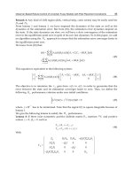
Figures 1 and 2 respectively show the behaviour of error
1
()et and
2
()et with and without
the
H
∞
approach and also the behaviour obtained using only lemma 1. We clearly see that
the estimation error converges faster in the first case (with
H
∞
approach and pole
placements) than in the second one (with pole placements only) as well as in the third case
(without
H
∞
approach and pole placements). At last but not least, Figure 3 and 4 show
respectively the behaviour of the state variables with and without the
H
∞
approach whereas
Figure 5
shows the evolution of the control signal. From Figures 3 and 4, we still have the
same conclusion about the convergence of the estimation errors.

0 0.2 0.4 0.6 0.8 1 1.2 1.4 1.6 1.8 2
-0.2
-0.15
-0.1
-0.05
0
0.05
Error e(1)
Time







Fig. 1. Behaviour of error
1
()et.
With the
H
∞
approach
Without the
H
∞

approach
Using lemma
1

Observer-Based Robust Control of Uncertain Fuzzy Models with Pole Placement Constraints

55
0 0.2 0.4 0.6 0.8 1 1.2 1.4 1.6 1.8 2
-0.4
-0.2
0
0.2
0.4
0.6
0.8
1
Error e(2)
Time

Fig. 2. Behaviour of error
2
()et
.
0.2 0.4 0.6 0.8 1 1.2 1.4 1.6
-0.2
-0.15
-0.1
-0.05
0
x(1) and estimed x(1)

0.1 0.2 0.3 0.4 0.5 0.6 0.7 0.8 0.9 1
-0.8
-0.6
-0.4
-0.2
0
0.2
x(2) and estimed x(2)
Time

Fig. 3. Behaviour of the state vector and its estimation with the
H
∞
approach.

2
()
x
t

2
ˆ
()
x
t
With the
H
∞
approach
Without the

H
∞
approach
Using lemma
1

1
()
x
t

1
ˆ
()
x
t

Recent Advances in Robust Control – Novel Approaches and Design Methods

56
0.2 0.4 0.6 0.8 1 1.2 1.4 1.6 1.8
-0.2
-0.15
-0.1
-0.05
0
x(1) and estimed x(1)
0.2 0.4 0.6 0.8 1 1.2 1.4 1.6 1.8
-0.4
-0.3

-0.2
-0.1
0
0.1
x(2) and estimed x(2)
Time

Fig. 4. Behaviour of the state and its estimation without the
H
∞
approach.
0.5 1 1.5 2 2.5
-0.05
0
0.05
0.1
0.15
0.2
0.25
0.3
0.35
Control signal u(t)
Time

Fig. 5. Control signal evolution
u(t).

1
()
x

t

1
ˆ
()
x
t

2
()
x
t

2
ˆ
()
x
t

Observer-Based Robust Control of Uncertain Fuzzy Models with Pole Placement Constraints

57
5. Conclusion
In this chapter, we have developed robust pole placement constraints for continuous T-S
fuzzy systems with unavailable state variables and with parametric structured uncertainties.
The proposed approach has extended existing methods based on uncertain T-S fuzzy
models. The proposed LMI constraints can globally asymptotically stabilize the closed-loop
T-S fuzzy system subject to parametric uncertainties with the desired control performances.
Because of uncertainties, the separation property is not applicable. To overcome this
problem, we have proposed, for the design of the observer and the controller, a two-step

procedure with two pole placements constraints and the minimization of a
H
∞
performance
criterion in order to guarantee that the estimation error converges faster to zero. Simulation
results have verified and confirmed the effectiveness of our approach in controlling
nonlinear systems with parametric uncertainties.
6. References
Chadli, M. & El Hajjaji, A. (2006). Comment on observer-based robust fuzzy control of
nonlinear systems with parametric uncertainties.
Fuzzy Sets and Systems, Vol. 157,
N°9 (2006), pp. 1276-1281
Boyd, S.; El Ghaoui, L. & Feron, E. & Balkrishnan, V. (1994)
. Linear Matrix Inequalities in
System and Control Theory
, Society for Industrial and Applied Mathematics, SIAM,
Philadelphia, USA
Chilali, M. & Gahinet, P. (1996).
H
∞
Design with Pole Placement Constraints: An LMI
Approach.
IEEE Transactions on Automatic Control, Vol. 41, N°3 (March 1996), pp.
358-367
Chilali, M.; Gahinet, P. & Apkarian, P. (1999). Robust Pole Placement in LMI Regions.
IEEE
Transactions on Automatic Control
, Vol. 44, N°12 (December 1999), pp. 2257-2270
El Messoussi, W.; Pagès, O. & El Hajjaji, A. (2005). Robust Pole Placement for Fuzzy Models
with Parametric Uncertainties: An LMI Approach,

Proceedings of the 4th Eusflat and
11
th
LFA Congress, pp. 810-815, Barcelona, Spain, September, 2005
El Messoussi, W.; Pagès, O. & El Hajjaji, A. (2006).Observer-Based Robust Control of
Uncertain Fuzzy Dynamic Systems with Pole Placement Constraints: An LMI
Approach,
Proceedings of the IEEE American Control conference, pp. 2203-2208,
Minneapolis, USA, June, 2006
Farinwata, S.; Filev, D. & Langari, R. (2000).
Fuzzy Control Synthesis and Analysis, John Wiley
& Sons, Ltd, pp. 267-282
Han, Z.X.; Feng, G. & Walcott, B.L. & Zhang, Y.M. (2000) .
H
∞
Controller Design of Fuzzy
Dynamic Systems with Pole Placement Constraints,
Proceedings of the IEEE American
Control Conference
, pp. 1939-1943, Chicago, USA, June, 2000
Hong, S. K. & Nam, Y. (2003). Stable Fuzzy Control System Design with Pole Placement
constraint: An LMI Approach.
Computers in Industry, Vol. 51, N°1 (May 2003), pp. 1-
11
Kang, G.; Lee, W. & Sugeno, M. (1998). Design of TSK Fuzzy Controller Based on TSK
Fuzzy Model Using Pole Placement,
Proceedings of the IEEE World Congress on
Computational Intelligence
, pp. 246 – 251, Vol. 1, N°12, Anchorage, Alaska, USA,
May, 1998

Recent Advances in Robust Control – Novel Approaches and Design Methods

58
Lauber J. (2003). Moteur à allumage commandé avec EGR: modélisation et commande non linéaires,
Ph. D. Thesis of the University of Valenciennes and Hainault-Cambresis, France,
December 2003, pp. 87-88
Lee, H.J.; Park, J.B. & Chen, G. (2001). Robust Fuzzy Control of Nonlinear Systems with
Parametric Uncertainties
. IEEE Transactions on Fuzzy Systems, Vol. 9, N°2, (April
2001), pp. 369-379
Lo, J. C. & Lin, M. L. (2004). Observer-Based Robust
H
∞
Control for Fuzzy Systems Using
Two-Step Procedure.
IEEE Transactions on Fuzzy Systems, Vol. 12, N°3, (June 2004),
pp. 350-359
Ma, X. J., Sun Z. Q. & He, Y. Y. (1998). Analysis and Design of Fuzzy Controller and Fuzzy
Observer.
IEEE Transactions on Fuzzy Systems, Vol. 6, N°1, (February 1998), pp. 41-
51
Shi, G., Zou Y. & Yang, C. (1992). An algebraic approach to robust
H
∞
control via state
feedback.
System Control Letters, Vol. 18, N°5 (1992), pp. 365-370
Tanaka, K.; Ikeda, T. & Wang, H. O. (1998). Fuzzy Regulators and Fuzzy Observers: Relaxed
Stability Conditions and LMI-Based Design

. IEEE Transactions on Fuzzy Systems,
Vol. 6, N°2, (May 1998), pp. 250-265
Tong, S. & Li, H. H. (1995). Observer-based robust fuzzy control of nonlinear systems with
parametric uncertainties.
Fuzzy Sets and Systems, Vol. 131, N°2, (October 2002), pp.
165-184
Wang, S. G.; Shieh, L. S. & Sunkel, J. W. (1995). Robust optimal pole-placement in a vertical
strip and disturbance rejection in Structured Uncertain Systems
. International
Journal of System Science
, Vol. 26, (1995), pp. 1839-1853
Wang, S. G.; Shieh, L. S. & Sunkel, J. W. (1998). Observer-Based controller for Robust Pole
Clustering in a vertical strip and disturbance rejection.
International Journal of
Robust and Nonlinear Control
, Vol. 8, N°5, (1998), pp. 1073-1084
Wang, S. G.; Yeh, Y. & Roschke, P. N. (2001). Robust Control for Structural Systems with
Parametric and Unstructured Uncertainties,
Proceedings of the American Control
Conference
, pp. 1109-1114, Arlington, USA, June 2001
Xiaodong, L. & Qingling, Z. (2003). New approaches to
H
∞
controller designs based on
fuzzy observers for T-S fuzzy systems via LMI.
Automatica, Vol. 39, N° 9,
(September 2003), pp. 1571-1582
Yoneyama, J; Nishikawa, M.; Katayama, H. & Ichikawa, A. (2000). Output stabilization of
Takagi-Sugeno fuzzy systems.

Fuzzy Sets and Systems, Vol. 111, N°2, April 2000, pp.
253-266
4
Robust Control Using LMI Transformation and
Neural-Based Identification for Regulating
Singularly-Perturbed Reduced Order
Eigenvalue-Preserved Dynamic Systems
Anas N. Al-Rabadi
Computer Engineering Department, The University of Jordan, Amman
Jordan
1. Introduction
In control engineering, robust control is an area that explicitly deals with uncertainty in its
approach to the design of the system controller [7,10,24]. The methods of robust control are
designed to operate properly as long as disturbances or uncertain parameters are within a
compact set, where robust methods aim to accomplish robust performance and/or stability
in the presence of bounded modeling errors. A robust control policy is static in contrast to
the adaptive (dynamic) control policy where, rather than adapting to measurements of
variations, the system controller is designed to function assuming that certain variables will
be unknown but, for example, bounded. An early example of a robust control method is the
high-gain feedback control where the effect of any parameter variations will be negligible
with using sufficiently high gain.
The overall goal of a control system is to cause the output variable of a dynamic process to
follow a desired reference variable accurately. This complex objective can be achieved based
on a number of steps. A major one is to develop a mathematical description, called
dynamical model, of the process to be controlled [7,10,24]. This dynamical model is usually
accomplished using a set of differential equations that describe the dynamic behavior of the
system, which can be further represented in state-space using system matrices or in
transform-space using transfer functions [7,10,24].
In system modeling, sometimes it is required to identify some of the system parameters.
This objective maybe achieved by the use of artificial neural networks (ANN), which are

considered as the new generation of information processing networks [5,15,17,28,29].
Artificial neural systems can be defined as physical cellular systems which have the
capability of acquiring, storing and utilizing experiential knowledge [15,29], where an ANN
consists of an interconnected group of basic processing elements called neurons that
perform summing operations and nonlinear function computations. Neurons are usually
organized in layers and forward connections, and computations are performed in a parallel
mode at all nodes and connections. Each connection is expressed by a numerical value
called the weight, where the conducted learning process of a neuron corresponds to the
changing of its corresponding weights.

Recent Advances in Robust Control – Novel Approaches and Design Methods

60
When dealing with system modeling and control analysis, there exist equations and
inequalities that require optimized solutions. An important expression which is used in
robust control is called linear matrix inequality (LMI) which is used to express specific
convex optimization problems for which there exist powerful numerical solvers [1,2,6].
The important LMI optimization technique was started by the Lyapunov theory showing
that the differential equation
() ()xt Axt
=

is stable if and only if there exists a positive
definite matrix [P] such that
0
T
AP PA
+
<
[6]. The requirement of { 0P > ,

0
T
AP PA+<
} is
known as the Lyapunov inequality on [P] which is a special case of an LMI. By picking any
0
T
QQ=> and then solving the linear equation
T
AP PA Q
+
=− for the matrix [P], it is
guaranteed to be positive-definite if the given system is stable. The linear matrix inequalities
that arise in system and control theory can be generally formulated as convex optimization
problems that are amenable to computer solutions and can be solved using algorithms such
as the ellipsoid algorithm [6].
In practical control design problems, the first step is to obtain a proper mathematical model
in order to examine the behavior of the system for the purpose of designing an appropriate
controller [1,2,3,4,5,7,8,9,10,11,12,13,14,16,17,19,20,21,22,24,25,26,27]. Sometimes, this
mathematical description involves a certain small parameter (i.e., perturbation). Neglecting
this small parameter results in simplifying the order of the designed controller by reducing
the order of the corresponding system [1,3,4,5,8,9,11,12,13,14,17,19,20,21,22,25,26]. A reduced
model can be obtained by neglecting the fast dynamics (i.e., non-dominant eigenvalues) of
the system and focusing on the slow dynamics (i.e., dominant eigenvalues). This
simplification and reduction of system modeling leads to controller cost minimization
[7,10,13]. An example is the modern integrated circuits (ICs), where increasing package
density forces developers to include side effects. Knowing that these ICs are often modeled
by complex RLC-based circuits and systems, this would be very demanding
computationally due to the detailed modeling of the original system [16]. In control system,
due to the fact that feedback controllers don't usually consider all of the dynamics of the

functioning system, model reduction is an important issue [4,5,17].
The main results in this research include the introduction of a new layered method of
intelligent control, that can be used to robustly control the required system dynamics, where
the new control hierarchy uses recurrent supervised neural network to identify certain
parameters of the transformed system matrix [

A
], and the corresponding LMI is used to
determine the permutation matrix [P] so that a complete system transformation {[

B
], [

C
],
[

D
]} is performed. The transformed model is then reduced using the method of singular
perturbation and various feedback control schemes are applied to enhance the
corresponding system performance, where it is shown that the new hierarchical control
method simplifies the model of the dynamical systems and therefore uses simpler
controllers that produce the needed system response for specific performance
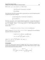
enhancements. Figure 1 illustrates the layout of the utilized new control method. Layer 1
shows the continuous modeling of the dynamical system. Layer 2 shows the discrete system
model. Layer 3 illustrates the neural network identification step. Layer 4 presents the
undiscretization of the transformed system model. Layer 5 includes the steps for model
order reduction with and without using LMI. Finally, Layer 6 presents various feedback
control methods that are used in this research.
Robust Control Using LMI Transformation and Neural-Based Identification for

Regulating Singularly-Perturbed Reduced Order Eigenvalue-Preserved Dynamic Systems

61
Continuous Dynamic System: {[A], [B], [C], [D]}
System Discretization
System Undiscretization (Continuous form)
LMI-Based Permutation
Matrix [P]

Model Order Reduction

Output Feedback
(LQR Optimal
Control)

PID

State Feedback (
LQR
Optimal Control)
State Feedback
(Pole Placement)
Closed-Loop Feedback Control
Neural-Based System
Transformation: {[
A
ˆ
],[

B

ˆ
]}
Neural-Based State
Transformation: [
A
~
]

Complete System
Transformation: {[
B
~
],[
C
~
],[
D
~
]}

State
Feedback
Control


Fig. 1. The newly utilized hierarchical control method.
While similar hierarchical method of ANN-based identification and LMI-based
transformation has been previously utilized within several applications such as for the
reduced-order electronic Buck switching-mode power converter [1] and for the reduced-
order quantum computation systems [2] with relatively simple state feedback controller

implementations, the presented method in this work further shows the successful wide
applicability of the introduced intelligent control technique for dynamical systems using
various spectrum of control methods such as (a) PID-based control, (b) state feedback
control using (1) pole placement-based control and (2) linear quadratic regulator (LQR)
optimal control, and (c) output feedback control.
Section 2 presents background on recurrent supervised neural networks, linear matrix
inequality, system model transformation using neural identification, and model order
reduction. Section 3 presents a detailed illustration of the recurrent neural network
identification with the LMI optimization techniques for system model order reduction. A
practical implementation of the neural network identification and the associated
comparative results with and without the use of LMI optimization to the dynamical system
model order reduction is presented in Section 4. Section 5 presents the application of the
feedback control on the reduced model using PID control, state feedback control using pole
assignment, state feedback control using LQR optimal control, and output feedback control.
Conclusions and future work are presented in Section 6.

Recent Advances in Robust Control – Novel Approaches and Design Methods

62
2. Background
The following sub-sections provide an important background on the artificial supervised
recurrent neural networks, system transformation without using LMI, state transformation
using LMI, and model order reduction, which can be used for the robust control of dynamic
systems, and will be used in the later Sections 3-5.
2.1 Artificial recurrent supervised neural networks
The ANN is an emulation of the biological neural system [15,29]. The basic model of the
neuron is established emulating the functionality of a biological neuron which is the basic
signaling unit of the nervous system. The internal process of a neuron maybe
mathematically modeled as shown in Figure 2 [15,29].

Fig. 2. A mathematical model of the artificial neuron.
As seen in Figure 2, the internal activity of the neuron is produced as:

1
p
kk
jj
j
vwx
=
=
∑
(1)
In supervised learning, it is assumed that at each instant of time when the input is applied, the
desired response of the system is available [15,29]. The difference between the actual and the
desired response represents an error measure which is used to correct the network parameters
externally. Since the adjustable weights are initially assumed, the error measure may be used
to adapt the network's weight matrix [W]. A set of input and output patterns, called a training
set, is required for this learning mode, where the usually used training algorithm identifies
directions of the negative error gradient and reduces the error accordingly [15,29].
The supervised recurrent neural network used for the identification in this research is based
on an approximation of the method of steepest descent [15,28,29]. The network tries to
match the output of certain neurons to the desired values of the system output at a specific
instant of time. Consider a network consisting of a total of
N neurons with M external input
connections, as shown in Figure 3, for a 2
nd
order system with two neurons and one external

input. The variable g(
k) denotes the (M x 1) external input vector which is applied to the
0k
w
1k
w
2k
w
∑


().
ϕ
k
y
1
x

2
x
p
x
Output
Activation
Function
Summing
Junction
Synaptic
Weights
Input

Signals
k
v
Threshold
k
θ

kp
w
0
x
Robust Control Using LMI Transformation and Neural-Based Identification for
Regulating Singularly-Perturbed Reduced Order Eigenvalue-Preserved Dynamic Systems

63
network at discrete time k, the variable y(k + 1) denotes the corresponding (N x 1) vector of
individual neuron outputs produced one step later at time (
k + 1), and the input vector g(k)
and one-step delayed output vector y(
k) are concatenated to form the ((M + N) x 1) vector
u(
k) whose i
th
element is denoted by u
i
(k). For Λ denotes the set of indices i for which g
i
(k) is
an external input, and
β denotes the set of indices i for which u

i
(k) is the output of a
neuron (which is
y
i
(k)), the following equation is provided:
if
()
()
if
()
i
i
i
g i Λ
k,
k =
u
y i
k,
β
∈
⎧
⎪
⎨
∈
⎪
⎩

Fig. 3. The utilized 2
nd
order recurrent neural network architecture, where the identified
matrices are given by {
11 12 11
21 22 21
,
dd
AA B
AB
AA B
⎡
⎤⎡⎤
==
⎢
⎥⎢⎥
⎣
⎦⎣⎦


} and that [ ] [ ]W
⎡
⎤
=
⎣
⎦


dd

AB.
The (
N x (M + N)) recurrent weight matrix of the network is represented by the variable [W].
The net internal activity of neuron j at time k is given by:


() = () ()
jjii
i Λ
vk w kuk
β
∈∪
∑


where Λ ∪
ß
is the union of sets Λ and
ß
. At the next time step (k + 1), the output of the
neuron j is computed by passing v
j
(k) through the nonlinearity
(.)
ϕ
, thus obtaining:

(1) = (())
jj
y

kvk
ϕ
+

The derivation of the recurrent algorithm can be started by using d
j
(k) to denote the desired
(target) response of neuron j at time k, and ς(k) to denote the set of neurons that are chosen
to provide externally reachable outputs. A time-varying (N x 1) error vector e(k) is defined
whose j
th
element is given by the following relationship:
Z
-1

g
1
:
A
11

A
12

A
21

A
22

B
11

B
21

)1(
~
1
+
kx
System
external input
System
d
y
namics
System state:
internal input
Neuron
delay
Z
-1

Outputs

)(
~
ky

)1(
~
2
+
kx
)(
~
1
kx
)(
~
2
kx









Recent Advances in Robust Control – Novel Approaches and Design Methods

64
() - (), if ()
() =
0, otherwise
jj
j

dk
y
k
j
k
ek
ς
∈
⎧
⎪
⎨
⎪
⎩

The objective is to minimize the cost function E
total
which is obtained by:
total
= ( )
k
EEk
∑
, where

2
1
() = ()
2
j
j

Ek e k
ς
∈
∑

To accomplish this objective, the method of steepest descent which requires knowledge of
the gradient matrix is used:

total
total
()
= = = ( )
kk
E
Ek
EEk
∂
∂
∇∇
∂
∂
∑∑
WW
W
W

where
()Ek∇
W
is the gradient of E(k) with respect to the weight matrix [W]. In order to train

the recurrent network in real time, the instantaneous estimate of the gradient is used
(
)
()Ek∇
W
. For the case of a particular weight
m
w
A
(k), the incremental change
m
wΔ
A
(k)
made at k is defined as
()
() = -
()
m
m
Ek
wk
wk
η
∂
Δ
∂
A
A
where η is the learning-rate parameter.

Therefore:

()
()
()
= ( ) = - ( )
() () ()

j
i
jj
mm m
jj
ek
y
k
Ek
ek ek
wk wk wk
ςς
∈∈
∂
∂
∂
∂∂ ∂
∑∑
AA A


To determine the partial derivative ( )/ ( )

jm
y
kwk
∂
∂
A
, the network dynamics are derived. This
derivation is obtained by using the chain rule which provides the following equation:
( + 1) ( +1) ( ) ( )
= = ( ( ))
() () () ()
jjj j
j
mjm m
y
k
y
kvk vk
vk
wk vk wk wk
ϕ
∂∂∂ ∂
∂∂∂ ∂
AAA

, where
(())
(()) =
()
j

j
j
vk
vk
vk
ϕ
ϕ
∂
∂

.
Differentiating the net internal activity of neuron j with respect to
m
w
A
(k) yields:

() ()
(()())
()
= = () + ()
()
() () ()
j ji
ji i
i
ji i
m
mmm
i Λ i Λ

vk w k
wkuk
uk
wk uk
wk
wk wk wk
ββ
∈∪ ∈∪
∂∂
∂
⎡
⎤
∂
⎢
⎥
∂
∂∂∂
⎢
⎥
⎣
⎦
∑∑
A
AAA

where
(
)
()/ ()
ji m

wk w k∂∂
A
equals "1" only when j = m and i = A , and "0" otherwise. Thus:

()
= ( )
()
j
i
mj
ji
mm
i Λ
vk
(k)
u
wk u(k)
δ
wk w(k)
β
∈∪
∂
∂
+
∂∂
∑
A
AA

where

m
j
δ
is a Kronecker delta equals to "1" when j = m and "0" otherwise, and:
0, if
()
=
()
, if
()
()
i
i
m
m
i
Λ
uk
yk
i
wk
wk
β
∈
⎧
∂
⎪
∂
⎨
∈

∂
⎪
∂
⎩
A
A

Robust Control Using LMI Transformation and Neural-Based Identification for
Regulating Singularly-Perturbed Reduced Order Eigenvalue-Preserved Dynamic Systems

65
Having those equations provides that:

(+1)
()
= ( ( )) ( ) ( )
() ()

j
i
m
jji
mm
i
yk
yk
vk w k uk
wk wk
β
ϕ

δ
∈
⎡
⎤
∂
∂
+
⎢
⎥
∂∂
⎢
⎥
⎣
⎦
∑
A
A
AA


The initial state of the network at time (k = 0) is assumed to be zero as follows:
(0)
= 0
(0)
i
m
y
w
∂
∂

A
, for {j
∈
ß
, m
∈
ß
, A
∈
Λ
β
∪ }.
The dynamical system is described by the following triply-indexed set of variables (
j
m
π
A
):
()
() =
()
j
j
m
m
y
k
k
wk
π

∂
∂
A
A

For every time step k and all appropriate j, m and
A , system dynamics are controlled by:

(+1) = ( ()) () () ()
j
i
mj
j
ji m
m
i
kkwkkuk
v
β
πϕ π
δ
∈
⎡
⎤
+
⎢
⎥
⎢
⎥
⎣

⎦
∑
AA
A

, with (0) = 0
j
m
π
A
.
The values of
()
j
m
k
π
A
and the error signal e
j
(k) are used to compute the corresponding
weight changes:


() = () ()
j
m
j
m
j

kekk
w
ς
η
π
∈
Δ
∑
A
A
(2)
Using the weight changes, the updated weight
m
w
A
(k + 1) is calculated as follows:

(+1) = () + ()
mmm
wk wk wk
Δ
AAA
(3)
Repeating this computation procedure provides the minimization of the cost function and
thus the objective is achieved. With the many advantages that the neural network has, it is
used for the important step of parameter identification in model transformation for the
purpose of model order reduction as will be shown in the following section.
2.2 Model transformation and linear matrix inequality
In this section, the detailed illustration of system transformation using LMI optimization
will be presented. Consider the dynamical system:

() () ()xt Axt But=+

(4)

() () ()
y
tCxtDut
=
+ (5)
The state space system representation of Equations (4) - (5) may be described by the block
diagram shown in Figure 4.

Recent Advances in Robust Control – Novel Approaches and Design Methods

66

Fig. 4. Block diagram for the state-space system representation.
In order to determine the transformed [
A] matrix, which is [

A
], the discrete zero input
response is obtained. This is achieved by providing the system with some initial state values
and setting the system input to zero (u(k) = 0). Hence, the discrete system of Equations
(4) - (5), with the initial condition
0
(0)xx
=

, becomes:

(1) ()
d
xk Axk
+
= (6)

() ()
y
kxk
=
(7)
We need x(k) as an ANN target to train the network to obtain the needed parameters in
[

d
A ] such that the system output will be the same for [A
d
] and [

d
A ]. Hence, simulating this
system provides the state response corresponding to their initial values with only the [
A
d
]
matrix is being used. Once the input-output data is obtained, transforming the [
A
d

] matrix is
achieved using the ANN training, as will be explained in Section 3. The identified
transformed [

d
A ] matrix is then converted back to the continuous form which in general
(with all real eigenvalues) takes the following form:

0
rc
o
AA
A
A
⎡
⎤
=
⎢
⎥
⎣
⎦

→
112 1
22
0
0
00
n
n

n
AA
A
A
λ
λ
λ
⎡
⎤
⎢
⎥
⎢
⎥
=
⎢
⎥
⎢
⎥
⎢
⎥
⎣
⎦

"

"

#%#
"
(8)

where λ
i
represents the system eigenvalues. This is an upper triangular matrix that
preserves the eigenvalues by (1) placing the original eigenvalues on the diagonal and (2)
finding the elements

ij
A
in the upper triangular. This upper triangular matrix form is used
to produce the same eigenvalues for the purpose of eliminating the fast dynamics and
sustaining the slow dynamics eigenvalues through model order reduction as will be shown
in later sections.
Having the [
A] and [

A
] matrices, the permutation [P] matrix is determined using the LMI
optimization technique, as will be illustrated in later sections. The complete system
transformation can be achieved as follows where, assuming that
1
xPx
−
=

, the system of
Equations (4) - (5) can be re-written as:
() () ()Px t APx t Bu t=+


,

() () ()
y
tCPxtDut=+

, where
() ()
y
tyt=

.
B
∫

C
D
A
+
+
+
y(t)
u(t)
)(tx


)(tx
+
Robust Control Using LMI Transformation and Neural-Based Identification for
Regulating Singularly-Perturbed Reduced Order Eigenvalue-Preserved Dynamic Systems

67

Pre-multiplying the first equation above by [P
-1
], one obtains:
11 1
() () ()PPxt PAPxt PBut
−
−−
=+


, () () ()
y
tCPxtDut
=
+


which yields the following transformed model:

() () ()
xt Axt But=+



(9)

() () ()
y
tCxtDut=+




(10)
where the transformed system matrices are given by:

1
A
PAP
−
=

(11)

1
BPB
−
=

(12)

CCP
=

(13)

DD
=

(14)
Transforming the system matrix [

A] into the form shown in Equation (8) can be achieved
based on the following definition [18].
Definition. A matrix
n
AM
∈
is called reducible if either:
a.
n = 1 and A = 0; or
b. n ≥ 2, there is a permutation matrix
n
PM
∈
, and there is some integer r with
11
rn≤≤− such that:

1
XY
PAP
Z
−
⎡
⎤
=
⎢
⎥
⎣
⎦
0

(15)
where
,rr
XM∈ ,
,nrnr
ZM
−
−
∈
,
,rn r
YM
−
∈
, and 0
,nrr
M
−
∈
is a zero matrix.
The attractive features of the permutation matrix [
P] such as being (1) orthogonal and (2)
invertible have made this transformation easy to carry out. However, the permutation
matrix structure narrows the applicability of this method to a limited category of
applications. A form of a similarity transformation can be used to correct this problem for
{
:
nn nn
fR R
××

→
} where
f
is a linear operator defined by
1
()
f
APAP
−
=
[18]. Hence, based
on [
A] and [

A ], the corresponding LMI is used to obtain the transformation matrix [P], and
thus the optimization problem will be casted as follows:

1
min
o
P
PP SubjecttoPAPA
ε
−
−
−<

(16)
which can be written in an LMI equivalent form as:

21
1
1
min ( ) 0
()
0
()
o
T
S
o
T
SPP
trace S Subject to
PP I
IPAPA
PAP A I
ε
−
−
−
⎡⎤
>
⎢⎥
−
⎢⎥
⎣⎦
⎡⎤
−
>

⎢⎥
−
⎢⎥
⎣⎦


(17)

Recent Advances in Robust Control – Novel Approaches and Design Methods

68
where S is a symmetric slack matrix [6].
2.3 System transformation using neural identification
A different transformation can be performed based on the use of the recurrent ANN while
preserving the eigenvalues to be a subset of the original system. To achieve this goal, the
upper triangular block structure produced by the permutation matrix, as shown in Equation
(15), is used. However, based on the implementation of the ANN, finding the permutation
matrix [
P] does not have to be performed, but instead [X] and [Z] in Equation (15) will
contain the system eigenvalues and [
Y] in Equation (15) will be estimated directly using the
corresponding ANN techniques. Hence, the transformation is obtained and the reduction is
then achieved. Therefore, another way to obtain a transformed model that preserves the
eigenvalues of the reduced model as a subset of the original system is by using ANN
training without the LMI optimization technique. This may be achieved based on the
assumption that the states are reachable and measurable. Hence, the recurrent ANN can
identify the [
d
ˆ
A] and [

d
ˆ
B ] matrices for a given input signal as illustrated in Figure 3. The
ANN identification would lead to the following [
d
ˆ
A] and [
d
ˆ
B ] transformations which (in
the case of all real eigenvalues) construct the weight matrix [
W] as follows:
1
112 1
2
22
ˆ
ˆˆ
ˆ
ˆ
0
ˆˆ
ˆˆ
[ ] [ ] ,
0
ˆ
00
n
n
dd

n
n
b
AA
b
A
WAB A B
b
λ
λ
λ
⎡
⎤
⎡⎤
⎢
⎥
⎢⎥
⎢
⎥
⎢⎥
⎡⎤
=→= =
⎢
⎥
⎢⎥
⎣⎦
⎢
⎥
⎢⎥
⎢

⎥
⎢⎥
⎣⎦
⎣
⎦
"
"
#
#%#
"

where the eigenvalues are selected as a subset of the original system eigenvalues.
2.4 Model order reduction
Linear time-invariant (LTI) models of many physical systems have fast and slow dynamics,
which may be referred to as singularly perturbed systems [19]. Neglecting the fast dynamics
of a singularly perturbed system provides a reduced (i.e., slow) model. This gives the
advantage of designing simpler lower-dimensionality reduced-order controllers that are
based on the reduced-model information.
To show the formulation of a reduced order system model, consider the singularly
perturbed system [9]:

11 12 1 0
() () () () , 0xt A xt A t But x( ) x
ξ
=
++ =

(18)

21 22 2 0

() () () () , (0tAxtA tBut )
ε
ξξξξ
=
++ =

(19)

12
y
() () ()tCxtCt
ξ
=
+ (20)
where
1

m
x ∈ℜ and
2
m
ξ
∈
ℜ are the slow and fast state variables, respectively,
1

n
u∈ℜ and
2
n

y ∈ℜ are the input and output vectors, respectively, {[]
ii
A , [
i
B ], [
i
C ]} are constant
matrices of appropriate dimensions with
{1, 2}i ∈
, and
ε
is a small positive constant. The
singularly perturbed system in Equations (18)-(20) is simplified by setting 0
ε
=
[3,14,27]. In
Robust Control Using LMI Transformation and Neural-Based Identification for
Regulating Singularly-Perturbed Reduced Order Eigenvalue-Preserved Dynamic Systems

69
doing so, we are neglecting the fast dynamics of the system and assuming that the state
variables
ξ
have reached the quasi-steady state. Hence, setting 0
ε
=
in Equation (19), with
the assumption that [
22
A

] is nonsingular, produces:

11
22 21 22 1
() () ()
r
tAAxtABut
ξ
−
−
=− −
(21)
where the index r denotes the remained or reduced model. Substituting Equation (21) in
Equations (18)-(20) yields the following reduced order model:

() () ()
rrrr
xt Axt But
=
+

(22)

() () ()
rr r
y
tCxtDut=+ (23)
where {
1
11 12 22 21r

AA AAA
−
=− ,
1
112222r
BBAAB
−
=− ,
1
1 2 22 21r
CCCAA
−
=− ,
1
2222r
DCAB
−
=− }.
3. Neural network identification with lmi optimization for the system model
order reduction
In this work, it is our objective to search for a similarity transformation that can be used to
decouple a pre-selected eigenvalue set from the system matrix [
A]. To achieve this objective,
training the neural network to identify the transformed discrete system matrix [

d
A ] is
performed [1,2,15,29]. For the system of Equations (18)-(20), the discrete model of the
dynamical system is obtained as:

(1) () ()
dd
xk Axk Buk
+
=+
(24)

() () ()
dd
y
kCxkDuk
=
+
(25)
The identified discrete model can be written in a detailed form (as was shown in Figure 3) as
follows:

11112111
2 21222 21
(1) ()
()
(1) ()
xk A A xk B
uk
xk A A xk B
+
⎡⎤⎡ ⎤⎡⎤⎡⎤
=+
⎢⎥⎢ ⎥⎢⎥⎢⎥
+

⎣
⎦⎣ ⎦⎣ ⎦⎣ ⎦


(26)

1
2
()
()
()
xk
yk
xk
⎡
⎤
=
⎢
⎥
⎣
⎦



(27)
where k is the time index, and the detailed matrix elements of Equations (26)-(27) were
shown in Figure 3 in the previous section.
The recurrent ANN presented in Section 2.1 can be summarized by defining Λ as the set of
indices i for which
()

i
gkis an external input, defining ß as the set of indices i for which
()
i
ykis an internal input or a neuron output, and defining ()
i
ukas the combination of the
internal and external inputs for which
iß
∈
∪ Λ. Using this setting, training the ANN
depends on the internal activity of each neuron which is given by:

() () ()
jjii
i Λ
vk w kuk
β
∈∪
=
∑
(28)

Recent Advances in Robust Control – Novel Approaches and Design Methods

70
where w
ji
is the weight representing an element in the system matrix or input matrix for
jß∈ and iß∈∪Λ such that [ ] [ ]W

⎡
⎤
=
⎣
⎦


dd
AB. At the next time step (k +1), the output
(internal input) of the neuron j is computed by passing the activity through the nonlinearity
φ(.) as follows:

(1)(())
jj
xk vk
ϕ
+
=
(29)

With these equations, based on an approximation of the method of steepest descent, the
ANN identifies the system matrix [
A
d
] as illustrated in Equation (6) for the zero input
response. That is, an error can be obtained by matching a true state output with a neuron
output as follows:
() () ()
jjj
ek xk xk

=
−


Now, the objective is to minimize the cost function given by:
total
()
k
EEk=
∑
and
2
1
2
() ()
j
j
Ek e k
ς
∈
=
∑

where
ς
denotes the set of indices j for the output of the neuron structure. This cost
function is minimized by estimating the instantaneous gradient of E(k) with respect to the
weight matrix [
W] and then updating [W] in the negative direction of this gradient [15,29].
In steps, this may be proceeded as follows:

-
Initialize the weights [W] by a set of uniformly distributed random numbers. Starting at
the instant (k = 0), use Equations (28) - (29) to compute the output values of the N
neurons (where
Nß
=
).
-
For every time step k and all ,jß∈ mß
∈
and
ß
∈
∪A Λ, compute the dynamics of the
system which are governed by the triply-indexed set of variables:
(1)(()) ()() ()
j
i
jjimmj
m
iß
kvkwkkuk
πϕ πδ
∈
⎡
⎤
+= +
⎢
⎥
⎢

⎥
⎣
⎦
∑
AA
A


with initial conditions
(0) 0
j
m
π
=
A
and
m
j
δ
is given by
(
)
() ()
ji m
wk w k∂∂
A
, which is equal
to "1" only when {j = m, i
=
A } and otherwise it is "0". Notice that, for the special case of

a sigmoidal nonlinearity in the form of a logistic function, the derivative
()
ϕ
⋅

is given
by ( ( )) ( 1)[1 ( 1)]
jj j
vk y k yk
ϕ
=+−+

.
-
Compute the weight changes corresponding to the error signal and system dynamics:

() () ()
j
mj
m
j
wk ek k
ς
ηπ
∈
Δ=
∑
A
A
(30)

-
Update the weights in accordance with:

(1) () ()
mmm
wk wk wk
+
=+Δ
AAA
(31)
-
Repeat the computation until the desired identification is achieved.
Robust Control Using LMI Transformation and Neural-Based Identification for
Regulating Singularly-Perturbed Reduced Order Eigenvalue-Preserved Dynamic Systems

71
As illustrated in Equations (6) - (7), for the purpose of estimating only the transformed
system matrix [

d
A
], the training is based on the zero input response. Once the training is
completed, the obtained weight matrix [
W] will be the discrete identified transformed
system matrix [

d
A ]. Transforming the identified system back to the continuous form yields
the desired continuous transformed system matrix [


A
]. Using the LMI optimization
technique, which was illustrated in Section 2.2, the permutation matrix [
P] is then determined.
Hence, a complete system transformation, as shown in Equations (9) - (10), will be achieved.
For the model order reduction, the system in Equations (9) - (10) can be written as:

() ()
()
0()
()
rrcrr
oo o
o
xt A A xt B
ut
Axt B
xt
⎡⎤
⎡⎤⎡⎤⎡⎤
=+
⎢⎥
⎢⎥⎢⎥⎢⎥
⎢⎥
⎣⎦⎣⎦⎣⎦
⎣
⎦






(32)

[]
() ()
()
() ()
rrr
ro
ooo
yt xt D
CC ut
yt xt D
⎡⎤ ⎡⎤⎡⎤
=+
⎢⎥ ⎢⎥⎢⎥
⎣
⎦⎣⎦⎣⎦


(33)
The following system transformation enables us to decouple the original system into
retained (r) and omitted (o) eigenvalues. The retained eigenvalues are the dominant
eigenvalues that produce the slow dynamics and the omitted eigenvalues are the non-
dominant eigenvalues that produce the fast dynamics. Equation (32) maybe written as:
() () () ()
rrrcor
xt Axt Axt But=++



and
() () ()
oooo
xt Axt But=+



The coupling term
()
co
Ax t

maybe compensated for by solving for ()
o
xt

in the second
equation above by setting
()
o
xt


to zero using the singular perturbation method (by
setting 0
ε
= ). By performing this, the following equation is obtained:

1

() ()
ooo
xt A But
−
=−

(34)
Using
()
o
xt

, we get the reduced order model given by:

1
() () [ ]()
rrr coor
xt Axt AA B But
−
=+− +


(35)

1
() () [ ]()
rr o o o
y
tCxt CABDut
−

=+− +

(36)
Hence, the overall reduced order model may be represented by:
( ) ( ) ( )
rorror
xt Axt But=+


(37)

() () ()
or r or
y
tCxtDut
=
+

(38)
where the details of the {[
or
A ], [
or
B ], [
or
C ], [
or
D ]} overall reduced matrices were shown in
Equations (35) - (36), respectively.
4. Examples for the dynamic system order reduction using neural

identification
The following subsections present the implementation of the new proposed method of
system modeling using supervised ANN, with and without using LMI, and using model

Recent Advances in Robust Control – Novel Approaches and Design Methods

72
order reduction, that can be directly utilized for the robust control of dynamic systems. The
presented simulations were tested on a PC platform with hardware specifications of Intel
Pentium 4 CPU 2.40 GHz, and 504 MB of RAM, and software specifications of MS Windows
XP 2002 OS and Matlab 6.5 simulator.
4.1 Model reduction using neural-based state transformation and lmi-based
complete system transformation
The following example illustrates the idea of dynamic system model order reduction using
LMI with comparison to the model order reduction without using LMI. Let us consider the
system of a high-performance tape transport which is illustrated in Figure 5. As seen in
Figure 5, the system is designed with a small capstan to pull the tape past the read/write
heads with the take-up reels turned by DC motors [10].


(a)

(b)
Fig. 5. The used tape drive system: (a) a front view of a typical tape drive mechanism, and
(b) a schematic control model.
Robust Control Using LMI Transformation and Neural-Based Identification for
Regulating Singularly-Perturbed Reduced Order Eigenvalue-Preserved Dynamic Systems

73
As can be shown, in static equilibrium, the tape tension equals the vacuum force (

o
TF= )
and the torque from the motor equals the torque on the capstan (
1to o
Ki rT
=
) where T
o
is the
tape tension at the read/write head at equilibrium, F is the constant force (i.e., tape tension
for vacuum column), K is the motor torque constant, i
o
is the equilibrium motor current, and
r
1
is the radius of the capstan take-up wheel.
The system variables are defined as deviations from this equilibrium, and the system
equations of motion are given as follows:
1
1111
t
d
JrTKi
dt
ω
βω
=+ −+
,
111
xr

ω
=


1e
di
LRiK e
dt
ω
+=
,
222
xr
ω
=


2
2222
0
d
JrT
dt
ω
βω
++=

13 1 13 1
()()TKx x Dx x=−+−


22 3 22 3
()()TKx x Dx x=−+−


111
xr
θ
= ,
222
xr
θ
= ,
12
3
2
xx
x
−
=

where
1,2
D is the damping in the tape-stretch motion, e is the applied input voltage (V), i is
the current into capstan motor, J
1
is the combined inertia of the wheel and take-up motor, J
2

is the inertia of the idler, K

1,2
is the spring constant in the tape-stretch motion, K
e
is the
electric constant of the motor, K
t
is the torque constant of the motor, L is the armature
inductance, R is the armature resistance, r
1
is the radius of the take-up wheel, r
2
is the radius
of the tape on the idler, T is the tape tension at the read/write head, x
3
is the position of the
tape at the head,
3
x

is the velocity of the tape at the head, β
1
is the viscous friction at take-
up wheel, β
2
is the viscous friction at the wheel, θ
1
is the angular displacement of the
capstan, θ
2
is the tachometer shaft angle, ω

1
is the speed of the drive wheel
1
θ

, and ω
2
is the
output speed measured by the tachometer output
2
θ

.
The state space form is derived from the system equations, where there is one input, which
is the applied voltage, three outputs which are (1) tape position at the head, (2) tape tension,
and (3) tape position at the wheel, and five states which are (1) tape position at the air
bearing, (2) drive wheel speed, (3) tape position at the wheel, (4) tachometer output speed,
and (5) capstan motor speed. The following sub-sections will present the simulation results
for the investigation of different system cases using transformations with and without
utilizing the LMI optimization technique.
4.1.1 System transformation using neural identification without utilizing linear matrix
inequality
This sub-section presents simulation results for system transformation using ANN-based
identification and without using LMI.
Case #1. Let us consider the following case of the tape transport:
02000 0
-1.1 -1.35 1.1 3.1 0.75 0
00050 0
() () ()
1.35 1.4 -2.4 -11.4 0 0

0 -0.03 0 0 -10 1
xt xt ut
⎡⎤⎡⎤
⎢⎥⎢⎥
⎢⎥⎢⎥
⎢⎥⎢⎥
=+
⎢⎥⎢⎥
⎢⎥⎢⎥
⎢⎥⎢⎥
⎣⎦⎣⎦

,