Mechatronic Servo System Control - M. Nakamura S. Goto and N. Kyura Part 6 ppt
Bạn đang xem bản rút gọn của tài liệu. Xem và tải ngay bản đầy đủ của tài liệu tại đây (983.96 KB, 15 trang )
66
3D
iscreteT
ime
In
terv
al
of
aM
ec
hatronic
Serv
oS
ystem
within thegeneral working region, the effectivenessofthe proposed method
can be alsoverified indirectly in the articulated mechatronic servosystem.
3.2.5Relation between Reference Input Time Interval and
TransientVelocityFluctuation
(1)
Tr
ansien
tV
elo
cit
yF
luctuation
of
the
Mec
hatronic
Servo
System
In the industrial field,the controller of amechatronic servosystem whichcan
restrain the velocityfluctuation is designed. In the mechatronic servosystem
whichcan restrain completelythe steady-state velocityfluctuation,the hold
circuit h
r
between the reference input generatorand position control part uses
one-orderhold circuit. The referenceinput time interval ∆T is settobeequal
to the sampling time interval ∆t
p
of theposition loop (refer to 3.2.2).
In this part, since the transientvelocityfluctuation occurred even when re-
strainingthe steady-state velocityfluctuation,its analysis is carried out as be-
low. As the control strategy,the transientvelocityfluctuation when ∆T = ∆t
p
in 3.2.2(1)isadoptedinthe restraining the steady-state velocityfluctuation.
In thecontinuoussystem, the mathematicalmodel of the velocitycontrol part,
motorpartand mechanismpartisexpressed as
dv( t )
dt
= − K
v
v ( t )+K
v
u
v
( t ) . (3.17)
If k is the stageofthe referenceinput time interval ∆T ,any momentcan
be expressed by ( k∆T + t
p
)(0 ≤ t
p
<∆T ). The position command value u
p
is u
p
( k∆T + t
p
)=v
re
f
( k +1) ∆T by the 0th order hold when the objective
trajectory r ( t )=v
ref
t is sampled by the reference input time interval ∆T .
Therefore,
the
ve
lo
cit
yc
ommandv
alue
u
v
( k∆T + t
p
)isexpressed by
u
v
( k∆T + t
p
)=( v
ref
( k +1) ∆T − p ( k∆T ))K
p
. (3.18)
When equation (3.18) is putintoequation(3.17),byainverse Laplace
transform (refer to appendix A.1), themotion velocity v ( k∆T + t
p
)isexpressed
as
v ( k∆
T
+ t
p
)=
1 − e
− K
v
t
p
( v
ref
( k +1
)
∆T − p ( k∆
T
)) K
p
+ v ( k∆T ) e
− K
v
t
p
, (0 ≤ t
p
<∆T ) . (3.19)
Therefore, the analyticalsolution can be easily solved. This equation (3.19) is
describingthe damping of velocitycommandvaluechanged stepwise within
time constant1/K
v
.
From thevelocityofequation (3.19), in the zero infinite state (objective
trajectory
r ( t )=v
ref
t is continuous) of the reference input time interval, the
difference of velocityas
3.2R
elation
be
twe
en
Reference
Input
Time
In
terv
al
and
Ve
lo
cit
yF
luctuation
67
v
r
( t )=v
ref
1+
1
p
s
1
− p
s
2
p
s
2
e
p
s
1
t
− p
s
1
e
p
s
2
t
(3.20)
p
s
1
= −
K
v
+
K
2
v
− 4 K
v
K
p
2
p
s
2
= −
K
v
−
K
2
v
− 4 K
v
K
p
2
is obtained with ∆T and usingthe maximumand maximumofmaximal error
(the first referenceinput time interval ( k =1)ofthe smallestdamping), the
maximal transientvelocityfluctuation e
t
v
is defined as
e
t
v
= v ( t
t
max
) − v
r
( t
t
max
)(3.21)
= v
ref
∆T K
p
1 − e
− K
v
t
t
max
−
1+
1
p
s
1
− p
s
2
p
s
2
e
p
s
1
t
t
max
− p
s
1
e
p
s
2
t
t
max
. (3.22)
However, t
t
max
is calculated by
∆T e
− K
v
t
t
max
+
1
p
s
1
− p
s
2
e
p
s
2
t
t
max
− e
p
s
1
t
t
max
=0. (3.23)
(2)Graph of the Relationship Equationofthe TransientVelocity
Fluctuation
In theanalyticalsolution equation (3.22), since using many parameters is
difficult, the relation between frequently adopted parameters and the transient
velocityfluctuation is graphed.
When K
v
=100[1/s]isfixed, Fig. 3.5 illustrated the reference input time
interval ∆T [s] when using K
p
=1,
5,
10,2
0[1/s]a
nd
the
division
e
t
v
/v
re
f
[%]
of the transientvelocityfluctuation forthe objective velocity. By usingthis
figure, the relationship between the reference input time interval and the tran-
sien
tv
elo
cit
yfl
uctuation
can
be
kno
wn.
3.2.6Experimental Verificationofthe TransientVelocity
Fluctuation
In order to verify the transientvelocityfluctuation within thereference
input time interval analyzed in the last part, an experimentwas carried
outusing DEC-1(refer to experimentdevice E.1). The experimental con-
ditions are ∆T = ∆t
p
=40[ms], K
p
=5[1/s] and the objectivevelocity
v
ref
=10 . 5[rad/s](100[rpm]). The velocityresponse between 0.4 second from
the beginning of control is showninFig. 3.6(a). Figure 3.6(b) shows the ve-
locityfluctuation.Here, the horizontal axis is the time
t [s], the upperpartof
the
ve
rticala
xis
is
the
ve
lo
cit
y
v ( t )[rad/s]
and
the
bo
ttom
part
is
the
ve
lo
cit
y
68
3D
iscreteT
ime
In
terv
al
of
aM
ec
hatronic
Serv
oS
ystem
0
1 0
20
30
4 0
5 0
0 0 . 02 0 . 0 4 0 . 06 0 . 0 8 0 .1
∆ T
e / v
v ref
K
p
1 0
5
1
[ % ]
[ s ]
= 20 [ 1 /s]
Fig. 3.5. Relation between velocityfluctuation e
s
v
and reference input time interval
∆T ( K
v
=100[1/s])
[ s ]
[ r a d /s]
s imu l a t ion
e x per iment
0
2
4
6
8
1 0
0 0 .1 0 . 2 0 . 3 0 .4
t
v
(a) Velocityresponse
[ s ]
[ r a d /s]
0
0 . 2
0 .4
0 . 6
0 .8
1
1.2
1.4
0 0 .1 0 . 2 0 . 3 0 .4
t
e
v
(b) Velocityfluctuation
Fig. 3.6. Experimental results using DEC-1 and simulation results using 2nd order
mo
del
fluctuation e
t
v
( t )[rad/s].
The
solid
line
denotes
the
exp
erimen
tal
result,
and
the dotted line is the simulation results analyzed strictly by using Neuman
seriesfor differential equation of (3.17) within 1[ms]. The characteristics of
thetransientvelocityfluctuation between the experimentand the simulation
are very close.Ineachreference input time interval ∆T =40[ms],the velocity
fluctuation occurred and then decreased slowly.Inthe experiment, the size
of theinitialmaximal velocityfluctuation of theinitialstageis1.10[rad/s].
By usingFig. 3.5 for visualizing the equation (3.22), with K
v
=100[1/s],
∆T =40[ms] and K
p
=5[1/s], the velocityfluctuation to objective velocity
3.3 Relationship between Reference Input Time Interval and Locus Irregularity 69
can be as e
t
v
/v
ref
= 11. 0[%]. Therefore, the theoretical value of the transient
velocity fluctuation is e
t
v
= 0 . 110 × 10. 5 = 1 . 16[rad/s]. It is almost the same as
the experimental result. Based on the above, the effectiveness of the analysis
results can be verified.
3.3Relationship between Reference Input Time Interval
andLocus Irregularity
The reference input time interval and the velocityfluctuation in thedigital
controller wasintroducedinthe section3.2. However, in the contourcontrol,
this fluctuation mayoccur on the surface of the product andthis surface canbe
changed as roughexpressed as locus irregularity. This locus irregularitymay
occur in eachreference input time interval when the servosystem propertyof
eachaxis in the mechanism is not consistent. The generation mechanism of
this locus irregularityand itsquantitativeanalysisare expected.
The analytical solutionoflocus irregularitygenerated in eachreference input
time interval is given in equation (3.29).
By usingthe theoretical analysissolution of thelocus irregularity, the predic-
tion of movementprecisionofthe robotormachine tool as well as the design
arrangementofthe mechatronic servosystem of the required locus precision
are
po
ssible.
3.3.1Locus Irregularity in the Reference Input Time Interval
(1) Mathematical Model of the Orthogonal Two-AxisMechatronic
Servo System
Foranalyzing the relation between the reference input time interval of a
mechatronic servosystem and locus irregularity, firstly,the mathematical
model of theorthogonal two-axis mechatronic servosystem is constructed,
and then its response in eachreference input time interval is calculated. The
relationship between the reference input time interval and the locus irregu-
larityisanalyzedquantitatively.Next, its analysis result is expanded into the
jointcoordinatesand space coordinates. The general locusirregularityofthe
mechatronic system is discussed.
As the reasonofdeteriorationofthe controlperformance, the effect of coor-
dinate transform and mechanism dynamics, the calculationtime in the digital
controller, the resolution of the encoder or D/A converter, coggingtorqueas
well as stick-slip should be considered. Generally,when amechatronic sys-
tem is structured with multiple axes. But it is better to separately consider
the problem of generation in eachaxis of servosystem and the problem of
generation of multi-axis structure(referto1.1.2 item 6).
The reference input generators and position control partsare always
adoptedwith adigitalcontroller.Since the position control part is simply
70
3D
iscreteT
ime
In
terv
al
of
aM
ec
hatronic
Serv
oS
ystem
usedfor computation,its computation cycle is carried out within the narrow
sampling time interval. But the reference input generatorperforms compli-
cated computation, suchasinverse kinematics computation,etc. Therefore,
its computation cycle is longer than the sampling time interval. According
to this width of reference input time interval, the velocityfluctuation occurs
at one axis and thelocus irregularityoccurswhen combiningtwo suchaxes.
Therefore, the problem of the locus irregularityisfirstly solved in the orthogo-
naltwo-axis mechatronic system with x axisand y axis, andthen the problem
of locusirregularityofthe general mechatronic system with coordinate trans-
form
is
solv
ed.
With
the
general
motion
condition,
the
mo
del
of
x axisa
nd
y axisi
nt
he
orthogonal two-axis mechatronic servosystem can be constructed with a1st
order system respectively (refer to the item 2.2.3)
dp
x
( t )
dt
= − K
px
p
x
( t )+K
px
u
x
( t )(3.24a )
dp
y
( t )
dt
= − K
py
p
y
( t )+K
py
u
y
( t )(3.24b )
where p
x
( t ), p
y
( t )are positions in time t , dp
x
( t ) /dt, dp
y
( t ) /dt arevelocities,
u
x
( t ), u
y
( t )are servosystem input of eachaxis, K
px
, K
py
have the meanings
of K
p 1
in the lowspeed 1st order model equation (2.23) of item 2.2.3 at x axis
and
y axis
Fo
ra
mec
hatronic
system,
in
order
to
mak
et
he
steady-state
errorv
alues
of eachaxis similar at the initial arrangementtime of device, the position loop
gain of the controller of eachaxis in servosystem should be regulated. Ac-
cording
to
the
motion
conditiona
nd
wo
rking
load
basedo
nt
he
arrangemen
t,
the propertyofthe servosystem will be changed slightly. Thereare existing
the regulation erroratthe initial self-arrangement. Therefore, these summed
errors
accum
ulate
the
difference
of
po
sition
lo
op
gain
K
px
of
equation(
3.24a
),
(3.24 b )and K
py
expressthe propertyofthe mechatronic servosystem with
the 1st order system. The difference of K
px
and K
py
is
ther
easonf
or
the
generation
of
lo
cusi
rregularit
y.
(2) Response of aMechatronic Servo SysteminEachReference
Input Time Interval
Thelocus irregularity, as theanalysisobject, occurred in the rough reference
input time interval, occurred in the transientstate with changeable input,
cannotbefound in the steady state.Generally,inthe transientstate, there
have been other kindsoflocus deterioration except thislocus irregularity.
Comparing with the transientstate, the locus precision of contour control
in the steady state can be improved. However, the locus irregularityineach
referenceinput time interval in this section is themain reasonofdominant rest
cont
ourc
on
trol
pe
rformance
deterioration
in
thes
teady
state.
Wherein,
the
3.3 Relationship between Reference Input Time Interval and Locus Irregularity 71
steady state analysis as the discussion point is performed. In the steady state,
the response features with the reference input time interval is the transient
response.
The aim of this analysis is to understand the quantitative relation between
the reference input time interval and the steady state of locus irregularity.
Therefore, the drawn objective locus of the mechatronic system is a straight
line (the objective operation velocity of each axis is constant) and the input
of the model of a mechatronic servo system as the equation (3.24a )(3.24b ) is
constructed.
The objective working velocity of each axis is v
x
, v
y
, respectively. The
input u
x
( t ), u
y
( t ) of each axis of the servo system calculated in each reference
input time interval ∆T is expressed by the step-wise function of ∆T amplitude
as
u
x
( t ) = v
x
∆T U ( t ) + v
x
∆T U ( t − ∆T )
+ v
x
∆T U ( t − 2 ∆T ) + v
x
∆T U ( t − 3 ∆T ) + ··· (3.25a )
u
y
( t ) = v
y
∆T U ( t ) + v
y
∆T U ( t − ∆T )
+ v
y
∆T U ( t − 2 ∆T ) + v
y
∆T U ( t − 3 ∆T ) + ··· (3.25b )
where U ( t ) is the unit step function.
For analyzing the locus irregularity generated with a rough reference input
time interval, the above equation (3.24a ) ∼ (3.25b ) are one of the main point of
this analysis and their solutions can be easily obtained by the existed analysis
method. Here, a Laplace transform (refer to the appendix A.1) is carried out
in equation (3.25a ), (3.25b ), and put them into the equation (3.24a ), (3.24b )
which have been also transformed by a Laplace transform. Then the response
in each ∆T can be solved. If performing an inverse Laplace transform (refer
to appendix A.1), the response in one reference input time interval ∆T with
big enough stage m of ∆T is as
p
x
( m∆T + t ) = v
x
∆T
m −
e
− K
px
t
1 − e
− K
px
∆T
, (0 ≤ t<∆T ) . (3.26 a )
p
y
( m∆T + t )=v
y
∆T
m −
e
− K
py
t
1 − e
− K
py
∆T
, (0 ≤ t<∆T ) . (3.26 b )
Forthis purpose,since the input of the mechatronic servosystem and the
servosystem can be clearly expressed by the equations (3.24 a ), (3.24 b )and
(3.25 a ), (3.25 b ), the response in eachreference input time interval ∆T in the
steady state can be clearly worked out. Theseresponse equations (3.26 a ),
(3.26 b )ineach ∆T is adoptedfor thelocus irregularityanalysisinthe next
part.
(3) Theoretical Solution of the Locus Irregularity
Fr
om
ther
esp
onse
equation
(3.26
a )a
nd
(3.26
b )i
ne
ac
hr
eference
input
time
interval ∆T ,the time t is eliminated, and then the response locus of the
72
3D
iscreteT
ime
In
terv
al
of
aM
ec
hatronic
Serv
oS
ystem
x
y
L o c us i rregu l a r i ty
Objec t i v elo c us
y =(v
y
/v
x
) x
P
m a x
=(x ( m ∆ T + t
m
) , y ( m ∆ T + t
m
))
P
min
=(x ( m ∆ T + 0 ) , y ( m ∆ T + 0 ))
P
m a x
P
min
Fig. 3.7. Locus irregularity in mechatronic servosystem
mechatronic system is obtained. The errorbetween the locus of this mecha-
tronic system and the objectivelocus is the locus error .This locus erroris
determinedbythe normalvector distance from the objectivelocus to the lo-
cus of theservosystem. By the error of maximum value and minimum value
of locus error in one reference input time interval, the locus irregularityis
defined.
In Fig. 3.7, theresponse among manyreference input time intervals of
an orthogonal two-axis mechatronic servosystem is shown. In Fig. 3.7,the
horizontal axisisthe
x axis, verticalaxis is the y axisand the dotted broken
line is the objectivelocus y =(v
y
/v
x
) x .Atthe moment ( m∆T + t ), the
normal
ve
ctor
distance
from
ob
jectiv
el
oc
us
y =(v
y
/v
x
) x to locus coordinate
( x ( m∆T + t ) ,y( m∆T + t )) is
e ( t )=
| v
y
x ( m∆T + t ) − v
x
y ( m∆T + t ) |
v
2
x
+ v
2
y
. (3.27)
When we put p
x
, p
y
of
equation
(3.26
a ),
(3.26
b )i
nt
o
x and y ,t
he
lo
cus
error
e ( t )isas
e ( t )=
v
x
v
y
∆T
v
2
x
+ v
2
y
e
− K
px
t
1 − e
− K
px
∆T
−
e
− K
py
t
1 − e
− K
py
∆T
. (3.28)
As shown in Fig. 3.7,ifthe locus is minimal position P
min
at t =0andthe
maximalposition P
max
as de( t ) /dt =0,the locus irregularity e
m
is as below
by the error of maximalvalueand minimal value of the locus error e ( t )and
using equation (3.28).
e
m
= | e ( t
m
) − e (0)|
3.3 Relationship between Reference Input Time Interval and Locus Irregularity 73
=
v
x
v
y
∆T
v
2
x
+ v
2
y
e
− K
px
t
m
− 1
1 − e
− K
px
∆T
−
e
− K
py
t
m
− 1
1 − e
− K
py
∆T
(3.29)
where t
m
is
as
be
lo
ww
ith
de( t ) /dt =0
t
m
=
1
K
px
− K
py
log
K
px
1 − e
− K
py
∆T
K
py
(1 − e
− K
px
∆T
)
. (3.30)
This
equation
(3.29)
is
the
analyticals
olution
of
lo
cusi
rregularit
yo
ccur-
ringi
ne
ac
hr
eference
input
time
in
terv
al
∆T .F
rome
quation
(3.29),
if
the
po
sition
lo
op
gain
K
px
of the x axisand K
py
of the y axisare the same, e
m
is zero. In general, it is difficult to make the position loop gain K
px
and K
py
of theservosystem in the mechatronic servosystem absolutely the same, i.e.,
( K
px
= K
py
). As thereason, the generation of locus irregularityaccording
to the equation(3.29) in eachreference input time interval ∆T can be found
fromthe above equation.
(4)Expansion to the ArticulatedRobot
Thediscussion on the analysis of locus irregularityoccurred in the orthogonal
two-axis mechatronic servosystem, carried out at 3.3.1(3), is expanded to the
articulated robot. The articulated robot with two axesisconstructed with
two
rigid
links
andt
wo
join
ts,a
si
llustrated
in
Fig.
2.11o
fs
ection
2.3.E
ac
h
jointhas aservomotor andisconstructed by aposition control system.Its
eac
hj
oin
ta
ngle
is
cont
rolled
to
follow
the
ob
jectiv
ea
ngle.
The
mathematicalm
od
el
of
eac
ha
xis
in
the
articulated
rob
ot
sho
wn
in
Fig. 2.11isexpressed as the following 1st order system with the same discus-
sion
with
equation
(3.24
a )a
nd
(3.24
b ).
dθ
1
( t )
dt
= − K
p 1
θ
1
( t )+K
p 1
u
1
( t )(3.31a )
dθ
2
( t )
dt
= − K
p 2
θ
2
( t )+K
p 2
u
2
( t )(3.31b )
where dθ
1
( t ) /dt, dθ
2
( t ) /dt aret
he
angle
ve
lo
cities,
K
p 1
, K
p 2
ha
ve
the
meanings
of K
p 1
in the lowspeed 1st order model equation (2.23) of item 2.2.3 for each
joint. u
1
( t ), u
2
( t )are input of eachaxis.
Fordiscussingthe locus irregularityonthe working coordinates(x, y )for
this articulated robot, the relation with the locus irregularityinthe joint
coordinates(θ
1
,θ
2
)isworkedout. The transformation fromjointcoordinates
( θ
1
,θ
2
)toworking coordinates(x, y )isexpressed as (refer to section 2.3)
x = l
1
cos( θ
1
)+l
2
cos( θ
1
+ θ
2
)(3.32a )
y = l
1
sin(θ
1
)+l
2
sin(θ
1
+ θ
2
) . (3.32 b )
The transformationbetween two coordinates is anonlineartransform. It
adopts thelinear transformation within the small part. The relation between
74
3D
iscreteT
ime
In
terv
al
of
aM
ec
hatronic
Serv
oS
ystem
theslightchange(dθ
1
,dθ
2
)near ( θ
0
1
,θ
0
2
)inthe jointcoordinatesand the slight
change ( dx, dy)inthe working coordinatesisexpressed by aone-order approx-
imation of aTaylor expansion as
dx
dy
= J
dθ
1
dθ
2
(3.33)
where J is the Jacobian matrix
J =
− l
1
sin(θ
0
1
) − l
2
sin(θ
0
1
+ θ
0
2
) − l
2
sin(θ
0
1
+ θ
0
2
)
l
1
cos( θ
0
1
)+l
2
cos( θ
0
1
+ θ
0
2
) l
2
cos( θ
0
1
+ θ
0
2
)
. (3.34)
Moreover, by using the same Jacobianmatrix J ,two coordinates for velocity
can be expressed as
⎛
⎜
⎝
dx
dt
dy
dt
⎞
⎟
⎠
= J
⎛
⎜
⎝
dθ
1
dt
dθ
2
dt
⎞
⎟
⎠
. (3.35)
With the commonmotion condition, in the jointcoordinatesofthe artic-
ulatedrobot, themodel (3.31 a ), (3.31 b )can be approximatedbythe model
(3.24 a ), (3.24 b )ofanorthogonal two-axis mechatronic servosystem (refer to
section 2.3). In an articulated robot with the discussion of 3.3.1(1) ∼ (3) by
using (3.24 a ), (3.24 b ), the locus irregularitycan be expressed approximately
by the relation equation (3.29).
(5)Expansion to the Three-AxisMechatronic Servo System
The discussion in 3.3.1(4)isthe locus irregularitydiscussion on the plate of
two axes. In this part, the locus irregularitydiscussion is expanded to three
axes. In the expansion from two axesdiscussion to three axes, the z axisis
added with the x axisand the y axisinthe mechatronic servosystem model
(3.24 a ), (3.24 b )
dp
z
( t )
dt
= − K
pz
p
z
( t )+K
pz
u
z
( t )(3.36)
where p
z
( t )isthe position of the z axis, dp
z
( t ) /dt is velocity, u
z
( t )isthe input
of servosystem, K
pz
hast
he
meaningo
f
K
p 1
in
the
lo
ws
pe
ed
1st
order
mo
del
(2.23)
of
item
2.2.3
in
the
z axis.
Thei
nput
u
z
( t )ofservosystem of the z axis
is as
u
z
( t )=v
z
∆T U ( t )+v
z
∆T U ( t − ∆T )
+ v
z
∆T U ( t − 2 ∆T )+v
z
∆T U ( t − 3 ∆T )+···. (3.37)
If calculating the response of the z axisafterenoughstagenumber m is put
into equation (3.36), as similar as equation (3.26
a ), (3.26 b ), it can be obtained
that
3.3 Relationship between Reference Input Time Interval and Locus Irregularity 75
p
z
( m∆T + t ) = v
z
∆T
m −
e
− K
pz
t
1 − e
− K
pz
∆T
, (0 ≤ t<∆T )(3.38)
where v
z
is the objectivevelocityofthe z axis.
In theorthogonal plate with an objective locus, the locus error e
3
( t )isthe
distance with the space coordinates(p
x
( m∆T + t ) ,p
y
( m∆T + t ) ,p
z
( m∆T + t ))
of the servosystem calculated according to the (3.26 a ), (3.26 b ), (3.38) about
the objectivespace coordinates. By using the locus erroratthe moment of
t =0and de
3
( t ) /dt =0,the locus irregularitycan be calculated by
e
m 3
= | e
3
( t
m 3
) − e
3
(0)| (3.39)
where t
m 3
is the momentof de
3
( t ) /dt =0.
Based on the above,the locus irregularitydiscussion about two axescan
be expanded into the three axes.
3.3.2Experimental Verificationofthe Lo cus Irregularity
Generated in the Reference Input Time Interval
(1) ExperimentalResult of Locus Irregularity
Forverifying the theoretical analysis results of equation (3.29) of locus irreg-
ularityineachreference input time interval derived in item 3.3.1, the experi-
mental work wascarriedout using DEC-1 (refer to experimentdeviceE.1). In
amechatronic system, since it is difficult to makethe gain of theservosystem
of eachaxis exactly consistent, the locus irregularityoccursineachreference
input time interval. This experimentimitates the actual situation. The DC
servomotor is rotatedtwo cycles by changingthe conditions of onemotor.
Thefirst rotation is themotion of the
x axisand second rotation is themotion
of the y axis. Combining the motion resultsoftwo rotations, theexperiment
of an orthogonal two-axis mechatronic servosystem wascarriedout. The in-
consistencyofposition loop gain of theservosystem wasrealized by changing
thesetting of position loop gain K
p
in the computer for experiment.
The control conditions are reference input time interval ∆T =0. 1[s], ob-
jective velocity v
x
= v
y
=6[rad/s], sampling time interval ∆t
p
=0. 01[s], x
axis(K
p
=1
0[1/s]=
K
px
)f
or
thefi
rst
rotation,
y axis(K
p
=1
1[1/s]=
K
py
)
fort
he
second
rotation.T
hesec
on
trol
conditions
ares
elected
if
the
torque
limitation(currentlimitation) of the servodriver neednot be considered in
the
exp
erimen
t.
The experimental results are shown in Fig. 3.8 and Fig. 3.9.Fig. 3.8 il-
lustrates the objectivelocus andthe resultsofthe locus in the experimentof
the orthogonal two-axis mechatronic servosystem. The horizontal axis is the
x axisposition [rad]. Thevertical axis is the y axisposition [rad]. In Fig. 3.8,
forchecking the locus irregularitythatoccurred in experiment, the calculated
locus error is given in Fig. 3.9.The horizontal axisisthe motion distance [rad]
combiningthe
x axisand the y axis. Thevertical axis is locus error [rad]. The
76
3D
iscreteT
ime
In
terv
al
of
aM
ec
hatronic
Serv
oS
ystem
solid lineisthe experimentalresults and the dotted line is simulation results
of the servosystem usingthe 1st order system as (3.24a ), (3.24 b ).
From Fig. 3.9, thesteady-state error and occurred unevenness in each
reference input time interval of the locus can be seen.Since this steady-state
error is differentfromthe errorofconsideredobject in this research, it is the
reasonofthe response delay of control system.The unevenness generatedin
eachreference input time interval is the locus irregularitywhichisthe object
of this research. Thislocus irregularitycausesthe coarsenessofmovement
in the robot. From thefigure, the locus irregularityis4. 44 × 10
− 3
[rad]. It is
consistentwith the calculated value 5 . 12 × 10
− 3
[rad] based on the theoretical
analyticalsolution of equation (3.29). It provesthatthe theoretical analytical
solution aboutlocus irregularityisasalmost same as the experimental results
in terms of shapeand values. Moreover, there areabout 0 . 003[rad]difference
in faces to 0 . 04[rad]inthe steady-state erroroflocus error. However, fromthe
overall pointofview, the simulation is very consistentwith the experiment.
0 510
0
5
1 0
x [ r a d ]
y [ r a d ]
E x per iment
Objec t i v elo c us
Fig. 3.8. Experimental result of locus irregularity
0 51
0
0
0 . 02
0 . 0 4
P o s i t ion[ r a d ]
L o c us i rregu l a r i ty[ r a d ]
E x per iment
S imu l a t ion
Fig.
3.9.
Comparison
be
twe
en
exp
erimen
tal
results
and
sim
ulation
results
based
on
1st order model
3.3 Relationship between Reference Input Time Interval and Locus Irregularity 77
1 02
03
0
0
20
4 0
K
p x
= 20 [ 1 /s]
∆ T [ m s ]
e
m
/v
r ef
[ µ s ]
K
p y
= 20. 2 [ 1 /s]
20.5
2 122
Fig. 3.10. Relation between reference input time interval and locus irregularity
Besides, the angle openinginthe wave shapeinthe experimentalresults is
caused by the rough encoder resolution 2000[pulse/rev].
Based on the above,the effectivenessofthe relation equation (3.29) of
thereference input time interval of the orthogonal two-axis mechatronic servo
system in the steady state and locus irregularitywas verified. According to
the explanation in 3.3.1(4) and(5), it verifiedthatthe proposed method can
be alsoadoptedinthe articulated robotbecause the experimental results can
be approximatedwithin allowance in the working linearizable region.
3.3.3 Application Value of the Theoretical Analysis Result
In this part, the application method of equation (3.29) of thetheoretical
analysisresults of locus irregularityverified by experimentisdiscussed.From
equation (3.29), with 0 ≤ v
x
,v
y
≤ v
ref
,the size of locusirregularitybecomes
maximum when the objectiveoperation velocityadopts v
x
= v
y
= v
ref
of the
maximal value for both two axes. Therefore, if we put v
x
= v
y
= v
re
f
into
equation
(3.29)
as
e
m
=
v
ref
∆T
√
2
e
− K
px
t
m
− 1
1 − e
− K
px
∆T
−
e
− K
py
t
m
− 1
1 − e
− K
py
∆T
(3.40)
the locus irregularity e
m
is then proportional to the objectiveoperation ve-
lo
cit
y
v
ref
.
This equation (3.40) is drawninthe graph. In order to understand the
relationship of various parameters in atwo-dimensional graph easily,the ver-
ticalaxis is the locus irregularity e
m
/v
ref
foro
bj
ectiv
ew
orking
ve
lo
cit
y.
The
calculationr
esults
in
the
steady
state
ab
out
the
ob
jectiv
ew
orking
ve
lo
cit
yi
n
the reference input time interval ∆T is shown in Fig. 3.10. In the industrial
field or arobot, therehave been several percent to 10%difference amongst the
gains of eachaxis of the servosystem in the machinetool. Forunderstanding
the regions of theseproperties,the position loop gain of the x axisisfixed as
K
px
=20[1/s]. Theposition loop gainsofthe y axisischanged as K
py
=20.2
(1[%]), 20.5 (2.5[%]), 21 (5[%]), 22 (10[%])[1/s] (% denotesthe divisionof
K
px
and K
py
). Thelocus irregularityisincreasedalong the incrementofthe
78
3D
iscreteT
ime
In
terv
al
of
aM
ec
hatronic
Serv
oS
ystem
referenceinput time interval ∆T .Inaddition, the deviationof K
px
andK
py
can be easily foundvisually with their increment. By usingthis graph, if the
deviation of K
px
and K
py
of themechatronic servosystem is known, the occur-
rence of locus irregularitycan be predicted in advance.Concretely, the gains
are K
px
=20[1/s]and K
py
=21[1/s](5% error), the referenceinput time in-
terval is ∆T =20[ms] andthe objective operation velocityis v
ref
=0. 4[m/s].
As shownbythe dotted line in Fig. 3.10, thelocus irregularity e
m
/v
ref
of
theobjectivevelocityis35[µ s] for ∆T =20[ms] and K
py
=21[1/s]. If the
objective operation velocityis v
ref
=0. 4[m/s],the locus irregularityisthen
0 . 4 × 35 =14[µ m].
In general, thereare many reasons forlocus irregularity. Forrestraining
it, the encoder resolution is alwaysraised andthe sampling time interval of
theposition loop is shortened in the industrial field. Basedonthe theoreti-
cal analysis, it is knownthe fact thatthe locus irregularityoccurred in the
reference input time interval ∆T is the main effect on the locus precision.
Next, by using the Fig. 3.10 graphing the analysisresults, howmanyref-
erence input time intervals determines the control precision is discussed. If
the position loop gains of amechatronic servosystem are K
px
=20[1/s]and
K
py
=20 . 5[1/s](2 . 5% error), objective operation velocityis v
re
f
=0. 1[m/s]
andlocus irregularityisbelow1[ µ m], the reference input time interval ∆T
can be worked out. Sincethe objective working velocityis v
ref
=0. 1[m/s],
locusirregularityis e
m
/v
ref
=10[µ s]. From thebrokenline in Fig. 3.10, ∆T
can
be
15[ms].T
herefore,
forr
estrainingt
he
lo
cus
irregularit
yb
elo
w1
[
µ m],
it is necessary to set the reference input time interval of the digital controller
be
lo
w
∆T =1
5[ms].F
or
this
purp
ose,i
ts
hould
prepare
the
computer
which
is
capable
of
computingt
he
ve
lo
cit
yw
ithin
15[ms]
for
ob
jectiv
ec
ommandc
alcu-
lation.Inthe industrial field, the allowance of locusirregularityisvariedfrom
the
wo
rking
aim.I
nt
he
current
NC
mac
hinet
oo
l,
if
the
enco
der
resolution
adopted
in
the
motori
s1
[
µ m]
and
its
lo
cus
precision
is
required
as
0
. 5[µ m],
the 10[ µ m] locus precision in laser cuttingisneeded.For guaranteeing thislo-
cusp
recision,
the
size
of
lo
cusi
rregularit
ys
hould
be
restrainedt
ob
ea
small
va
lue
for
satisfying
the
lo
cus
precision
in
the
other
reference
input
time
in-
tervals in the steady state. By usingthe relationship between reference input
time
in
terv
al
and
lo
cus
irregularit
ys
ho
wn
in
Fig.
3.10,
ther
eference
input
time
in
terv
al
∆T can
be
determinedb
asedo
nt
he
requiredl
oc
us
precisioni
n
the design process. Fig. 3.10can be alsoadoptedasthe useful figure in the
designp
ro
cess.
4
Quantization Error of aMechatronic Servo
System
The controlcircuit of aservocontroller is acomp letely software servosystem
equippedbysoftware (micro-computer) an dadoptedwidely in mechatronic
systems in recentyears. The rotation position of themotor is obtained froman
encoder in the position detector installed in the motor. The resolution of the
position is determined by abit number of the encoder (encoder resolution).
The quantizationoftor queinformation driving the motor(torque resolution)
is determined by aD/A convertergenerating acommandinthe powerampli-
fieraccordingtomotor current, equivalent to torque, and the bit number of the
A/D conversion forperforming feedback. In this chapter, encoder resolution
and control performance of torqueresolution and servosystem is introduced.
4.1 Encoder Resolution
In the software servosystem, ageneral velocityfeedbacksignal is obtained
according to the difference computation of the pulse signal about the position
in encoder.When the encoder resolution is low, the resolution of velocity
informationthen becomes lowand contourcontrol performance is degraded.
In general, encoder resolution is determinedfromthe positioningprecisionin
manycasesinindustry.However, it is insufficient.Although it is necessary to
determine the resolution considering contour control performance,the relation
between the resolution of the encoder and control performance is notdistinct
in the past.
Concerning the software servosystem, amathem atical model is derivedwhile
keepin gthe essential natur eofencoder. Throughanalyzing thisequation,
the enco der resolution can be determinedbyequation (4.6)accordingtoits
contour control performance.
From contourcontrol performance requiredinasoftware servosystem, en-
coder resolution is determined properly.
M. Nakamura et al.: Mechatronic Servo System Control, LNCIS 300, pp. 79–96, 2004.
Springer-Verlag Berlin Heidelberg 2004
80
4Q
uan
tization
Error
of
aM
ec
hatronic
Serv
oS
ystem
4.1.1Encoder Resolutionofthe Software ServoSystem
(1)Software ServoSystemStructure
In asoftware servosystem, the position controller and the velocitycontroller
areconstructed in software. In addition, the current controller is also con-
structed in software. In thissection, concerning the control problem about
position, the position controller and velocitycontroller areonly takeninto
account by neglecting the current controller and poweramplifier whose prop-
erties are ideally considered. The relevantstru ctur eofthe software servosys-
tem is shown in figure4.1. The software servosystem is briefly classified into
the servocontroller,motor andmechanism part. The position and velocityof
motorare controlled by the servocontroller.The controlsystem of the servo
controller is alwaysconstructed with the position loop and thevelocityloop
in the industrial field.
The positioning precision of asoftware servosystem is determined by the
resolution of the encoder installed in the servomotor,i.e., according to the
measured position of the motorthroughdividingone rotation of themotor.
Theposition output of theservomotor is theaccumulated pulse outputofthe
encoder by acounter, and measured by putting data at eachsampling time
interval (refer to section 3.1) into theservocontroller.
In an analogueservosystem, the velocitysignal can be measured contin-
uously
by
av
elo
cit
yd
etector.
In
as
oftwa
re
serv
os
ystem,
ho
we
ve
r,
since
the
velocitydetector is not installed, so as to reduce the cost, velocityiscalc ulated
fromthe position signal. Velo citycalculation oftenadoptedinthe industrial
fieldi
st
he
metho
da
ccordingt
ot
he
simpled
ifference
of
po
sition.
In
thef
ol-
lowing analysis, velocitycomputation is performedbydifference computation.
Since velocitycan be only calculated basedonresolution determined by the
difference
computation
of
the
pulse
in
soft
wa
re
serv
os
ystem,
the
precision
of velo cityfeedbackisdeteriorated compared with an analogue servosystem.
Hence, control performance is degraded due to adecrease of resolution of the
velocityfeedbacksignal because of difference computation, and ripple-type
velocityfluctuation in theoutput of thethe servosystem is generated. This
velocityfluctuation is different compared with the ripple-typevelocityinthe
velocitydetector of an analogue servosystem. Since ripple-typevelocityin
d y/d t
K
p
K
++uy
v
d y/d t
1
s
-
1
s
-
22
S e rvo c ontroller M o t o r a nd mec h a nis mpa rt
V eloc i ty
s igna l
P o s i t ion signa l
D iffer enc e
oper a t ion
C o u n t e r E n c oder
Fig. 4.1. Structure of software servosystem