Mechatronic Servo System Control - M. Nakamura S. Goto and N. Kyura Part 10 pot
Bạn đang xem bản rút gọn của tài liệu. Xem và tải ngay bản đầy đủ của tài liệu tại đây (589.26 KB, 15 trang )
6.1M
od
ified
Ta
ugh
tD
ata
Metho
dU
sing
aM
athematical
Mo
del
127
Y
∗
( s )=Y ( s ) − R ( s ) ,R
∗
( s )=U ( s ) − R ( s )(6.18a )
Z ( s )=
− K
p
K
v
− µK
v
− µ
2
s − µ
Y
∗
( s )+
K
p
K
v
s − µ
R
∗
( s )(
6.18
b )
R
∗
( s )=(f
1
− µf
2
) Y
∗
( s )+f
2
Z ( s ) . (6.18 c )
When we input (6.18 b )into(6.18c ), the relationship between R
∗
( s )and Y
∗
( s )
can be obtained as
R
∗
( s )=
( s − µ ) f
1
− ( µs + K
p
K
v
+ µK
v
) f
2
s − µ − f
2
K
p
K
v
Y
∗
( s ) . (6.19)
From (6.18a )and (6.19), U ( s )can be given with R ( s )and Y ( s )
U ( s )={ 1 − P ( s ) } R ( s )+P ( s ) Y ( s )(6.20)
where
P ( s )=
( s − µ ) f
1
− ( µs + K
p
K
v
+ µK
v
) f
2
s − µ − f
2
K
p
K
v
. (6.21)
The relationship between the objectivetrajectory R ( s )and the following tra-
jectory of the mechatronic servosystem Y ( s )ischanged from(6 . 12) and(6.20)
as
Y ( s )=
G
2
( s ) { 1 − P ( s ) }
1 − G
2
( s ) P ( s )
R ( s ) . (6.22)
Finally,the modification element
F
2
( s )isderived from (6.22) as
F
2
( s )=
1 − P ( s )
1 − G
2
( s ) P ( s )
. (6.23)
When we input f
1
and f
2
,the modification element F
2
( s )can be expressed
by the poles of the regulator γ
1
,γ
2
( < 0), thepole of theobserver µ ( < 0) and
theservoparameter K
p
, K
v
as
F
2
( s )=
α
3
s
3
+ α
2
s
2
+ α
1
s + α
0
( s − γ
1
)(s − γ
2
)(s − µ )
(6.24)
α
0
= − µγ
1
γ
2
α
1
=(K
v
+ µ )(γ
1
+ γ
2
)+K
2
v
+ γ
1
γ
2
+ K
v
µ −
µγ
1
γ
2
K
p
α
2
=
1
K
p
{ ( K
v
+ µ )(γ
1
+ γ
2
)+K
2
v
+ γ
1
γ
2
+ K
v
µ }−
µγ
1
γ
2
K
p
K
v
α
3
=
1
K
p
K
v
{ ( K
v
+ µ )(γ
1
+ γ
2
)+K
2
v
+ γ
1
γ
2
+ K
v
µ } .
In the time domain, the modificationelement F
2
( s )can be transformed as
d
dt
− γ
1
d
dt
− γ
2
d
dt
− µ
u ( t )
=
α
3
d
3
r ( t )
dt
3
+ α
2
d
2
r ( t )
dt
2
+ α
1
dr( t )
dt
+ α
0
r ( t )
. (6.25)
1286
The
Mo
dified
Ta
ugh
tD
ata
Metho
d
Accordingtothe solutionofthe differential equation (6.25) about u ( t ), the
modified taughtdata u ( t )can be calculated based on the 2nd order model.
From themodification element F
2
( s )and the mechatronic servosystem
(6.12), the mechatronic servosystem after revision can be describedas
Y ( s )=
β
1
s + β
0
( s − γ
1
)(s − γ
2
)(s − µ )
R ( s )(
6.26)
β
0
= − µγ
1
γ
2
β
1
=(K
v
+ γ
1
+ γ
2
)(K
v
+ µ )+γ
1
γ
2
.
(iii)
Sele
ction
of
ap
ole
In thedesign of the modificationelementas(6.24),the appropriate selection
poles of the regulator γ
1
, γ
2
andthe pole of the observer is necessary.Since
the pole of the observer should be smaller than the pole of the regulator, i.e.,
µ<min( γ
1
,γ
2
) . (6.27)
concerning the pole of the regulator, γ
1
≤ γ
2
is assumed without losing gener-
ality. If applyingthe mo difiedtaughtdata method in the actual mechatronic
servosystem, the overshoot must be avoided in the following trajectory of the
mechatronic servosystem (refer to 1.1.2 item 3). In the thirdorder system
(6.26)
with
onez
ero,
the
condition
of
not
generating
an
ove
rsho
ot
is
that
it
is better to define the most pole belowthe zero.Therefore, the pole of the
regulator is selected for meeting the following condition,
γ
2
≥
µγ
1
γ
2
( K
v
+ γ
1
+ γ
2
)(K
v
+ µ )+γ
1
γ
2
. (6.28)
With the transformationof(6.28) as
( K
v
+ γ
2
)(K
v
+ µ + γ
1
) ≥ 0(
6.29)
because of the µ<γ
1
≤ γ
2
< 0, it can be obtained as
γ
2
≥−K
v
(6.30)
In
order
to
realize
the
fastest
resp
onse
of
the
condition
(6.30),
the
po
le
is
as
γ
2
= − K
v
anddefining
Y ( s )=
µγ
1
( s − γ
1
)(s − µ )
R ( s ) . (6.31)
From theoriginalmechatronic servosystem (6.12) and the mechatronic servo
system after revision (6.31), the modificationelementtransforms the poles
of the mechatronic servosystem from ( − K
v
±
K
2
v
− 4 K
v
K
p
) / 2to γ
1
and
µ .Similar as the 1st order system, since the control system of mechatronic
serv
os
ystem
after
revision
be
comes
faster
than
that
be
fore
revisioni
no
rder
to
6.1M
od
ified
Ta
ugh
tD
ata
Metho
dU
sing
aM
athematical
Mo
del
129
improve the control performance of themechatronic servosystem, γ
1
should
be satisfied
γ
1
≤
− K
v
−
K
2
v
− 4 K
v
K
p
2
. (6.32)
Besides, in the selection of poles γ
1
and µ ,the conditionalequation (6.11)
of velocitylimitationofthe servomotor andthe torque limitation of the
servomotor should be considered. The torque limitationofthe servomotor
is describedas
C
K
v
K
p
{ u ( t ) − y ( t ) }−
dy( t )
dt
≤ T
max
(6.33)
where T
max
denotesthe maximumtorqueofthe servomotor and C the co-
efficientoftransformation fromaccelerationtotorque. Theseparameters are
thefixed values of the instrumentation. Through the computer simulation,
the poles γ
1
and µ aresatisfied (6.11), (6.32) and(6.33) with minimum are
selected.
6.1.2 Properties Analysis of the Modified TaughtData Method
The introduced modified taughtdata meth od in this section is based on the
theory of the pole assignmentregulator. The regulatortheory is alwaysused
in order to let the objectivepointreachingthe system output. However, the
controlofthe mechatronic servosystem is the following control, i.e., the objec-
tiv
et
ra
jectory
is
time-v
ariable.B
esides,
in
the
deriv
ationo
ft
he
mo
dification
element, theassumption
dr( t ) /dt 0isintroducedwhen using the 1st order
model andthe assumption d
2
r ( t ) /dt
2
+ K
v
dr( t ) /dt 0isintroducedwhen
using the 2ndorder model in order to adoptthe pole assignmentregulator
theory.However, these assumptions arenot oftensatisfied actuallyfor theob-
jective trajectory when considering the utilization conditions of mechatronic
servosystem. Therefore, the meaning of introducing these assumptions should
be discussed. The improvementofthe response properties of using the modi-
fied taught data methodand thatofusing theconventional methodwith the
original objectivetrajectory in the taught data should be compared in the
time domain and frequency domain.
(1)The 1st Order Model
The properties analysis of the modified taughtdata method basedonthe 1st
order model is discussed. Firstly,the analysisismadeinthe time domain.
Basedonthe inverse Laplace transform (refer to the ap pendix A.1), theequa-
tiononthe relationship between the objectivetrajectory r ( t )ofthe modified
taught data methodand the output y ( t )ofthe controlsystem in the time
domain can be changed fromthe transferfunction(6.9) to
1306
The
Mo
dified
Ta
ugh
tD
ata
Metho
d
dy( t )
dt
= γy( t ) − γr( t ) . (6.34)
On
the
other
hand,b
asedo
nt
he
in
ve
rse
Laplace
transformation,t
he
equation
whic
hd
escrib
es
the
prop
erties
of
the
ob
jectiv
et
ra
jectory
r ( t )a
nd
output
y ( t )
when
the
va
lues
of
the
ob
jectiv
et
ra
jectory
is
directly
useda
st
he
taught
data
in
the con
ve
nt
ional
metho
da
s
u ( t )=r ( t )c
an
be
ch
anged
fromt
he
transfer
function(6.3)to
dy( t )
dt
= − K
p
y ( t )+K
p
r ( t ) . (6.35)
With
the
comparison
be
twe
en
the
prop
erties
of
the
mo
dified
taugh
td
ata
method
(6.34)
and
that
of
the
con
ve
nt
ional
metho
d(
6.35),t
he
co
efficien
to
f
− y ( t )and r ( t )can be changed from K
p
to − γ .Namely,inthe modifiedtaught
data method, the properties of thesystem are transformed from K
p
to − γ
according to the propertaughtdata. In order to designproperly the pole of
the regulator γ in the scale of γ<− K
p
,where the time constantof(6.34)
is − 1 /γ,the time constant1/K
p
of (6.35) in theconventional methodcan
become smaller. Ther efore, the output y ( t )can trace theobjectivetrajectory
r ( t )quicklywith the small time constantinthe modifiedtaughtdata method.
If with the same precision of the contour control, the velocityofthe objective
trajectory in the proposed methodisincreasedto − γ/K
p
times than that in
the conventional method.
Next, the analysis is made in the frequen cy domain. Fig. 6.4 shows the
Bode diagram under the conditions of
K
p
=15[1/s], γ = − 60[1/s]. TheBode
diagrams of thesystem before revisionasFig. (a) and that of the system after
revision as Fig. (b) are compared. From theBodediagram of the system after
revision in Fig. (b), the frequency considered with aboundary is ω =30[rad/s]
whenthe gain propertyisconstantat0[dB]. This frequency is higher than
the ω =7[rad/s] of the gain propertyofthe controlsystem of the mechatronic
servosystem in Fig. (a). Concern ing the phase characteristics,the boundary
frequency ω =1[rad/s] at whichthere nearly does notgenerate time delayis
higher comparing with ω =0. 02 [rad /s] in Fig. (a).With these impr ovements
in
prop
erties
by
the
revision
of
the
taugh
td
ata,
thec
ut-off
frequencyc
an
be
changed from − K
p
to − γ .The gain properties of themodification elementis
changed from(6.8) as
| F
1
( jω) | = −
γ
K
p
ω
2
+ K
2
p
ω
2
+ γ
2
. (6.36)
From thegain propertyofFig. (c), the gain of the modificationelementbegins
to increase accompanying the increase of frequency near ω =7[rad/s] and
reaches about 12 [dB] at ω =500 [rad/s].This frequency ω =7[rad/s] from
whichthe gain of themodification elementbegins to increase is the same as the
frequency from whichthe gain of themechatronic servosystem beginstodrop.
Thisphenomenonofthe modification elementdescribes the compensation of
the gain of the control system in the original mechatronic servosystem.
6.1M
od
ified
Ta
ugh
tD
ata
Metho
dU
sing
aM
athematical
Mo
del
131
Besides, thephase characteristics of themodification elementischanged
from(6.8) to
arg F
1
( jω)=− tan
− 1
( γ + K
p
) ω
ω
2
− K
p
γ
. (6.37)
With the phase characteristics in Fig. (c), themodification elementcan
cause thephase to advance in the highfrequencybandcomparingwith
ω =0. 02 [rad/s].This frequencyisidenticalwith the frequency whose phase
of the control system in the mechatronic servosystem beginsthe delay .The
maximumphase of themodification elementcan be calculated as
sin φ
m
=
γ + K
p
γ − K
p
. (6.38)
The frequency at this momentischanged as
[28]
1 0
− 2
1 0
0
1 0
2
−40
− 20
0
−50
0
A ngu l a r f r equ enc y [ r a d /s]
Gain [ d B]
P h a s e [ deg]
Gain
P h a s e
(a) Original system
1 0
− 2
1 0
0
1 0
2
−40
− 20
0
−50
0
A ngu l a r f r equ enc y [ r a d /s]
Gain [ d B]
P h a s e [ deg]
Gain
P h a s e
(b) Modifiedsystem
1 0
− 2
1 0
0
1 0
2
0
1 0
0
1 0
20
30
A ngu l a r f r equ enc y [ r a d /s]
Gain [ d B]
P h a s e [ deg]
Gain
P h a s e
(c) Modificationelement
Fig. 6.4. Bode diagram of modified taughtdata methodbased on the 1st order
model ( K
p
=15[1/s], γ = − 60[1/s])
1326
The
Mo
dified
Ta
ugh
tD
ata
Metho
d
ω
m
=
− K
p
γ. (6.39)
From theabove analysis, themodification elementbringsabout the phase-
lead compensation.Because of it and according to the modificationelement,
the mechatronic servosystem does not generate the gain deterioration and
phase delayand alsotracesthe objective trajectory quickly facing to the
objectivetrajectory including the high-frequency factorscompared with the
conventional methodusing the original objectivetrajectory in the taught data.
Comparing with the previouslyadoptedfeedbackcontrol by inverse dy-
namics with the modification element F
1
( s )i
nt
he
feedforw
ardc
on
trol
by
inverse dynamics,the modifiedtaughtdata will be diversewhen the objec-
tive trajectory cannot be differentiated. Facing this problem, the modified
taught data cannotbedifferentiated from the proper modificationelement
from equation (6.8)inthe modifiedtaughtdata method.Besides, in the limit
of γ →−∞ ,the modifiedtaughtdata method corresponds to the feedforward
control by inverse dynamics.
In addition, comparing the revised taught data basedonthe servotheory
without using the assumption dr( t ) /dt 0, theproposed methodbasedonthe
pole assignmentregulatorusing the assumption dr( t ) /dt 0ispredominance.
The differential equation about the taughtdata, whichisrepresented in
the 2nd order state space of systems with one integrator, constructed bthe
1st order servobasedonthe minimum order observer (refer to the appendix
A.4) andpole assignment regulator(refertothe appendix A.3) andequivalent
to the equation (6.7)derived by the pole assignmentregulator, can be derived
as
d
3
u ( t )
dt
3
+ a
2
d
2
u ( t )
dt
2
+ a
1
du( t )
dt
+ a
0
u ( t )=b
2
d
2
r ( t )
dt
2
+ b
1
dr( t )
dt
+ b
0
r ( t )(6.40)
a
0
= lK
2
p
( f
1
+ f
2
)
a
1
= K
p
( lK
p
+ f
1
+ f
2
+ lf
2
)
a
2
= lK
p
+ K
p
+ f
2
b
0
= lK
2
p
( f
1
+ f
2
)
b
1
= K
p
( f
1
+ lf
1
+2lf
2
)
b
2
= f
1
+ lf
2
where f
1
and f
2
arec
alculatedb
yt
he
po
les
of
serv
er
system
γ
1
, γ
2
in
the
feedbackgain as
f
1
= K
p
+ γ
1
+ γ
2
+
γ
1
γ
2
K
p
(6.41 a )
f
2
= − K
p
− γ
1
− γ
2
. (6.41 b )
l hasthe relationship with thepole of theobserver µ in the design of the
parameter as
6.1M
od
ified
Ta
ugh
tD
ata
Metho
dU
sing
aM
athematical
Mo
del
133
µ = − lK
p
. (6.42)
The transfer function G
s
( s )ofthe whole controlsystem usingthe 1st order
servocan be describedbythe third order system with zero as
G
s
( s )=
K
p
( c
1
s + c
0
)
s
3
+ a
2
s
2
+ a
1
s + a
0
(6.43)
c
0
= lK
p
( f
1
+ f
2
)
c
1
= f
1
+ lf
2
.
The poles of G
s
( s )are γ
1
, γ
2
, µ andthe zerosare γ
1
γ
2
µ/{ ( K
p
+ γ
1
+ γ
2
)(K
p
+
µ )+γ
1
γ
2
} .Comparingwith the zeros of G
s
( s )and the realparts of thepoles,
overshoot will be generatedwhen the zerosare alwaysbigger than that of the
real parts of the poles.
Forthis case,the modifiedtaughtdata method with aservotheory has
the shortcoming of generating an overshoot when thefollowing atrajectory
tracing the objective trajectory comparing it with the modified taughtdata
method with the pole assignmentregulatorand the properties of tracing the
time variation of theobjectivetrajectory canbefound. Therefore, the modified
taught data methodbasedonthe pole assignmentregulatortheory shows the
predominance because the correct locus expressed by the arm position is very
important in the contour control of the mechatronic servosystem and the
generation of an overshoot is thefatal shortcoming.
(2) The 2nd Order Model
In this part, the properties analysisofthe modifiedtaughtdata method based
on the2nd order model is made. The properties in the 2ndorder model is al-
mostt
hats
ame
as
that
basedo
nt
he
1st
order
mo
del.I
nt
he
time
domain,
the
modification elementtransformedthe poles of the mechatronic servosystem
from ( − K
v
±
K
2
v
− 4 K
v
K
p
) / 2t
o
γ
1
and µ comparing
the
original
mec
ha-
tronic servosystem (6.12) with the mechatronic servosystem after revision
(6.31). In the frequency domain, the Bode diagram of the modified taughtdata
method is based on the 2nd order model with the parameters of K
p
=15[1/s],
K
v
=6
0[1/s],
γ
1
= γ
2
= − 60[1/s], µ = − 120[1/s]i
ss
ho
wn
in
Fig.
(6.5).
It
is
almost thesame with theproperties basedonthe 1st order model shown in
(6.4).
The
mo
difiedt
augh
td
ata
method
is
based
on
the
2nd
order
mo
del
can
be alsoregarded as the phase-leadcompensator.
6.1.3 ExperimentalVerification of the Modified TaughtData
Method
In
order
to
ve
rify
the
effective
nesso
ft
he
mo
difiedt
augh
td
ata
method
,a
ne
x-
perimentwas madewith the six-freedom-degree robot arm (Performer K10S;
1346
The
Mo
dified
Ta
ugh
tD
ata
Metho
d
1 0
− 2
1 0
0
1 0
2
−80
− 60
−40
− 20
0
−100
0
A ngu l a r f r equ enc y [ r a d /s]
Gain [ d B]
P h a s e [ deg]
Gain
P h a s e
(a) Original system
1 0
− 2
1 0
0
1 0
2
−80
− 60
−40
− 20
0
−100
0
A ngu l a r f r equ enc y [ r a d /s]
Gain [ d B]
P h a s e [ deg]
Gain
P h a s e
(b) Modifiedsystem
1 0
− 2
1 0
0
1 0
2
0
1 0
0
20
4 0
A ngu l a r f r equ enc y [ r a d /s]
Gain [ d B]
P h a s e [ deg]
Gain
P h a s e
(c)
Mo
dificatione
lemen
t
Fig.
6.5.
Bo
de
diagram
of
mo
dified
taugh
td
ata
metho
db
ased
on
the
2nd
order
model ( K
p
=15[1/s], K
v
=60[1/s], γ
1
= γ
2
= − 60[1/s], µ = − 120[1/s])
please refertothe experimentinstrumentation E.3). The position loop gain of
the Performerand itsvelocityloopgain are K
p
=1
5[1/s]a
nd
K
v
=6
0[1/s],
respectively.The torque limitation is T
max
=1. 0[Nm] with avelocitylimita-
tion of the servomotor V
max
=1[m/s], and the coefficientoftransformation
fromacceleration to torque is C =5. 3 × 10
− 3
[kgm]. Installing the penat
the
tip
of
the
rob
ot
arm,
an
exp
erimen
th
as
be
en
made
with
draw
ing
the
two-dimensional trajectory at the robot arm.
The methodofgener ationofthe revised taught data is that, firstly,the
revised taught data u ( t )was calculated with thesolution of thedifferential
equation based on the 1st order model (6.7)and the differential equation
based on the 2nd order model (6.25). In the solution of the differential equa-
tion, the Euler methodwas used. The taught position wasderived from the
sampled taughtdata
u ( t )with atime interval of 20[ms]. Additionally,the
6.2M
od
ified
Ta
ugh
tD
ata
Metho
dU
sing
aG
aussian
Net
wo
rk
135
taughtvelocitywas calculated by taking the discreteness of the continuous
taughtposition .
Fig. 6.6 showsthe experimentalresult. The objectivetrajectory is as the
left toppartofFig. 6.6 whichcontains threeline segments and two angles.
Thevelocityofthe objective trajectory is 250[mm/s]. Fig. 6.6 shows the ex-
perimentalresults with thr ee methods. The poles of the regulator and the
observer were γ = − 60[1/s]basedonthe 1st order model and γ
1
= − 60[1/s],
γ
2
= − 60[1/s], µ = − 120[1/s]basedonthe 2ndorder model in the computer
simulation.
In the following locus shown in Fig. (a) used in the conventional method,
therewas themovementdelayofthe robotarm at theangle.Inthe following
locus usingthe modifiedtaughtdata method basedonthe 1st order model
as Fig. (b)orthe 2ndorder model as Fig. (c), thedelayofthe robotarm
hasbeen properly compensated and traced the angles correctly.However, the
overshoot can be found in the resultsbasedonthe 1st order mo del.Inthe
contourcontrol of themechatronic servosystem, this kind of oversho ot should
be avoided (refer to the 1.1.2 item 3). Therefore, fr om the results based on
the 2nd order model, the oversho ot hasdisappeared and the following locus
wasidenticalwith the original objectivelocus. The reasons forgenerating an
overshoot in theresults based on the 1st order model, are that the modeling
error cannot be neglected whenthe robotarm wasmodeled by the 1st order
model with the objectivevelo city250[mm/s].
Comparing the surface area of theerrors between the objectivelocus and
thefollowing lo cus, in the conventional methodis136[mm
2
], in the modified
taughtdata method basedonthe 1st order model is 60[mm
2
], and in the
modified taughtdata method basedonthe 2ndorder model is 40[m m
2
]. From
theseresults, the effectiveness of the modified taughtdata method wasverified.
6.2 Modified Taught Data Method UsingaGaussian
Network
In the modified taughtdata method basedonthe mo del in the previous sec-
tion,t
he
serv
op
arameters
K
p
, K
v
in the model are necessary to be correctly
identified in advance.
In the modifi ed taughtdata method basedonone type of neuralnetwork,
the Gaussiannetwork, andthe information of themovementwith the test
pattern,the identification of the mechatronic servosystem can be realizedby
the Gaussian network as equation (6.46). Therevision by taughtdata based
on this kind of Gaussiannetwork canbealso conducted.
Although the role of the taughtdata revisionisthe same as themethod
based on the model in the former section, the merit of this methodbased
on theGaussian network is thatthe characteristics of themechatronic servo
system need not be known in advance.
1366
The
Mo
dified
Ta
ugh
tD
ata
Metho
d
(a) Conventional method
(b) Modifiedtaughtdata methodbased on the 1st order model
(c)Modified taughtdata methodbased on the 2nd order model
Fig.
6.6.
Exp
erimen
tal
results
by
using
industrial
rob
ot.
The
left
figures
are
ab
out
taughtdata and the rightfigures are following locus.
6.2M
od
ified
Ta
ugh
tD
ata
Metho
dU
sing
aG
aussian
Net
wo
rk
137
6.2.1Derivation of Modified TaughtData Method Using a
GaussianNetwork
(1)Principleofthe ModifiedTaughtData Method
The modified taughtdata method is to compensate for the delayofthe mecha-
tronic se rvosystem by the taughtdata whichisthe input of theservosystem
(refer to the 6.1.1). When revisingthe taught data andthe modeling of the
servosystem is correct, although the modificationelementcan be constructed
for revisingthe taught data basedonthe above model and it is possible to
obtain the high-precision contour control, it is difficult to obtain thecorrect
general model andthere arealwaysmanymodeling errors in the equation
(6.45). Therefore, with neural networks andlearningfromthe inverse system,
controlperformance can be improved. In thissection, through usingaGaus-
sian network, the modification elementcan be constructed by learningthe
actualdynamics of servosystem.
(2)AMathematical Model of the MechatronicServoSystem
The mathematicalmodel of amechatronic servosystem whichisnecessary
for the construction of the Gaussian network anddeterminationofthe initial
parameters will be introduced. As the mathematicalmodel of mathematic
servosystem, the 2nd order model whichapproximatesthe actualservosystem
until the velo cityloopisadopted(referto2.2.4). The equation of the 2nd order
model is shown as
d
2
y ( t )
dt
2
= − K
v
dy( t )
dt
− K
p
K
v
y ( t )+K
p
K
v
u ( t )(6.44)
where u ( t )denotes the position input to the servosystem, y ( t )denotes the
position outputtothe servosystem and K
p
, K
v
have the meaning of K
p 2
,
K
v 2
of themiddle speed 2nd order model as in equation (2.29) in section
2.2.4, respectively.Also, the constru ction of the inverse dynamics of theservo
system by the Gaussian network is basedonthe inverse solutionofequation
(6.44) with y ( t )=r ( t ), which r ( t )denotes the objectivetrajectory
u ( t )=r ( t )+
1
K
p
dr( t )
dt
+
1
K
v
K
p
d
2
r ( t )
dt
2
. (6.45)
This mathematicalmodel expresses the characteristics of theservosystem.
However, the realparame ters have the difference with the setting values for
products. Also,the nonlinearterms whichcannotbeexpressed by the 2nd
order model exist in the dynamics. Therefore, the modelingerrorisassumed
to exist in the inverse dynamics of equation (6.45), andthe learning fromthe
inverse dynamics of theservosystem by the Gaussian network will conduct.
1386
The
Mo
dified
Ta
ugh
tD
ata
Metho
d
(3) Construction of Inverse Dynamicsbythe GaussianNetwork
(i) Gaussian network
The
Gaussian
net
wo
rk
is
at
yp
eo
fn
eural
net
wo
rk
whose
unitsu
se
aG
aussian
function(Gaussianunit)
[30]
.Asthe characteristi cs of theGau ssian units, the
output of theunitsistoward the input around the mean.Ifthe input leavesthe
mean,the output of theunit approaches to 0. Though Gaussianunitswhich
arethe components of ageneral Gaussian network possess multiple inputs, in
order to simplifythe structure, the part aboutthe mutual correlationofthe
Gaussianfunctioninthe Gaussianunit which is as one input, are all regarded
as zero, and one input and one outputGaussian unit is used.
In thissection, the adopted Gaussian network is composedofmultiple
units. From thefollowing equation
φ ( x )=
M
i =1
w
i
ψ
i
( x
i
)(6.46)
eachunit is the oneinput Gaussianunit
ψ
i
( x
i
)=exp
−
( x
i
− m
i
)
2
2 σ
2
i
(6.47)
where
x =(x
1
, ···,x
M
)isthe input of thenetwork, φ ( x )isthe output of the
network, M is the number of un its, w
i
is
the
we
igh
to
ft
he
i th
unit,
ψ
i
( x
i
)i
s
the outputofthe i th unit, m
i
is the mean of the i th unit, and σ
i
is the standard
deviation of the i th unit. Accordingtothe equation of theGaussian network
(6.46), theinverse dynamics of theactual servosystem can be constructed.
(ii) Determinationofthe structure
As
sho
wn
in
the
Fig.
6.7,t
he
adoptedG
aussian
net
wo
rk
hast
hree
la
ye
rs,
threei
nput,
sixi
nt
ermediate
units
and
one
output.
In
the
structures
ho
wn
in Fig. 6.7, three inputs of theGaussian network arerealized by the six in-
termediate
units
x =(x
1
, ···,x
6
)inwhichevery two unitshave the same
input. The inputs of the network ( r, dr/dt, d
2
r/dt
2
), in another word, arethe
x
1
= x
2
= r , x
3
= x
4
= dr
/dt
, x
5
= x
6
= d
2
r/
dt
2
.T
he
first
item
of
the
right
-hand
side
of
the
in
ve
rse
dynamics
equation
(6.45)
is
appro
ximatedb
y
the first and second units, the second item by the thirdand fourth unitsand
the third item by the fifth and sixth units. The outputofthe Gaussiannet-
work is regarded as theinput of theservosystem for the revised taughtdata.
In theFig. 6.7, • denotesthe Gaussianunit and ◦ denotesthe linearunit.
(iii) Determinationofthe initial parameter
In order to approximate the inverse dynamics of (6.45) by aGaussian neu-
ralw
ith
the
initial
parameters,
the
initial
parameters
should
be
determined.
6.2M
od
ified
Ta
ugh
tD
ata
Metho
dU
sing
aG
aussian
Net
wo
rk
139
In thedeterminationofthe initial parameters, the Gaussiannetwork shown
in the Fig. 6.7 should be dividedintothree parts andthe one-input, two-
intermediate-unit and one-outputGaussian network is considered. In this
Gaussiannetwork, the symbols of th emeans of the two unitsare changed
as belowinorder to approximate the general linearfunction y = ax,
φ ( x )=w exp
−
( x − m )
2
2 σ
2
− w exp
−
( x + m )
2
2 σ
2
. (6.48)
Equation(6.48) is approximatedbythe one-order Taylor expansion,
φ ( x ) ≈
2 wm
σ
2
exp
−
m
2
2 σ
2
x. (6.49)
If the inclinationofthe linearfunctionisas
a =
2 wm
σ
2
exp
−
m
2
2 σ
2
(6.50)
the linearization in the neighborhood of x =0can be realized. The variation
of th erelationship between the standard deviation σ andthe mean m can
be describedinFig. 6.8.With the results when the co efficientwhichhung
on mean m is changed in each0.01 and σ =0. 57m , φ ( x )can approximate
the ax in the scale of x .Inanotherwords, the linearfunction y = ax can
be approximatedwhen the parameters of theGaussian network areasbelow
and the
φ ( x )ofGaussian network is linearized withinthe x
max
,and equation
(6.50) and σ =0. 57m areused,
m = x
max
,σ=0. 57x
max
,w=0. 757ax
max
. (6.51)
At
this
momen
t,
the
minim
um
of
φ ( x )i
s
− 0 . 755ax
max
with x = − x
max
and
them
aximu
mi
s0
. 755ax
max
with x = x
max
.
Usingthis relationship,the initial parameters of thewhole three-inputs,
six-unitsand one-output Gaussiannetwork canbegiveas
m
1
= − m
2
= x
p
max
σ
1
= σ
2
=0. 57x
p
max
w
1
= w
2
=0. 757x
p
max
⎫
⎬
⎭
(6.52 a )
w
w
w
w
w
w
1
2
3
4
5
6
φ
r
d r
d t
d r
d t
2
2
Fig.
6.7.
Structure
of
Gaussian
net
wo
rk
1406
The
Mo
dified
Ta
ugh
tD
ata
Metho
d
0
0
x
x
m a x
− x
m a x
σ = 0 .45m
σ = 0 .57 m
σ = m
φ ( x )
a x
Fig. 6.8. Determination of initial parameters of Gaussian network
m
3
= − m
4
= x
v
max
σ
3
= σ
4
=0. 57x
v
max
w
3
= w
4
=
0 . 757x
v
max
K
p
⎫
⎪
⎪
⎬
⎪
⎪
⎭
(6.52 b )
m
5
= − m
6
= x
a
max
σ
5
= σ
6
=0. 57x
a
max
w
5
= w
6
=
0 . 757x
a
max
K
p
K
v
⎫
⎪
⎪
⎬
⎪
⎪
⎭
(6.52 c )
the inverse dynamics in equation (6.45) can be appropriately approximatedby
the initial parameters of the Gaussian network. where x
p
max
, x
v
max
, x
a
max
in the
equation (6.52) denote the detail variablesofthe parameters x
max
designed
by linearizable regions for the position, velocityand accelerati on,respectively.
Likethis,eventhe input signal of theGaussian network hasabig erroroverthe
input scale of theservosystem, the safetyofthe instrumentcan be guaranteed
because the outputofthe Gaussain network canbechanged into 0owing to
usingaGaussian network whendesigningthe modification elements.
(iv) Learningalgorithm
Through
the
Gaussian
net
wo
rk
with
the
initial
parameters,
the
in
ve
rse
dy-
namics expressedinequation (6.45) can be approximated. However, since the
modeling errorexists in the mathematicalmodel of the servosystem expressed
with
the
general
equation
(6.44),
theree
xist
errors
in
the
in
ve
rse
dynamics
given by equation (6.45). In order to reduce the errors of this modelingerror,
the learning of Gaussiannetwork should be preformedusing theteachingsig-
nal from the experimental results when the servosystem wasactually moved.
The loss functionduring the learning of Gaussiannetwork is as
E
rms
=
2
L
L
l =1
E
l
(6.53)
6.2M
od
ified
Ta
ugh
tD
ata
Metho
dU
sing
aG
aussian
Net
wo
rk
141
E
l
=
1
2
{ u
l
− φ ( x
l
) }
2
(6.54)
where(u
l
, x
l
)=( u
l
,x
l
1
, ···,x
l
6
)denotes the teachingsignal du rin gthe learn-
ing of theGaussian network and L denotesthe number of the teachingsignal.
In the learningofGaussian network parameters, errorbackpropagation
learning is used
[31]
.The variation of parameters p
i
=(w
i
,m
i
,σ
i
), ∆ p
i
=
( ∆w
i
,∆m
i
,∆σ
i
), i =1, ···, 6with alearningrate η can be describedas
p
new
i
= p
old
i
+ η∆p
i
,i=1, ···, 6(6.55)
∆w
i
= −
∂E
l
∂w
i
= { u
l
− φ ( x
l
) } ψ
i
( x
l
i
)
∆m
i
= −
∂E
l
∂m
i
=
( x
l
i
− m
i
)
( σ
i
)
2
ψ
i
( x
l
i
) { u
l
− φ ( x
l
) } w
i
∆σ
i
= −
∂E
l
∂σ
i
=
( x
l
i
− m
i
)
2
( σ
i
)
3
ψ
i
( x
l
i
) { u
l
− φ ( x
l
) } w
i
.
The learningprocess will stop when theloss functionofequation (6.53) is
be
lo
wt
he
threshold.
The
learning
of
theG
aussian
net
wo
rk
canb
ee
xpressed
by the functions in the structureofFig. 6.7 for the whole parameters. With
the learning, the Gaussian network canlearn from the inverse dynamics of
ther
eal
serv
os
ystem.
Fo
re
xample,
according
to
the
sym
bo
lo
ft
he
input
of theservosystem, the characteristics of theservosystem will be changed.
Moreover, whenthe inclination a of linearfunctionischanged according to
the
po
sitiv
eo
rn
egativ
ei
nput,
the
nonlinearp
artw
hic
hc
annotb
ee
xpressed
by the linear neural network canberealized.
(4)Utilization of the Gaussian Network
After learning, the Gaussian network is usedfor themodification elements.
The Gaussian network cannotonly expressthe inverse dynamics of theservo
system and provide the revised taughtdata by its outputfor theservosystem,
butalso the servosystem movedbythis taught data canexpect that the
following trajectory approaches the objectivetrajectory.Inthe learning of
theinverse dynamics of theservosystem by the Gaussian network, there is
no needtolet the objectivetrajectory forproducing the teaching signal is
samethe objective trajectory in the actual operation. That is to say, afte rone
time learning of theGaussian network forthe inverse dynamics of theservo
system, the following trajectory can approach anyobjectivetrajectory when
using thisGaussian network forthe modification elements.