Dictionary of Material Science and High Energy Physics Part 3 potx

degree of freedom (1) A distribution func-
tion may depend on several variables that vary
stochastically. If these variables are statistically
independent, then each represents a degree of
freedom of the distribution.
(2) The number of independent coordinates
needed for the description of the microscopic
state of a system is called the number of degrees
of freedom. For example, a single point particle
in three-dimensional space has three degrees of
freedom; a system of N point particles has 3N
degrees of freedom.
De Haas–Van Alphan effect In 1930, De
Haas and Van Alphan measured the magnetic
susceptibility x of metal Bi at a low tempera-
ture, 14.2K, and strong magnetic field. They
found that x oscillated along with the change of
magnetic field. This phenomenon is called the
De Haas–Van Alphan effect.
delayed choice experiment Gedanken vari-
ant of the two-slit interference experiment with
photons in which the slits and screen are re-
placed by two half-silvered mirrors. When only
the first mirror is in place, it is possible to tell
which path a photon takes. When both mirrors
are in place, however, interference is observed,
and the “which path” information is lost. In the
delayed choice experiment, the decision to in-
sert or not insert the second mirror is made after
the photon has, classically speaking, passed the
first mirror. Nevertheless, it is apparent that in-

terference is observed when and only when the
second mirror is in place. The experiment fur-
ther confirms quantum mechanical precepts that
it is not possible to assign a meaning to the no-
tion of a trajectory to a particle in the absence of
an apparatus designed to measure the trajectory.
delayedemission De-excitationofanexcited
nucleus usually occurs rapidly (≤ 10
−8
s) af-
ter formation by gamma emission (electromag-
netic interaction). Emission of protons or neu-
trons from a nucleus occurs on much shorter
time scales due to the fact that the hadronic in-
teraction is much stronger. Occasionally, weak
decay of an unstable nucleus occurs. If this un-
stable nucleus then emits a nucleon delayed by
the weak decay time, then delayed emission has
occurred.
delta function A pseudo-mathematical func-
tion which provides a technique for summing of
an infinite series or integrating over infinite spa-
tial dimensions. The deltafunction, δ, is defined
such that:
f(x)=
∞

−∞
δ(x − x


)f (x

)dx

.
The integral:
δ(x) = (1/2π)
1/2
∞

−∞
e
−i(x−x

)
dx

forms one representation of the delta function.
Note that, by itself, the delta function is not con-
vergent, but used to find the value of a function,
f(x), it is well-defined if the limits are taken in
an appropriate order.
delta ray A lowenergy electroncreated from
the ionization of matter by an energetic charged
particle passing through the material. Delta
rays, however, have sufficient energy to further
ionize the atoms of the material (≥ afewev).
delta resonance The lowest excitation of a
nucleon. It has a spin/parity of 3/2
−

and exists
in four charge or isotopic spin states, 2e, e, −e,
and −2e, where e is the magnitude of the elec-
troniccharge. The deltabelongstothedecouplet
SU(3) quark representation of the non-strange
baryons.
density matrix Reflects the statistical na-
ture of quantum mechanics. Specifically, the
density matrix, which is sometimes also called
the statistical matrix, illustrates that any knowl-
edge about a quantum mechanical system stems
from the observation of many identically pre-
pared systems, i.e., the ensemble average. For
a system in a well-defined state | given by
|(θ)=

n
c
n
(θ)|ψ
n
, where |ψ
n
 forms a
complete basis, the density matrix elements are
defined as
ρ
mn
=ψ
m

|ˆρ|ψ
n
 ,
where ˆρ =||. It follows that the individ-
ual matrix elements ρ
mn
can also be calculated
© 2001 by CRC Press LLC
through
ρ
mn
=ψ
m
||ψ
n
=c
m
c
∗
n
.
For statistical mixtures of states, the definition
for the density matrix must be generalized to
account for the uncertainties of the different ad-
mixtures of pure states:
ρ
mn
=

p(θ)c

m
(θ)c
∗
n
(θ)dθ ,
where p(θ) is the probability distribution of
finding the state |(θ) in the mixed state.
The density matrix contains information
about the specific preparation of a quantum sys-
tem. This is in contrast to the matrix elements
O
nm
=ψ
n
|
ˆ
O|ψ
m
 of an observable
ˆ
O. O
nm
depends only on the specific operator
ˆ
O and the
basis set, but contains no information about the
quantum state | itself.
The diagonalelements ρ
nn
are calledpopula-

tions, as ρ
nn
give the populations, i.e., the prob-
ability of finding the system in state ψ
n
(ρ
nn
=
P
n
) which leads to the condition ρ
nn
≥ 0. This
terminology is also justified by the property of
the density matrix:
Trρ =

i
ρ
ii
= 1 .
The off-diagonal elements ρ
nm
are termed the
coherences, as they are measures for the coher-
ences between states |
n
and |
m
. In the case

that a particular density matrix ρ represents a
pure state, as opposed to a statistical mixture,
the density matrix is idempotent, i.e.,
ρρ = ρ.
Consequently, also,
Tr

ρ
n

= 1 .
In contrast, for the density matrix of mixed
states, we find:
Tr

ρ
2

≤ 1 .
Finally, the density matrix is Hermitian, i.e.,
ρ
†
= ρ or ρ
∗
mn
= ρ
nm
.
The density matrix allows a straightforward
calculation of expectation values 

ˆ
Ofor an ob-
servable
ˆ
O:

ˆ
O

=|
ˆ
O|=

mn
|ψ
m
O
mn
ψ
n
| .
With the help of the density matrix, one solves
for 
ˆ
O:

ˆ
O

=


mn
ˆ
O
nm
ρ
mn
=

m

ˆ
O ˆρ

nn
=Tr

ˆ
O ˆρ

.
As an example, the density state for the sim-
plest coherent state |
coh
 given by
|
coh
=cos θ|
1
+sin θ|

2

yields
ρ =




cos
2
θ cos θ sinθ
cos θ sinθ sin
2
θ




.
For the special case of θ = π/4, we find:
ρ =





1
√
2
1

√
2
1
√
2
1
√
2





.
In contrast, for a completely incoherent state or
mixed state, where states with values of all dif-
ferent θ are mixed with an equal probability, we
solve for the density matrix:
ρ =





1
√
2
0
0
1

√
2





.
density of final states Represents statisti-
cally the number of possible states per momen-
tum interval of the final particles. The particles
are assumed to be non-interacting, with popula-
tion density governed only by the conservation
of energy and momentum.
density of modes The number of modes of
the radiation field in an energy range dE. The
density of modes is a function of the boundary
conditions ofthe spaceunder consideration. For
free space, the density of modes per unit of vol-
ume and per angular frequency is given by:
ω =
ω
2
π
2
c
3
.
© 2001 by CRC Press LLC
For large mode volumes, the mode distribution

is quasi continuous, while for small cavities,
the discrete mode structure is fully apparent.
Thiscanleadtoenhancementandsuppressionof
spontaneous decay depending on the exact cav-
ity geometry. The change in mode density origi-
nates from the boundary condition that has to be
fulfilled by the different cavity modes. Specifi-
cally, for a cavity, the modes have to have van-
ishing electric fields on the cavity walls. The
physics originating from such a modification of
the mode density is explored by cavity quantum
electrodynamics (CQED) and in its most basic
form by the Jaynes–Cummings model.
density of states The number of states in a
quantum mechanical system in a given energy
range dE. One finds that
D(E)=
dN
s
dE
,
where D(E) is the density of states in an energy
range between E and dE.
depolarization Scattering of nucleons from
nucleons (spin 1/2 on spin 1/2 hadronic scatter-
ing) can be parameterized in terms of nine vari-
ables, but at any given scattering angle only four
of these are independent due to unitarity. These
parameters can be defined in different ways, one
of which is to assign the production of polariza-

tion by scattering as the parameter, P , while the
other parameters describe possible changes to an
already polarized particle due to its scattering in-
teractions. In general, the polarization is rotated
in the collision, and in particular, the depolar-
ization parameter measures the polarization af-
ter scattering along the perpendicular direction
to the beam in the scattering plane if the initial
beam is 100% polarized in this direction.
destruction operator (1) Abstract operator
that diminishes quanta of energy or particles in
Fock space by one unit. Also known as an anni-
hilation or lowering operator in some contexts.
See also creation operators.
(2) In quantum field theoretic calculations,
the field quanta are represented in momentum
space. In this space, a wave function for a quan-
tum of the field represents a particle, and can
be considered as either creating or annihilating
this particle out of or into the vacuum state. The
destruction (annihilation) operator is the Her-
metian conjugate of the creation operator.
detailed balance The reactionmatrix, U , de-
pends on all the quantum numbers of theincom-
ing and outgoing states. General considerations
of quantum mechanics indicate that the U ma-
trix multipliedby its Hermitian adjoint results in
the identity matrix. This means that in any reac-
tion, A →B is identical to the reversed reaction
B → A with spins reversed (detailed balance)

and with time inversion symmetry preserved.
detection efficiency loophole Due to exper-
imental insufficiencies in tests of the Bell in-
equalities. As of now, the strongest form of
the Bell inequalities has not been tested, since
the required detection efficiencies have not been
enforced. Therefore, current tests of the Bell
inequalities test weaker forms that are derived
by assuming that particles which are detected
behave exactly the same as those that are not
detected, or, in other words, that the detectors
produce a fair sample of the entire ensemble
of particles (fair sampling assumption). Thus,
the present tests leave open a loophole. Other
requirements for a definite test of the Bell in-
equalities are strong spatial correlation and a
pure preparation of the entangled state.
determinantal wave function A wave func-
tionfor asystemofidentical fermionsconsisting
of anantisymmetrized productof single-particle
wavefunctions. Also calledaSlaterdeterminant
after J.C. Slater.
detuning Refers to the fact that light incident
onan atomicor molecularsystem isnotresonant
with a transition in this atom/molecule. The de-
tuning has the value of
ω = ω
l
− ω
0

where ω
0
is the resonant frequency and ω
l
is the
frequency of the incident light. Light is said to
be red-detuned light when ω < 0 and blue-
detuned when ω > 0.
deuteron (1) The nucleus of the hydrogen
isotope deuterium consisting of a proton and a
neutron.
© 2001 by CRC Press LLC
(2)Adeuteron is the nucleus of the isotope
of hydrogen with the atomic mass number 2.
It consists of a neutron bound to a proton with
their intrinsic spins aligned, which gives a value
of one for the total angular momentum of the
bound state, deuteron. Since the system with
anti-aligned nuclear spins is unbound, the nu-
clear force is spin-dependent and stronger in
the
3
S
1
state than in the
1
S
0
state.
diabolical point For a system with a Hamil-

tonian parametrized by two variables, the dia-
bolical point is a point in this parameter space
where two energy levels are degenerate. So
called because the energy surface in the vicinity
of this point is a double elliptic cone, resem-
bling an Italian toy, the diabolo. A diabolical
point need not be characterized by any obvious
symmetry, and is, to that extent, an accidental
degeneracy.
diagonalization ofmatrices Used to findthe
eigenvectors and eigenvalues of matrices. The
eigenvectors v
i
and eigenvalues λ
i
of a matrix
M are given by the following equation:
λ
i
v
i
= M v
i
.
If the matrix M is diagonal, i.e., M
ij
= 0 for
i = j, the diagonal elements M
ii
are the eigen-

values of the matrix. Diagonalization of Her-
mitian matrices is of particular relevance since
physical observables can be described by Her-
mitian matrices, i.e.,
ˆ
O
∗
ij
=
ˆ
O
ji
,
wherethe correspondingmatrix elementsforthe
operator
ˆ
O can be written as:
ˆ
O
ij
=

d
3
r
∗
i
ˆ
O
j

=
i
|
ˆ
O|
j
 ,
where the |
i
 form a complete basis.
The matrix
ˆ
O
ij
is diagonal if the |
i
 are
eigenstates of the operator
ˆ
O. The eigenvalues
are the diagonal elements. Hence the diagonal-
ization of a matrix is equivalent to finding the
eigenvalues of the matrix and is an important
step toward finding the eigenstates of a particu-
lar problem.
diamagnetism If one material has a net
negative magnetic susceptibility, it has diamag-
netism.
diamond structure In a diamond, the Bra-
vais lattice is a face-centered cube whose prim-

itive vector is a/2(x +y, y +z, z +x), where a
is the distance between two atoms. The lattice’s
bases are two carbon atoms located at (0, 0, 0)
and a/4(x, y, z).
diatomic molecule A molecule made up of
two atoms. Bonding can be covalent or due
to van der Waals forces. Diatomic molecules
bound by relatively weak van der Waals forces
are sometimes referred to as dimers.
Dicke narrowing (motional narrowing) The
narrowing of atomic or molecular transitions
due to a process that increases the characteris-
tic time an atom/molecule interacts with light.
The characteristic width of Doppler broadened
lines is  = 2πv
T
/λ, where v
T
is the thermal
speed and λ is the wavelength of the emitted or
absorbed light. This width can be associated
with a coherence time 1/, in which the atom
can interact with the light without interruption.
Increasing thistime leadsto aneffectivenarrow-
ing of the transitions. This can be achieved for
instance by means of a buffer gas: the increased
number of collisions with the buffer gas leads
to an increased interaction time of the species
under investigation with the light and, thus, to a
narrowing of the transition lines.

dielectric A nonconductorof electricity. The
term dielectric is usually used where electric
fields can exist inside a material, such as be-
tween a parallel plate capacitor.
dielectric strength The maximum electric
field that can exist in a material without causing
it to break down.
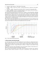
diesel engine A four-step cyclical engine, il-
lustrated below. It consists of an adiabatic com-
pression of the air and fuel mixture (i), followed
by a combustion step at constant pressure (ii),
and then cooled first by an adiabatic expansion
(iii), withfurther cooling atconstant volume(iv)
© 2001 by CRC Press LLC
to return the gas to the initial temperature and
pressure.
Diesel engine cycle.
difference frequency generation A non-
linear process in which radiation is generated
that has an energy equivalent to the difference
of the two initially present radiation fields. It is
the reverse process of sum frequency generation
and closely related to optically parametric down
conversion. Energy and momentum conserva-
tion have to be fulfilled in the process, i.e.,
ν
d
=ν
1
−ν

2
energy conservation ,

k
d
=

k
1
−

k
2
momentum conservation
where ν are the frequencies and

k are the wave
vectors of the different radiation fields involved.
differential cross-section The nuclear cross-
section per unit of energy, momentum, or angle;
usually refers to the angular differential cross-
section. The differential cross-section per solid
angle, ∂, is written as:
∂σ
∂
.
diffraction At forward angles and small mo-
mentum transfers, the scattering of high energy
particles from a composite of target scattering
centers, such as nucleons in a nucleus, is pri-

marily governed by the wave nature of these pro-
jectiles. Scattering from such a system can be
coherent, i.e., the incident and outgoing particle
waves are identical except for a phase change,
leading to a description of the scattering in terms
of interfering waves. Scattering represented by
this process is called diffractive scattering or
diffraction.
diffuser A duct in which the flow is decel-
erated and compressed. The shape of a diffuser
is dependent upon whether the flow is subsonic
or supersonic. In subsonic flow, a diffuser duct
has a diverging shape, while in supersonic flow,
a diffuser duct has a converging shape. See
converging–diverging nozzle.
diffusion The movement of a solid, liquid,
or gas as a result of the random thermal motion
of its atoms or molecules. Diffusion in solids is
quite small at normal temperatures.
diffusion coefficient, diffusion length Neu-
tronsabovethermalenergiesloseenergybyscat-
tering from the nuclei of a material, losing en-
ergyuntil theyare capturedbya nucleusor reach
thermal equilibrium with the surrounding envi-
ronment. Thus, the average energy of an initial
distribution of neutrons will decrease over time,
and the width will increase (diffuse):
D = λv/3 ,
where v/λ is the number of collisions of the
neutron per unit of time, and D is the diffusion

coefficient. The quantity,
L =[λ/3]
1/2
,
where /v isthe mean-lifeof athermalneutron,
is the diffusion length. The density of thermal
neutrons thenobeysthe equation(q
τ
the number
of neutrons becoming thermal per unit time),
∇
2
n − (3/λ)n + 3q
τ
/λv = 0 ;
with the boundary condition n = 0 on the sur-
face of the moderator.
diffusion, plasma The loss of plasma from
one region (normally the interior) to another
region (normally the exterior) stemming from
plasma density or pressure gradients.
diffusion, viscous Penetration of the effects
of motion in a viscous fluid where the bound-
ary layer grows outward from the surface. Near
© 2001 by CRC Press LLC
the surface, fluid parcels are accelerated by an
imbalance of shear forces. As the fluid moves
adjacent to the wall, it drags a portion of the
neighboring fluid parcels along with it, result-
ing in a gradual induction of fluid moving with

or retarded by the surface. In an unsteady flow,
the diffusion is governed by the simplified equa-
tion
∂u
∂t
=ν
∂
2
u
∂y
2
where viscous forces govern the fluid behavior.
dilatant fluid Non-Newtonian fluid in which
the apparent viscosity decreases with an increas-
ing rate of deformation. Also referred to as a
shear thickening fluid.
dimensional analysis The basis of dimen-
sional analysis is that any equation which ex-
presses a physical law must be satisfied in all
possible systems of units. What differentiates
between one set of units and another is how the
system is defined, in particular, what quantities
are chosen as primary. These are the basic set
of units. All other units are a combination of
these and are known as secondary (these are also
known as base and derived units when specifi-
cally referring to the system). In fluid mechan-
ics, the primary dimensions are usually mass,
length, time, and temperature (SI). All other
physical quantities are derived from these pri-

mary dimensions.
dimensionless intensity The intensity in
atomic units often used in theoretical calcula-
tions. In particular in the semiclassical theory,
a dimensionless intensity can be defined which
is equivalent to the number of photons n in the
laser mode with volume V :
n=

0
E
3
V
2
¯
hω
,
whereω is the angular frequency of the photons.
In the literature, the intensity is often defined
as:
I=
c
8π
E
2
,
where E is the time averaged electric field. The
standard SI unit for the intensity is W/m
2
. The

intensity is sometimes also referred to as the ir-
radiance.
dimensionless parameter Any of a number
of parameters characterized by value alone and
whichdescribescharacteristicphysicalbehavior
of fluid flow phenomena. A dimensionless pa-
rameter is composed of a ratio of two quantities
with the same dimensions to measure the rela-
tive effect of these quantities in a given flow (see
Reynolds number, Mach number). Some di-
mensionless parameters of common use in fluid
mechanics are listed below.
Name Form & Ratio
Cauchy number Ca =U
2
ρ/β
s
=M
2
inertia force:compressive force
Euler number Eu =p/ρU
2
pressure force:inertia force
Froude number Fr =U
2
/gL
inertia force:gravity force
Grashof number Gr =gβTL
3
/ν

2
buoyancy force:viscous force
Knudsen number K =λ/L
mean free path:length scale
Mach number M =U/a
velocity:sound speed
Reynolds number Re =UL/ν
inertia force:viscous force
Stokes number Sk =pL/µU
pressure force:viscous force
Strouhal number
St =fU/L
vibration frequency:time-scale
Weber number We =ρU
2
L/σ
inertia force:surface tension force
diode An electronic device that exhibits rec-
tifying action when a potential difference is ap-
plied between two electrodes. Current flows
from one direction of the potential, called the
forward direction. When the potential is re-
versed, the current is very small or zero.
dipolar force The attractive force between
two molecules originating from the polariza-
tion of the molecules. The partially positively
charged end of a molecule attracts the partially
negatively charged part of the other molecule.
dipole-allowed transition See electric
dipole-allowed transition.

dipole approximation Frequently used
when the interaction between an atom and an
electromagnetic wave is considered. The elec-
© 2001 by CRC Press LLC
tromagnetic wave can be written as the resultant
from a vector potential

A as

E
(
r,t
)
=−
1
c
∂
∂t

A
(
r,t
)

B
(
r,t
)
=∇×


A
(
r,t
)
.
An electron subject to the vector potential

A has
the minimal coupling Hamiltonian:
H =
1
2m

p −e

A

2
+ eU (r, t) + 
(
r
)
,
where

A and U are the vector and scalar poten-
tials of the field, and (r) constitutes the scalar
Coulomb potential. In the radiation gauge we
find
U = 0 and ∇


A = 0 .
Theinteractionofatwo-levelatomiswithspher-
ical waves that can be written with the help of
the vector potential as

A
(
r,t
)
=A
2
(t) exp

ı

kr

+A
2
(t) exp

−ı

kr

,
which gives rise to the interactions of the form

f

|
e
m
A
2
p exp

ı

kr

|
i

where the rotating wave approximation was as-
sumed. In the dipole approximation, one as-
sumes that the electric field of the wave (λ ≈
1000Å) does not significantly change across the
dimension of the nucleus λ ≈ 1Å. Mathemati-
cally it means that only the zeroth order term in
the series expansion for the operator
exp

ı

kr

= 1 + ı

kr +

1
2

ı

kr

2
+···
is used. Here,

k is the wave vector of the electro-
magnetic wave, and r is typically the extent of
the nucleus, i.e., in the order of 1 Å. There-
fore, the higher order terms are much smaller
than the leading term and the dipole approxima-
tion holds. Theseare the electricdipole-allowed
transitions (E1). Thus, using the dipole approx-
imation, the interaction betweenstates |
f
and
|
i
 can then be written as

f
|
e
m
p|

i
 ,
which, by means of a gauge transformation of
fields and wave functions to the electric field
gauge, can be shown to be equivalent to
ω
2
fi


f
|er

i
whereω
fi
istheresonancefrequencyofthetran-
sition.
In the case that the zeroth order term has no
contribution, i.e., in thecase ofdipole-forbidden
transitions, the higher order terms can become
important.
dipole field The field of an electric dipole
with dipole moment q

d.Itisgivenby

E
(
r

)
=
q
4πε
0
3


dr

r −
(
rr
)

d
r
5
.
dipole-forbiddentransitions Transitionsfor
which the electric dipole transition moment in
the dipole approximation vanishes:



1
|eˆr|
2




2
=




e


∗
1
r
2
dr




2
= 0 .
Transitions are possible due to higher order
terms in the expansion of the matrix element




1
|
e

m
e pe
ı

kr
|
2




2
which is derived considering interactions of one
photon with a two-level system using the radia-
tion gauge Hamiltonian. These transitions are
much weaker than dipole-allowed transitions.
The two most important types are magnetic
dipoleand electricquadrupoletransitions. Their
selection rules are:
magnetic dipole transitions:
J = 0, ±1
L = 0
m = 0, ±1
electric quadrupole transition:
L =±2
m = 0, ±1, ±2 .
One also speaks of forbidden transitions in
the case of intercombination lines, where the
© 2001 by CRC Press LLC
selection rule S= 0 is violated. This can be

the case for heavy atoms, where the spin–orbit
interaction is large. These transitions still have
dipole characteristics, since they occur due to
the admixture of other states to the bare states in-
volved in the transitions. An example is the well
known 253.7 nm transition in mercury (
3
P
1
←
1
S
0
).
dipole forces Result from the interaction of
the induced dipole moment in an atom or mol-
ecule with an intensity gradient of the light field
causing this dipole. Several models are avail-
able to describe the conservative dipole force.
In the oscillator model, we assume a two-level
system and use the rotating wave approximation
(assuming that the laser frequency detuning 
from the resonance at ω
0
is small compared to
the frequency ω
0
: ||<<ω
0
). Thus, the force

on a particle is
F(r)=−∇U
dipole
(r)=
3πc
2
2ω
3
0


∇I(r),
where ω
0
and  are the resonance frequency
of the atom, and the linewidth of the resonance
transition, and =ω−ω
0
is the detuning of
the laser from the resonance; c is the speed of
light. The force is conservative since it can be
written as the gradient of a potentialU
dipole
. The
heating of the sample due to absorption of the
light by the atomic system can be measured by
the scattering rate (r) of photons:
(r)=
3πc
2

2
¯
hω
3
0

2

2
I(r).
As indicated above, α is dependent on the fre-
quency of the light field.
It is important to realize the dependence of
the dipole force on the sign of the detuning. For
red detuning, i.e., <0, the force is negative.
The atoms or molecules are therefore drawn to
high intensities. For the case of blue detuning,
i.e., >0, the force is positive, and the inter-
action leads to a repulsion of the particles from
areas with high intensity.
The potential scales with I/, whereas the
scattering rate, i.e., the heating, scales with I/

2
. Thus, large detunings lead to much smaller
heating of the sample, but do require larger in-
tensities to produce the same force.
It should be noted that for multi-level atoms,
the expressions for the force and scattering rate
become slightly more complicated.

The dipole trap is based on dipole forces.
dipolemoment Associatedwithachargedis-
tribution (r), and given by
d=

d
3
rr=−e

d
3
r
n
(
r
)
∗
r
n
(
r
)
,
where e is the elementary charge and we have
used the relationship between the charge den-
sity  and the wave function 
n
of a stationary
electron:
r=−e

n
(
r
)
∗
r
n
(
r
)
.
dipole operator Defined as
ˆ
d=−er
where e is the elementary charge.
dipole selection rule States that electric
dipole transitions in any system take place be-
tween levels that differ by, at most, one unit of
angular momentum, except in the case where
both levels have zero angular momentum. Sim-
ilar rules accompany magnetic dipole and higher
multipole transitions.
dipole sum rule Rule that puts an upper
boundary on the total absorption cross-section
for any system in its ground state, under the as-
sumption that the absorption is primarily due to
dipole transitions. The rule is of value in esti-
mating transition matrix elements, and played a
historically importantrole inthe developmentof
quantummechanics. AlsoknownastheThomas-

Reiche-Kuhn rule.
dipole transition See electric dipole-allowed
transition; forbidden transition.
dipole transition moment For a one-elec-
tron atom between state 
n
and 
m
, the dipole
transition moment is defined as the integral
d =−e

d
3
r
m
(
r
)
∗
r
n
(
r
)
.
© 2001 by CRC Press LLC
The value |d|
2
is proportional to the transition

probability for an electric dipole transition be-
tween the two states 
n
and 
m
. It can be de-
rived from the zeroth order term of the series
expansion of the operatore
ı

kr
, which appears in
the interaction Hamiltonian. The dipole tran-
sition moment is derived with the help of the
dipole and rotating wave approximations.
dipole traps (optical dipole traps) Allow
trapping of neutral atoms and molecules. Their
action is based on the dipole forces in far-
detuned light. Typically, their trap depths
are much lower than those of the magneto-
optical traps or purely magnetic traps. They
are typically below 1 mK. Therefore, atoms or
molecules that are to be trapped in dipole traps
must be pre-cooled with other techniques before
they can be stored. However, since the trap-
ping mechanism is based on non-resonant light,
molecules as well as atoms can be trapped.
Dirac equation A quantum mechanical,
relativistic wave equation which describes the
interaction and motion of particles with an in-

trinsic spin of 1/2. The equation has the form:
Hψ=i
∂ψ
∂t
,
where the Hamiltonian for a free particle is writ-
ten as:
H=γ
4

γ
k
∂
∂x
k
+m

.
Theγ s are 4× 4 matrices, the wave function,ψ,
is a four-dimensional column vector, the two up-
per components represent the two spin states of a
positive energy particle, and the lower two com-
ponents represent the two spin states of the cor-
responding negative energy particle (anti-par-
ticle).
Diracholetheory Theoryinwhichthephysi-
cal vacuum is regarded as obtained by filling all
the negative energy single-electron states that
emerge as solutions of the Dirac equation, and a
positron is regarded as obtained by the removal

of one of the negative energy states.
Dirac magnetic monopole Particle postu-
lated by P.A.M. Dirac in 1931, which would
act as a source of magnetic flux density B in
the same way as an electron is a source of the
electric field E. Thus, an infinitesimal surface
enclosing a magnetic monopole would have a
nonzero magnetic flux passing through it. Dirac
showed that the magnetic charge g of such a
particle and the electric charge e of the electron
would be related by the so-called Dirac quanti-
zation condition, according to which the product
ge must be an integral multiple ofhc/4π, where
h is Planck’s constant andc is the speed of light.
No magnetic monoples have been discovered to
date. See also Dirac string.
Dirac matrix A four-dimensional matrix
which is a component of the Dirac equation and
which describes the operations of parity and
space–time rotations of the spin degrees of free-
dom. There are several representations of these
matrices, but one useful representation may be
written in terms of the Pauli spin matrices, σ.
Thus,
γ
k
=

0 −iσ
k

iσ
k
0

;
and
γ
4
=

10
0 −1

.
See Dirac equation.
Dirac notation A nomenclature to write
quantum mechanical integrals introduced by
Dirac. The expectation value for an operator
ˆ
A for a wave function  can be expressed in the
Dirac notation simply as
|
ˆ
A|=


∗
Adr,
where the Schrödinger notation is used in the
second part. The | and | parts are referred

to as bra and kets, respectively.
Dirac quantization condition See Dirac
magnetic monopole.
Dirac string A convenient representation of
the singularity that necessarily arises in describ-
ing a magnetic monopole in terms of a mag-
netic vectorpotential A. The total magnetic flux
emerging from the monopole is viewed as re-
turning to the monopole along a string of zero
© 2001 by CRC Press LLC
width anchored to the monopole. The string can
wind around arbitrarily in space, but cannot be
eliminated, reflectingthefactthat thesingularity
cannot be removed by any choice of gauge.
direct band gap semiconductor In a direct
band gap semiconductor, the conduction band
edge and valence band edge are at the center of
the Brillouin zone, such as GaAs, InSb, etc.
direct drive An approach to inertial con-
finement fusion in which the laser or particle
beam energy is directly incident on a pea-sized
fusion-fuel capsule resulting in compression
heating from the ablation of the target surface.
direct reaction Nuclear reactions are gen-
erally described as compound or direct. Al-
though this classification is not well-defined, a
compound reactionusually occurs at low energy
when a particle is absorbed by a nucleus, the in-
cidentenergyissharedby atleastseveralnuclear
components, andparticles areemitted to remove

the excess energy. A direct reaction usually oc-
curs at higher energy when an incident particle
interacts with one nuclear component, directly
producing thefinal nuclearstate withoutthe sys-
tem passing through a set of intermediate states.
discharge coefficient Empirical quantity
used in flow through an orifice to account for
the losses encountered in non-ideal geometries
from separation and other effects.
discrete spectrum A discrete set of values
in quantummechanics for theobservationalout-
comes (the spectrum) of a physical quantity, as
opposed to values that run through a continuous
range. For example, the spectrum of angular
momentum is wholly discrete.
dispersive wave A wave that propagates at
different speeds as a function of wavelength,
thus dispersing as the wave progresses in time
or space.
displacement thickness In boundary layer
analysis, the distance by which the wall would
have to be displaced outward to maintain the
identical mass flux in the flow, given by
δ
∗
=

∞
o


1 −
u(y)
U
∞

dy
where U
∞
is thefree-stream velocityoutside the
boundary layer.
disruption, or plasma disruption Plasma
instabilities (usually oscillatory modes) some-
times grow and cause abrupt temperature drops
andthe terminationofaexperimentallyconfined
plasma. Stored energy in the plasma is rapidly
dumped into the rest of the experimental system
(vacuum vessel walls, magnetic coils, etc.).
dissipation The transformationof kineticen-
ergy to internal energy due to viscous forces. It
is proportional to the square of the velocity gra-
dients and is greater in regions of high shear.
distorted wave approximation The transi-
tion matrix between two quantum mechanical
states can be expressed as:
S
fi
=

φ
f

|
H
int
|
ψ
i

;
where H
int
is the perturbing Hamiltionian that
causes the transition between the states, ψ
i
is a
state of the complete Hamiltonian, H = H
0
+
H
int
with initial boundary conditions, and φ
f
is a state of the unperturbed Hamiltonian, H
0
,
with final boundary conditions. In general, ψ
i
is difficult to determine and isreplaced by anap-
proximate wave function, usually found by per-
turbation techniques. Thus to first order when
ψ is replaced by φ

f
, one has the plane-wave
Born approximation. More realistic approxima-
tions may be determined by replacing the exact
Hamiltonian, H , with one which has an approx-
imate interaction potential, but is more easily
solvable, e.g., the addition of a Coulomb poten-
tial plus some central potential. Then the ap-
proximate ψ is not exactly correct but is more
realistic and is distorted from the plane wave
solutions, φ.
divergence operator The application of the
divergence operator on a vector field gives the
flux of that vector out of an infinitesimal volume
perunit ofvolume. In Cartesian coordinates, the
© 2001 by CRC Press LLC
divergence of a vector, A is written:
∇• A =
∂A
x
∂x
+
∂A
y
∂y
+
∂A
z
∂z
.

divergence theorem Relation between vol-
ume integral and surface integral given by

V
∇·QdV=

A
Q ·dA
where Q can be either a vector or a tensor. Also
referred to as the Gauss-Ostrogradskii diver-
gence theorem.
divertor, plasma divertor Component of a
toroidal plasma experimental device that diverts
charged ions on the outer edge of the plasma into
a separate chamber where charged particles can
strike a barrier and become neutral atoms.
D Meson Class of fundamental particles con-
structed of a charmed (anti-charmed) quark and
an up or down (anti-up or anti-down) quark. The
lowest representation of these mesons are the
D
±
and the D
0
, which have spin 0 and nega-
tive parity and are composed of c
dorcd and cu,
respectively.
domain In ferroelectric materials, there are
many microscopic regions. The direction of po-

larization is the same in one domain; however,
in adjacent domains, the directions of polariza-
tion are opposite.
donor levels The levels corresponding to
donors, found in the energy band gap and very
close to the bottom of the conduction band.
donors In a semiconductor, pentravalent im-
purities which can offer electrons are called do-
nors.
dopant See acceptor.
Doppler broadening The inhomogeneous
broadeningofa transitionduetothevelocitydis-
tribution of an ensemble of atoms. The broad-
ening comes from the Doppler detuning for in-
dividual atoms, which have different velocity
components with respect to the propagation di-
rection of the light. If the ensemble of atoms
exhibits a Maxwell-Boltzmann distribution for
their velocities, one finds a Doppler-broadened
line width of
ν =
2ν
0
c

2R ln 2
M
,
whereR isthegeneral gasconstant,M is themo-
lar mass, and λ and ν

0
are the resonance wave-
length and frequency, respectively.
Doppler detuning The detuning of a transi-
tioncausedby themovementoftheatom relative
to the source of radiation. Doppler detuning is
sometimes called the Doppler shift.
Doppler distribution The characteristic line
shape of a transition that is broadened due to the
movement of the atoms. Since each atom has
a different velocity and, consequently, a differ-
ent Doppler shift, one speaks of an inhomoge-
neous distribution. For atoms with a Maxwell–
Boltzmann distribution ofthe velocities, thedis-
tribution is given by a Gaussian profile:
I(ω)= I
0
exp

−

c
(
ω − ω
0
)
ω
0
v
m


2

,
where v
m
=

2kT
m
=

2RT
M
where ω
0
is the resonance frequency, v
m
is the
most likely velocity of the distribution, T is the
equilibriumtemperature oftheatoms, andm and
M are their atomic and molar masses, respec-
tively. k and R are the Boltzmann constant and
general gas constant, respectively.
However, experimentally, usually the convo-
lutionof aGaussian(inhomogeneous)with aho-
mogeneously broadened linewidth (collisions)
is observed:
I(ω)=
I

0
Nc
2v
m
π
3/2
ω
0

∞
0
exp

(
−c/v
m
)
2

ω
0
− ω


2
/ω
2
0

(

ω − ω

)
2
+ (/2)
2
dω

.
Here,  is the width of the Lorentzian profile.
This convoluted distribution is called the Voigt
profile.
Doppler-free excitation An excitation
method that circumvents the Doppler shift of
© 2001 by CRC Press LLC
the resonances due to the motion of the individ-
ual atoms so that for a given laser frequency, all
atoms will be excited. Examples are two-photon
spectroscopy and saturation spectroscopy.
In two-photon spectroscopy, the atom ab-
sorbs one photon out of each of two counter-
propagating beams. In this way, the Doppler
shift with respect to one beam is canceled by
the Doppler shift occurring with respect to the
second. Since there is a probability for the atom
to absorb two photons out of the same beam,
there will be a small pedestal underneath the
Doppler-free main signal.
In saturation spectroscopy, two laser beams
of different intensities — a strong pump and a

weak probe derived from the same laser beam —
are counterpropagated through a cell. The laser
beams are both intensity-modulated with differ-
ent frequencies. The laser is then tuned. Since
the Doppler shifts for both beams are opposite,
the probe signal will be modulated at the sum
of the two modulation frequencies only when
the two lasers interact with the same subclass
of atoms, i.e., atoms with no movement relative
to the pump and probe beam. Thus, the probe
signal measured via a lock-in amplifier will be
free of Doppler broadening.
Doppler limit The temperature limit in atom
trapping, which was originally considered the
limit for laser cooling of atoms. The limit is
reached when the natural line width of the cool-
ing transition reaches the Doppler shift associ-
ated with the movement of the atom. It is given
by
kT
Doppler
=
¯
h/2 ,
wherek is the Boltzmann constant,
¯
h is Planck’s
constant, and  is the line width of the cooling
transition. Experiments showed that atoms can
be cooled to much lower temperatures, which is

due to the internal structure, i.e., Zeeman sub-
levels, of the atoms. The latter cooling mecha-
nisms are referred to as sysiphus and polariza-
tion gradient cooling.
Doppler profile See Doppler distribution.
Doppler shift (1) When either the source or
the receiver is moving with respect to the ref-
erence frame in which a wave is traveling, the
wavelength (frequency) in that moving frame
will change. This is due to the obvious fact that
the spacing between wave crests will increase
or decrease due to relative motion between the
frames, and is known as the Doppler shift. Rel-
ativistically it is expressed as:
ν =
ν[1 −β cos(θ)]

1 − β
2
,
where β = v/c, and θ is the angle between the
wave vector and the velocity, v.
(2) The shift in the transition frequency of
an atom or molecule that occurs when an atom
is moving relative to the radiation source. The
transition is red-shifted if the atom moves to-
wards the source and blue-shifted if it moves
away. The shifted resonance frequency is given
by
ω

D
= ω
0
+

kv = ω
0

1 +
v
z
c

,
where ω
0
is the resonance frequency in the an-
gular frequency of the atom, and

k and v are
the wave vector of the light and the velocity of
the atom respectively. v
z
is the atomic velocity
component in the direction of light propagation.
Doppler width The broadened line width of
a transition caused by the random movement of
an ensembleof atoms. Theresonance frequency
of each atom is shifted due to the Doppler ef-
fect by a different amount corresponding to the

Doppler shift for its particular velocity. Assum-
ing a Boltzmann distribution for the velocities
of the atoms with mass m at temperature T , the
Doppler width has a value of
δν = 2
ν
0
c

2R ln 2/M =
2
λ

2R ln 2/M
where c is the speedof light, R is the general gas
constant, and M is the molar mass of the atom.
It is apparent that the Doppler width is propor-
tional to the transition frequency. Typically, the
Doppler width is twice that of the natural line
width for frequencies in the visible spectrum.
dose A measure of the exposure to nuclear
irradiation. It ismeasured inunits of6.24×10
12
MeV/kg (1 joule/kg) of deposited energy in the
material (gray). The older unit of dose, the rad,
© 2001 by CRC Press LLC
is 10
−2
gray. The gray does not include a factor
for biological damage which is dependent on the

type and energy of the radiation, w
R
. Thus, the
biological dose in sievert isSv= absorbed dose
in gray ×w
R
. See gray.
double beta decay A simultaneous change
of two neutrons into two protons. For a few nu-
clei, this may result in a lower mass nucleus, but
the original nucleus is stable against single beta
decay. There are 58 nuclei, all even–even (neu-
tron number–proton number), which can result
in double beta decay. As double beta decay is a
second order weak process, it is extremely rare,
and the lifetimes of these isotopes are ≥ 10
19
years. The process is of interest, however, be-
cause it is potentially possible for neutrino-less
beta decay to occur if the neutrino possesses cer-
tain properties. That is, instead of the process
Z
X
A
→
Z+2
X
A
+ 2e
−

+ 2ν;
one could have the reaction
Z
X
A
→
Z+2
X
A
+ 2e
−
.
This latter process violates lepton conservation,
but aside from that, the latter process occurs with
much higher probability than the former pro-
cess. Thus, neutrino-less beta decay is a sensi-
tive test of lepton conservation, and, in particu-
lar, of whether the emitted neutrino is a Majo-
ranaoraDiracparticle, i.e., whethertheneutrino
is its own anti-particle.
double escape peak In the interaction of a
photon with a nucleus, the creation of electron–
positron pairs is possible if the photon, has en-
ergy above two electron masses. To determine
the energy of the original photon, all the de-
posited energy must be measured, and this in-
cludes the capture of the two annihilation pho-
tonsof0.511MeVeach, emittedwhenapositron
at rest captures an electron. If these secondary
photons escape the detector, then the measured

energy of the photon is reduced by 0.511 or 2 ×
0.511 = 1.022 Mev, depending on whether one
or two photons escape. This produces a full en-
ergy peak (no escape), a single escape peak, and
a double escape peak in the measured energy
spectrum.
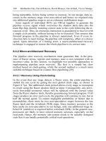
double resonance spectroscopy A tech-
nique often used in atomic and molecular spec-
troscopy. Molecular spectra usually show spec-
tral congestion, and the multitude of lines makes
their assignment difficult. At a high density of
states, the lines might even overlap. Using dou-
ble resonance techniques can greatly reduce this
congestion, since the second resonant light pro-
vides additional selection. One distinguishes
between RF/optical, microwave/optical, and op-
tical/optical double resonance depending on the
frequency range used. Other distinguishing fea-
tures are the arrangement of the energy levels
involved, as depicted in the figure. Usually the
pump laser is fixed at a particular resonance fre-
quency, while the other laser is tuned.
Double resonance schemes distinguished by the ar-
rangement of the energy levels:
λ-type, V -type, and
step-wise.
double-slit experiment Classic experiment
first performed by Thomas Young in 1801, in
which light from a source falls on a screen af-
ter passage through an intervening screen with

two close-by narrow slits. Under suitable con-
ditions, a pattern of alternating dark and bright
fringes (images of the slit) appears on the final
screen. This experiment was the first to demon-
strateconvincinglythe wavenature oflight. The
same experiment may be done (with inessential
modifications) with sound, X-rays, electrons,
neutrons, or any otherparticle, as a consequence
of de Broglie’s principle. See diffraction.
doublet A dipole in potential flow consist-
ing of a source and sink of equal strength and
infinitesimal separation between them. The
streamfunction  and velocity potential φ are
given by
 =−
K sinθ
r
© 2001 by CRC Press LLC
and
φ=−
K cosθ
r
where K is the strength of the doublet. In a
superimposed uniform flow, a closed streamline
is formed around the doublet. Doublets can be
used in potential flow to simulate the flow past
a body such as flow past a cylinder (doublet in
uniform flow) or flow past a rotating cylinder
(doublet with superimposed vortex in uniform
flow).

down-conversion A non-linear process in
which, due to the non-linear interaction of a
pump photon with a medium, two photons of
lowerenergyaregenerated. Itisoftenreferredto
as parametric down-conversion. Down-conver-
sion is closely related to difference frequency
generation. The generated photons are the sig-
nal (higher energy) and the idler photons. En-
ergy and momentum have to be fulfilled in the
process, i.e.,
ω
p
=ω
s
+ω
i

k
p
=

k
s
+

k
i
,
where ω and


k denote the respective frequen-
cies and wave vectors. The efficiency of the
process is larger when the process is collinear,
i.e., all wave vectors are either parallel or anti-
parallel. Generally, the process can take place
only in birefringent media, because otherwise
the phase-matching condition can not be met.
With the exception of processes in periodically
poled media, this requires that some of the three
involved photons differ in polarization. One
must distinguish between type-I and type-II pro-
cesses. In type-I processes, the idler and signal
photons have the same polarization, while for
type-II processes they are perpendicular to each
other. Parametric down-conversion processes
are used to build optical parametric oscillators.
Parametric down-conversion can be used to
produce squeezed light and entangled states be-
tween photons.
TheHamiltonianintherotatingwaveapprox-
imation in the interaction picture is written as
H
int
=
¯
hκ

a
†
s

a
†
i
a
p
+a
s
a
i
a
†
p

,
where κ is the coupling constant, a
s
, a
i
, and a
p
are the annihilation operators, and a
†
s

, a
†
i

, and
a

†
p

are the creation operators at the respective
frequencies. The coupling constant is among
others on the second order susceptibility tensor
of the non-linear material used in the non-linear
process. Often the processes are studied under
the parametric approximation, where the pump
field is treated classically. Consequently, one
also assumes that the pump field is not depleted.
In this case, the Hamiltonian is written as:
H
int
=
¯
hκβ

a
†
s
a
†
i
e
−ı
+a
s
a
i

e
ı

.
down quark Fundamental hadronic particles
are composed of quarks and anti-quarks. In the
standard model, the quarks are arranged in three
families, the least massive of which contains
quarks of up and down types. Nucleons are
constructed from a combination of three con-
stituent up and down quarks and a sea of quark–
antiquark pairs. Thus, a neutron has two down
quarks and one up quark, while a proton has
two up quarks and one down quark. The down
quark has -1/3 of the electronic charge and the
up quark has 2/3 of the electronic charge.
downwash Downward flow behind a wing
created as a direct result of the generation of
lift. See trailing vortex wake.
drag Resistive force opposed to the direc-
tion of motion. Drag can be generated by var-
ious forces including skin friction and pressure
forces. Drag is primarily a viscous phenome-
non (see D’Alembert’s paradox) with boundary
layers and separation as its primary causes.
drag coefficient Non-dimensionalized drag
force given by
C
D
=

D
1
2
ρU
2
∞
c
2
where c is the chord length of the airfoil. Drag
is used in
conjunction with lift to determine the effi-
ciency of the airfoil.
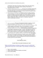
Drell–Yanprocess In nucleon–nucleonscat-
tering, the production of lepton pairs with high
transverse momentum far from a vector meson
© 2001 by CRC Press LLC
resonance is assumed to proceed by quark–anti-
quark annihilation. This first order process pro-
duces a virtual photon which converts into a lep-
ton pair in the final state. Thus, the Drell–Yan
process provides a mechanism to study the par-
ton distributions in nuclei.
A flow diagram of the Drell–Yan process. The quark–
antiquark annihilate to form a muon pair.
dressed atom Description of an atomic or
molecular system interacting with a quantized
radiation field in a coupled atomic-field basis.
Each energy state in this picture is expressed as
an atomic excitation and a specific number of
photons associated with it (see dressed states).

dressedstates The eigenstatesfor the Hamil-
tonianof anatomic ormolecular systemcoupled
to a quantized radiation field. The discussion is
restricted here to two-level atoms with a ground
state |a and an excited state |b. For this two-
levelsystem, theHamiltonian usingthestandard
annihilation and creation operators can be writ-
ten in the rotating wave approximation as
H = H
A
+ H
F
+ H
AF
=
¯
hω
0
|bb|+
¯
hω
F

c
†
c +
1
2

+

¯
hg

c
†
|ab|+c|ba|

,
where H
A
=
¯
hω
0
|bb| is the Hamiltonian of
the atom with eigenstates |b and |a with ener-
gies
¯
hω
0
and 0 respectively. H
F
=
¯
hω
F
(c
†
c +
1

2
) is the Hamiltonian of the field, where c
†
and c are the creation and annihilation opera-
tors for a photon with frequency ω
F
. The term
H
AF
=
¯
hg(c
†
|ab|+c|ba|) is the interaction
between the field and the atom, where g is the
coupling constant. Without the coupling term
H
AF
, the eigenstates of the atom-field system
are two infinite ladders with |a, n and |b, n,
i.e., states where the atom is in the ground state
and n photons in the field and the atom is in the
excited state and n photons in the field. As de-
picted in the figure, the total energy of these
states is given by n
¯
hω and
¯
hω
0

+ n
¯
hω
F
re-
spectively. The interaction of Hamiltonian cou-
ple states with |a, n and |b, n − 1 leads to
new eigenstates, the perturbed states or dressed
states. The matrix element of this coupling is
given as
v =b, n − 1|H
AF
|a, n=g
√
n =
¯
h/2
 is called the Rabi frequency. The dressed
states have the form
|+(n)=sin θ|a, n+cos θ|b, n − 1
|−(n)=cos θ|a, n−sin θ|b, n −1 ,
where tan 2θ =−


, and  = ω
0
− ω
F
is the
detuning of the photons from the atomic res-

onance. The energy difference between these
states is given by
E =
¯
h

=


2
+ 
2
,
whichmeansthat for thecaseofweakexcitation,
( ≈ 0) the states go over in the unperturbed
states with an energy separation equivalent to
the detuning. θ takes on the value π/4 for the
case of no detuning, i.e.,  = 0. Thus, we find
that for the dressed states:
|+(n)=
1
√
2
(|a, n+|b, n −1)
|−(n)=
1
√
2
(|a, n−|b, n −1),
The dressed state description is valuable in un-

derstanding phenomena such as the Autler–
Townesdoubletin theemission ofdressedthree-
state atoms and the Mollow spectrum of the
emission of a coherently driven two-level atom.
drift chamber A type of multiwire parti-
cle detector which uses the time that it takes an
ionization charge to drift to its sense wires to
interpolate the position of the track between the
wires. A cross-sectionof atypical driftchamber
is shown in the figure. Generally, ions drift at
a velocity of ≈ 5 cm/µs, so with a typical time
resolution of ≈1 ns, a position resolution of100
µm can be obtained.
© 2001 by CRC Press LLC
Depiction of the unperturbed and dressed states for an
atom-field system.
Cross-section of a drift chamber. The drift wires and
foils shape the electrostatic field lines along which the
ionization charge drifts.
drift motion Charged particles placed in a
uniform magnetic field will have orbits that can
be described as a helix of constant pitch, where
the center axis of the helix is along the mag-
netic field line. However, if the magnetic field is
not uniform, or if there are electrical fields with
perpendicular components to the magnetic field,
then the guiding centers of the particle orbits
will drift (generally perpendicular to the mag-
netic field).
drift-tube accelerator A linear accelerator

thatusesradio-frequencyelectromagneticfields.
Theacceleratoriscomposedofconductingtubes
separated by spatial gaps. The rf-field is im-
posed in the gaps between the tubes and is ex-
cluded from the interior of the conducting tubes.
Thus, the particles drift, field-free, while the rf-
potential polarity opposes acceleration, and are
accelerated between the gaps during the other
half-cycle of the rf-fields.
drift velocity The drift velocity of an ion-
ization charge in a typical chamber gas is about
5cm/µs. The addition of an organic quenching
gas not only provides operational stability of the
wire chamber, but keeps the drift velocity of the
ionization more or less constant, independent
of the applied electric field in the wire chamber.
This fortuitous circumstance makes the position
vs. drift time function nearly linear in most sit-
uations.
drift waves Plasma oscillations arising in
the presence of density gradients, such as at the
plasma’s surface.
duality, wave-particle The observation that
quantum mechanical systems can exhibit wave-
and particle-like behavior. The wave-particle
duality is an independent principle of quantum
mechanics and not a consequence of Heisen-
berg’s uncertainty principle. The occurrence of
wave-like behavior can be understood through
the interference of indistinguishable paths of a

system from one common initial state to a par-
ticular final state. Particle-like behavior occurs
when this indistinguishability is destroyed and
which-path information becomes available. It
can be shown that the relationship
D
2
+V
2
< 1
exists, where V is the visibility of the interfer-
ence fringes defined as
V =
I
max
− I
min
I
max
− I
min
and D is a measure of the ability to distinguish
between paths. Whether particle or wave nature
is observed depends on the type of experiment
performed. If the experimentaims atwaveprop-
erties, those will be observed and particle fea-
tures likewise.
duct flow See pipe flow.
dusty plasma An ionized gas containing
small particles of solid matter which become

electrically charged. Particles may be dielectric
© 2001 by CRC Press LLC
or conducting and typically range in size from
nanometers to millimeters. Dusty plasmas oc-
cur in astrophysics plasmas, plasma processing
discharges, and other laboratory plasmas. Dusty
plasmas are sometimes called complex plasmas
and, when strongly-coupled, plasma crystals.
dynamic pressure The pressure of a flow at-
tributed to the flow velocity defined as
1
2
ρU
2
∞
.
See Bernoulli’s equation and pressure, stagna-
tion.
dynamic similarity When problems of sim-
ilar geometry but varying dimensions have sim-
ilar dimensionless solutions. See dimensional
analysis.
dynamic Stark shift The shift in the atomic
energy due to the presence of strong radiation
fields. The shift can be explained with the help
of the dressed state model. The ground and ex-
cited states of a two-level atom can be written as
|g, n and |e, n, where n is the number of pho-
tons. In the weak field limit, i.e., n ≈ 0, we can
neglect the photon number. For strong fields,

however, the levels |g, n and |e, n transform
into the dressed states
|e, n→|+,n+ 1=cos θ
n+1
|e, n
− sin θ
n+1
|g, n +1
|g, n→|−,n=cos θ
n
|g, n
− sin θ
n
|g, n −1 ,
where tan 2θ
i
=

i

with 
i
is the Rabi fre-
quency and  = ω − ω
0
is the detuning
between the radiation and the atomic resonance
transition. This transformation shifts the energy
levels of the states |e, n by +δ and |g, n by
−δ, known as the dynamic Stark shift. It is also

referred to as the light shift, since it depends on
the Rabi frequency  and, hence, on the light
intensity. The value of δ is given by
δ =
1
2



2
+ 
2
− 

.
Thedynamic Stark shiftissometimes alsocalled
the AC Stark shift due to its analogy to the Stark
shift of atomic levels in DC fields.
Dyson’s equations In quantum field theory,
formally exact integral equations obeyed by
propagators or Green’s functions in a system of
interacting fields. First obtained by F.J. Dyson
in 1949 in the study of quantum electrodynam-
ics.
Dyson series Perturbative expansion of any
Green’sfunctionor correlationfunction inanin-
teracting quantum field theory as a sum of time-
ordered products. First developed by F.J. Dyson
in 1949.
dysprosium An element with atomic num-

ber (nuclear charge) 66 and atomic weight 162.
50. The element has 7 stable isotopes. Dyspro-
sium has a large thermal neutron cross-section
and is used in combination with other elements
in the control rods of nuclear reactors.
© 2001 by CRC Press LLC
E
e Symbol commonly used for the elementary
charge:
e= 1.602176462(63)× 10
−19
C .
echo, photon Technique analogous to spin
echoes, in which the washing out of Rabi oscil-
lations by inhomogeneous broadening in a vapor
of atoms is partially reversed by a suitable pulse
at the resonant frequency.
echo, spin Ingenious technique invented in
1950 by E.L. Hahn, in which the damping of
the free induction decay signal in an NMR ex-
periment on a macroscopic sample, which arises
from the inhomogeneity of the local magnetic
fields experienced by the various nuclei, is re-
versed. In the simplest form, a so-calledπ-pulse
of radiation at the Larmor frequency of the nu-
clei is applied, reversing nuclear motion in such
a way as to rephase the nuclei after an interval.
The echo signal provides valuable information
about the interaction of the nuclear spins and
by extension, the atoms with their surround-

ings. Many sophisticated echo protocols now
exist, and the resonant echo technique is now a
standard tool of analysis in many branches of
physics. See also photon echo.
Eckert number E
c
A dimensionless param-
eter that appears in the non-dimensional energy
equation. The Eckert number is given as the
ratio U
2
/c
p
T , where c
p
is the specific heat
at constant pressure and T is a characteristic
temperature difference. It thus represents the
ratio of kinetic to thermal energy. The Eckert
number is the ratio of the Brinkman number to
the Prandtl number. The Brinkman number rep-
resents the extent to which viscous heating is
important relative to heat flow due to tempera-
ture difference. The Prandtl number is the ratio
of kinematic viscosity to thermal diffusivity and
represents the relative magnitudes of diffusion
of momentum and heat in a fluid. For fluids
with constant specific heats c
p
and c

v
, the Eck-
ert number is related to the Mach number, Ma,
by Ec = (γ −1)Ma
2
, whereγ is theratioc
p
/c
v
with c
v
representing the specific heatat constant
volume.
eddy A loosely defined entity in a turbulent
flow that is usually associated with a recogniz-
able shape, such as avortex, or a mushroom, and
a sizesuch as a wavelengthrange. Eddies do not
exist in isolation. Smaller eddies usually exist
with larger ones. One characteristic of turbu-
lent flows is the continuous distribution of eddy
sizes. The eddy size affects many phenomena,
such as diffusion and mixing.
eddy current Electrical current induced in a
conductingmaterial submittedtoa varyingmag-
netic field.
eddy viscosity Turbulent flows are charac-
terized by spatial and temporal fluctuations of
the velocity components. These fluctuations are
responsible for the exchange of energy and mo-
mentum among turbulence scales or eddies.

This exchange results in reduction of momen-
tum gradientssimilar to, yetmore effectivethan,
reduction of these gradients by molecular in-
teractions caused by viscosity. By analogy to
Newton’s law ofviscosity, eddyviscosity is used
to represent the effects of momentum exchange
between turbulence scales. The contribution of
this exchange to the mean flow is represented
by the Reynolds stress tensor written as ρ
u
i
u
j
.
This term appears in the time-averaged equa-
tion of motion. Consequently, eddy viscosity is
used to model turbulence. Eddy viscosity mod-
els include zero-, one-, and two-equation mod-
els. These models work well for non-separating
near-parallelshear flows. In order toapply them
to otherflows, correctionterms areusually used.
Eddy viscosity modeling has been used to solve
a variety of problems and is used in commer-
cial fluid software packages as well. Yet, with
the advancements in computing capabilities, di-
rect numerical simulation (DNS) and large eddy
simulation (LES) are becoming more common
methods in numerical studies of turbulent flow
fields.
© 2001 by CRC Press LLC

edge dislocation Two-dimensional defect in
a solid.
effective charge In many nuclear models,
the description of the properties of a many-body
quantum-mechanical state may be considered
in terms of a single particle moving in some
type of potential well created by other parti-
cles. However, this single particle may be as-
signed an effective mass and charge to better
fit the observed experimental data. For exam-
ple, in single-particle nuclear transitions with
the emission of a gamma ray, the remaining nu-
cleons also move about the system center-of-
mass. This motion can be taken into account in
a simple single-particle model by reducing the
charge of this particle.
effective field Electrical field created by an
effective charge.
effective mass Individual nucleons in a nu-
cleuscanberepresented, inmanycircumstances,
as though they possess the same properties as
free neutrons or protons. However, there is still
a residual interaction between the nucleons, and
this residual interaction can, for some applica-
tions, be approximated by the insertion of an
effective mass and charge for this particle. See
effective charge.
effective range Angular momentum in the
scattering of particles (e.g., nucleons) can be ig-
norediftheincidentenergyissufficientlylow(s-

waves). In this situation, information about the
scattering potential is contained in the asymp-
totic scattering wave function, which is basically
an outgoing wave, phase-shifted by the scatter-
ing potential. The s-wave phase shift can be
expanded in powers of 1/kR, where R is the ef-
fective range and k is the momentum of the par-
ticle in units of
¯
h. For uncharged particles this
expression is
kcot(δ)=−1/a+

k
2
R

/2 .
In this expression, a is the scattering length.
effective range formula Formula of gen-
eral validity that represents quantum mechanical
scattering at low energy in terms of just two pa-
rameters, the scattering length, and the effective
range. While the former is often not a length
characterizing the scattering potential, the latter
is, especially if the potential is attractive.
efficiency of an engine (η) The ratio of the
work output to the heat input in an engine. For a
Carnot cycle, the efficiency η equals 1−T
c

/T
h
,
where T
c
denotes the temperature of the cold
reservoir to which the energy exhausts heat, and
T
h
is the temperature of the hot reservoir from
which the energy extracts heat.
effusion The flow of gas molecules through
large holes.
Ehrenfest equation The equation of motion
that the quantum mechanical expectation values
of operators follow. In the case of the space
operator ˆx and the momentum operator ˆp,we
find the following Ehrenfest equations:
d
dt

ˆx(t)

=

∂H
∂p

d
dt


ˆp(t)

=−

∂H
∂x

,
where H is the Hamiltonian of the system and
· indicates the expectation value. Those equa-
tions are equivalent to the classical equations of
motions.
Ehrenfest’stheorem Statesthat thequantum
mechanical expectation values follow classical
equations of motion, the Ehrenfest equations.
eigenfunction See eigenvalue problem.
eigenstates Eigenstates of an operator
ˆ
A are
states | that obey the equation
ˆ
A|=c
i
| ,
where c
i
is a complex number. Any quantum
mechanical system in a state | can be ex-
pressed as a superposition of eigenstates, i.e.,

|=

i
a|
i

providedthesestates|
i
forma completebasis.
The latter condition can be expressed as

i
|
i

i
|=1 .
© 2001 by CRC Press LLC
A weight diagram of the baryon and meson octets,
which is the lowest representation of the SU(3) group
symmetry representing these particles.
Einstein A coefficient Gives the probability
for the spontaneous decay of an excited atom or
molecule. For different types of transitions, the
Einstein coefficient is given by
A
ν
=
16π
3

ν
3
3ε
0
hc
3
g
2
S
ed
electric dipole transitions
A
ν
=
16π
3
µ
0
ν
3
3hc
3
g
2
S
md
magnetic dipole transitions
A
ν
=

8π
5
ν
5
5ε
0
hc
5
g
2
S
eq
electric quadrupole transitions
where the subscript denotes that A is given in
Hz, ν is the frequency of the transition in Hz, ε
is the susceptibility of the vacuum, h is Planck’s
constant, c is the speed of light, and S
ed
, S
md
,
and S
eq
are the line strengths for electric dipole,
magnetic dipole, and electric quadrupole transi-
tions.
The relationship between the lifetime τ of a
state and the Einstein A coefficient is given by
A
ν

=
1
2πτ
,
where we assume that A is given in terms of ν.
If it is given in terms of the radial frequency ω,
we find
A
ω
=
1
τ
.
Finally the Rabi frequency  can be calcu-
lated using the Einstein A coefficient:
||
2
=
λ
3
4π
2
¯
hc
g
2
IA ,
where g
2
is the degeneracy factor of the upper

level, λ is the wavelength of the laser, and I the
intensity in W/m
2
.
Einstein A and B coefficients.
In case a level can decay to several states,
the Einstein A coefficient is given by the sum of
the individual Einstein A coefficients A
i
of the
decays to the individual levels.
Einstein, Albert Nobel Prize winner in 1905
for explaining the photoelectric effect. He is
better known for his theories of special and gen-
eral relativity. The general theory of relativity
was the first fully developed field theory which
provided the intellectual stimulation for modern
theoretical physics.
Einstein B coefficient Coefficient for ab-
sorptionor stimulatedemissionofa photonfrom
a level 1 to a level 2. If level 2 is higher in en-
ergy than level 1, the coefficient of stimulated
emission B
21
and stimulated absorption B
12
are
given by
B
12

=
g
2
g
1
B
21
A
21
=
8πhν
3
c
3
B
21
,
where A
21
is the Einstein A coefficient for the
transition from 2 →1, and g
2
and g
1
are the sta-
tistical weights or degeneracy factors for level 2
and 1,respectively. ν is the transitionfrequency.
The Einstein B coefficient can also be ex-
pressed in terms of the oscillator strength f of
the transition:

B
21
=
g
1
g
2
e
2
4mε
0
hν
f,
whereε is thedielectricconstant forthevacuum.
Einstein equation Equation announced by
Einstein in the form E = mc
2
, where E is en-
ergy, m is mass, and c is the speed of light.
© 2001 by CRC Press LLC
Einstein–Podolsky–Rosen experiment In-
troduced as a gedanken experiment by Einstein,
Podolsky, and Rosen in 1935. The authors
wanted to illustrate the incompleteness of quan-
tum mechanics.
The history of the Einstein–Podolsky–Rosen
experiment dates back to the early years of quan-
tum mechanics. Despite its successes in pre-
dicting the outcome of experiments, many felt
that quantum mechanics was an unsatisfactory

theory due to its counterintuitive nature, i.e.,
action-at-a-distance. Among the most promi-
nent critics were Einstein, Podolsky, and Rosen,
who expressed their concerns in an article en-
titled “Can Quantum Mechanical Description
of Physical Reality Be Considered Complete?”
publishedin1935in Phys.Rev. Theyintroduced
the EPR gedanken experiment to demonstrate
their belief that quantum mechanics was incom-
plete. Crucial to their discussion was the con-
cept of entanglement between particles, since
entangled states seemingly allow action-at-a-
distance. The gedanken experiment involved
the generation of a two particle system in an
entangled state, separation of the constituents,
and measurement of the correlations between
the entangled quantities. The original gedanken
experiment focused on an entanglement in space
and momentum. The most common referenced
version was introduced by D. Bohm and is based
on an entanglement between two spin 1/2 parti-
cles.
Einstein, Podolsky, and Rosen left open the
question of whether a complete description of
reality was possible. Later such complete the-
ories, which are classical in nature, were called
local hidden variable (LHV) theories. Hidden
variables were supposed to be the origin of the
observed correlations, resolving the “spooky”
action-at-a-distance.

For a long time, the discussions were only
philosophical in nature. This changed in 1964,
when J.S. Bell realized that LHV theories were
at least possible. This contrasts with von Neu-
mann’s proof that it was not possible to construct
LHV theories, which reproduced all the quan-
tum mechanical predictions. Bell showed that
von Neumann had been much too restrictive in
his expectations for LHV theories. In addition,
Bell showed that the statistical predictions of
these theories showed correlations which were
limited by an inequality. However, it was pos-
sible to find cases in which the statistical pre-
dictions of quantum mechanics violate this in-
equality. So for the first time, it was possible, at
least in principle, to distinguish between quan-
tum mechanics and its classical counterparts —
the local hidden variable theories.
A test of a Bell inequality involves the
measurements of correlations in an entangled
state, i.e., polarization or spin components with
respect to different axes. Of course, there
have been tests of the Bell inequalities before.
Among the more prominent tests are cascade de-
cay and down-conversion experiments. In the
former, the entanglement between a photon pair
is produced by a consecutive cascade decay in
an atom. In the latter, the entanglement between
the polarization of two photons is generated by
a non-linear process.

However, all previous tests of a Bell inequal-
ity have loopholes. Specifically, these are the
detection efficiency loophole and the locality
loophole. Due to low detection efficiencies in
previous photon-based experiments, additional
assumptions had to be introduced in order to de-
rive a testable Bell inequality. Thus, the result-
ing experiments test much weaker forms of the
Bell inequalities. In order to enforce the locality
condition, the detector for one particle should
not know the measurement orientation of the
other detector. This means that within the time
of the analysis and detection step at one detec-
tor, no information about its particular direction
can reach the other detector. The enforcement
of this condition not only requires large detector
distances, but also rapid, randomized switching
of the measurement directions. This was not the
case in the only previous experimental attempt
to enforce the locality condition.
einsteinum A transuranic element with
atomic number (nuclearcharge)99. Twenty iso-
topes have been produced, with atomic number
252 having the longest half-life at 472 days.
EIT See electromagnetically induced trans-
parency.
Ekman layer A boundary layer affected by
rotation. Ekman layers develop in geophysical
situations under the action of the Coriolis force.
© 2001 by CRC Press LLC

Outside the earth’s boundary layer, the flow is
approximately horizontally homogeneous. In
addition, the shear stresses are negligible. Con-
sequently, the Coriolis force balances the pres-
sure forces, i.e.,
f
c
U
g
=−
1
ρ
∂P
∂y
and
f
c
V
g
=
1
ρ
∂P
∂x
where U
g
and V
g
are the x and y components of
the geostrophic wind (wind outside the earth’s

boundary layer). The parameter f
c
is the Cori-
olis parameter and is equal to 2ω sin φ, where
ω = 2π/24 hrs = 7.27 × 10
−5
s
−1
and φ is the
latitude. Based on the balance between Coriolis
and pressure forces, the geostrophic wind is par-
allel to the isobars. Inside the earth’s boundary
layer, or in the Ekman layer, shear stresses must
be considered in the equation of motion to yield
f
c
U =−
1
ρ
∂P
∂y
−
∂
v

w

∂z
= f
c

U
g
−
∂
v

w

∂z
or
f
c

U
g
− U

−−
∂
v

w

∂z
= 0
and
−f
c
V =−
1

ρ
∂P
∂x
−
∂
u

w

∂z
=−f
c
V
g
−
∂
u

w

∂z
or
f
c

V
g
− V

+

∂
u

w

∂z
= 0 .
Thus, in the boundary layer, the balance is be-
tween pressure, Coriolis, and friction forces.
The pressure forces retain the same direction
and magnitude as in the outer layer. The fric-
tion force is in the opposite direction of the ve-
locity. Because the sum of the Coriolis and
friction forces must balance the pressure force,
the velocity vector must change directions. In
the Northern Hemisphere (where f
c
is positive),
the velocity vector is rotated to the left of the
geostrophic wind vector. Ekman layers also ex-
ist in oceans, but with different boundary con-
ditions than the atmosphere.
Ekman number A dimensionless parame-
ter that represents the relative importance of the
viscous forces associated with fluid motionsand
the Coriolis force. It is written as E = ν/L
2
,
whereν is thekinematicviscosity,  is theangu-
lar velocity, and L isa characteristic length. The

Ekmannumber is equaltotheratio oftheRossby
number (Ro = U/L), which is a measure of
relative importance of fluid acceleration to the
Coriolis acceleration, to the Reynolds number
Re = UL/υ, which is a measure of the relative
importance of inertia to viscous forces.
elastic collision A collision between two or
more bodies in which the internal state of the
bodies is left unchanged, i.e., energy is not con-
verted to or from heat or any other internal de-
gree of freedom.
elastic constants Hooke’s law states that for
sufficiently small deformations, the strain is di-
rectly proportionalto thestress, so thatthe strain
components are linear functions of the stress
components. The coefficient for strain compo-
nents in each direction are called elastic compli-
ance constants or elastic constants.
elasticity The property of a material of re-
turningof itsoriginaldimensionsafter adeform-
ing stress has been removed. A material sub-
jected to a stress produces a strain. The limit up
to which stress is proportional to strain (which
is called Hooke’s law) is called the elastic limit.
Beyond theelastic limit, the material will not re-
turn to its original condition (i.e., the stress is no
longer proportional to the strain) and permanent
deformation occurs.
elastic light scattering The scattering of
light in which the frequency of the scattered

light is not changed. Examples of this type of
processare Rayleighscattering orresonanceflu-
orescence.
elastic limit The minimum stress that pro-
duces permanent change in a body.
elastic modulus The ratio of elastic stress to
elastic strain on a body. There are three types of
elastic moduli depending on the types of stress
applied. Young modulus refers to tensile stress,
bulk modulus refers to overall pressure on the
© 2001 by CRC Press LLC