High Temperature Strain of Metals and Alloys Part 5 pdf
Bạn đang xem bản rút gọn của tài liệu. Xem và tải ngay bản đầy đủ của tài liệu tại đây (228.19 KB, 15 trang )
56 4 Physical Mechanism of Strain at High Temperatures
Fig. 4.11 The jog formation in a dislocation emitted by a
low-angle sub-boundary. (a) The initial position,
b
i
are the
Burgers vectors;
ξ
i
are the unit dislocation vectors. (b) The
same as (a) after changing the signs of the vectors
ξ
3
and
ξ
4
. P
1
and P
2
are the slip planes;
V
1
and
V
2
are the velocity
vectors. (c) Dislocations with jogs after emission of the
dislocation
ξ
1
.
The typical Burgers vectors, slip planes and unit dislocation vectors have
been selected for examination of sub-boundaries. The results are presented
in Table 4.2. The angles <
b
1
ξ
1
and <
b
2
ξ
2
are not equal to 90
◦
. This means
that the dislocations of both systems contain screw components.
Tab. 4.2 The crystallography of low-angle sub-boundaries.
Lattice Slip <ξ
1
ξ
2
b
1
ξ
1
<b
1
ξ
1
b
2
ξ
2
<b
2
ξ
2
plane
f.c.c. {111} 90
◦
a
2
[110]
√
2
2
[110] 0
◦
a
2
[
¯
110]
√
2
2
[
¯
110] 0
◦
60
◦
a
2
[110]
√
2
2
[110] 0
◦
a
2
[10
¯
1]
√
2
2
[10
¯
1] 0
◦
60
◦
a
2
[011]
√
2
2
[
¯
1
¯
10] 120
◦
a
2
[
¯
110]
√
2
2
[0
¯
11] 120
◦
60
◦
a
2
[110]
√
2
2
[110] 0
◦
a
2
[
¯
110]
√
2
2
[011] 60
◦
b.c.c. {110} 90
◦
a
2
[111]
√
2
2
[110] 35.3
◦
a
2
[1
¯
11]
√
2
2
[1
¯
10] 35.3
◦
73.2
◦
a
2
[111]
√
2
2
[
¯
1
¯
10] 144.7
◦
a
2
[1
¯
11]
√
6
6
[1
¯
21] 19.5
◦
4.7 Significance of the Stacking Faults Energy 57
4.7
Significance of the Stacking Faults Energy
The processes of high-temperature strain are dependent upon the nature of a
metal, especially, upon peculiarities of dislocations in its crystal lattice. Metals
have different values of the stacking fault energy which results in a different
ability to change the slip plain, i.e. to climb into parallel slip plains. This
difference leads to various types of macroscopic behavior at high temperature.
In Ref. [24] four crept metals with face-centered crystal lattices: aluminum,
nickel, copper and silver were investigated. The subgrain misorientations
were measured with the X-ray rocking method at discrete time moments.
Tests were carried out at the tensile rate of 0.5MPah
−1
. The total dislocation
density was calculated from the misorientation angles.
All four metals reveal linear dependences of the misorientation angle on
strain at room temperature. In Fig. 4.12 the data of tests at 0.45 T
m
are shown.
The linear dependence remains only for silver. At T =0.68 T
m
all depen-
dences η(ε) have a certain curvature (Fig. 4.13). The curves are ordered in
the order of the stacking fault energies: Al, Ni, Cu, Ag, 290, 150, 70, and
25mJ m
−2
, respectively.
Pishchak [24] considers the dependence of deformation ε on stress σ.At
room temperature there is a linear dependence, ε ∼ σ. At high temperatures
he assumes the empirical equation ε = Aσ
m
to be the most appropriate. The
exponent of the power function, m, turns out not to be a constant value but to
increase with temperature from m =1to m =2. The temperature of the m
change is equal to 0.30, 0.35, 0.40 and 0.60 T
m
for Al, Ni, Cu, Ag, respectively.
Fig. 4.12 The average subgrain misorientation versus strain
in four metals with face-centered crystal lattice. Temperature
is equal to 0.45 T
m
. B, aluminum; C, nickel; D, copper; E,
silver. The results were calculated from the data of Ref. [24].
58 4 Physical Mechanism of Strain at High Temperatures
Fig. 4.13 The same as in Fig. 4.12, but at temperature
0.68 T
m
.
From our point of view, in metals with little stacking fault energy, the
climb of the dislocation edge components is hindered and dislocations cannot
change their slip plane. A higher temperature is needed in order for regular
sub-boundaries to be formed.
4.8
Stability of the Dislocation Sub-boundaries
As has been noted above, the sub-boundaries are both the sources of and the
obstacles for deforming dislocations.
Let us consider the effect of external stress and temperature on the sub-
boundary dislocation emission. By dislocation emission we mean a thermally
activated release of a dislocation from an immobile sub-boundary and its sub-
sequent transformation into a mobile deforming dislocation. Our aim is to de-
termine a threshold stress, above which the sub-boundaries are unstable and
can be destroyed without the thermal activation. We shall analyze the effect
of applied stress and temperature on the sub-boundary dislocation emission.
Consider the boundary built by two perpendicular systems of equidistant
parallel screw dislocations (Fig. 4.14). Assume first that there is no dislocation
2 in a slip plane P
1
. The components of stress affecting a sub-boundary
dislocation 1 in the slip plane (y =0) are given by [18]
σ
yz
=
(µb sinh 2πX)(1 − cos 2πZ)
2λ(cosh 2πX − 1)(cosh 2πX −cos 2πZ)
−
µb
2πλX
(4.22)
4.8 Stability of Dislocation Sub-boundaries 59
Fig. 4.14 A sub-boundary formed in the yOz-plane by two
systems of screw dislocations. λ is the distance between
adjacent dislocations, D is the subgrain size, P
1
(xOz) is
the slip plane; a boundary dislocation under consideration
is denoted by 1, another dislocation in the slip plane outside
the boundary is denoted by 2.
σ
xz
=
µb
2πλX
; σ
xy
=
µb sin 2πZ
2λ(cosh 2πX − cos 2πZ)
(4.23)
where µ is the shear modulus, X = x/λ, Y = y/λ, Z = z/λ.
When the dislocation 1 deviates from the boundary the shear stress com-
ponent σ
yz
acts on it. (For a screw dislocation the stress component is parallel
to the dislocation line.) The value of this component depends upon the co-
ordinates. The results of the calculations of the shear stress are shown in
Fig. 4.15.
Fig. 4.15 The stress component σ
yz
in units of µb/2λ as a
function of distance. On the left: z/λ = const, on the right:
x/λ = const.
60 4 Physical Mechanism of Strain at High Temperatures
The curves have singularities at x =0. Within the sub-boundary (in the
initial position) the stress components are therefore equal to zero. Thus, the
dislocation inside the boundary is affected by the force F (0) = 0. The force
reaches its maximum value near the node at a distance equal to the dislocation
core radius r
0
. It is reasonable to assume that F (r) is a linear function within
the range 0 <r<r
0
. Further F (r)=−bσ
yz
if r
0
≤ r<r
1
, where r
1
is a distance at which the interaction force between the dislocation and the
boundary is close to zero.
The calculated dependences of force and energy on the distance from the
deviated dislocation 1 to sub-boundary are shown in Fig. 4.16. One can see
that the maximum returning force is achieved at a distance of the order of
the dislocation core. This force acts in the opposite direction.
Fig. 4.16 The force at which the sub-boundary acts on the
emitted dislocation 1, and the activation energy versus the
distance. r
0
=2b is assumed.
Assume that the applied external stress is σ.
The energy to be consumed by the emission is expressed as
U = −
r
0
0
F (r)dr −
r
1
r
0
F (r)dr (4.24)
The stress field of the sub-boundary tends to return the dislocation 1 to the
sub-boundary. Thus, the dislocation is pinned with pinning point density 1/λ
and is emitted by means of thermal activation. According to the theory of the
rates of reactions [25] the dislocation can be regarded as a linear crystal with
D/b degrees of freedom. The number of thermal activations per unit of time
4.8 Stability of Dislocation Sub-boundaries 61
can be represented by an expression of the form
Γ = ν
eff
exp
∆U
kT
(4.25)
where ν
eff
is a pre-exponential factor; ∆U is the activation energy and kT
has its usual meaning. From Eqs. (4.22), (4.23) and (4.24) we obtain for one
degree of freedom (z =0)
U =
µb
3
2π
ln
αe
α
r
1
b
(4.26)
where α = b/r
0
. Taking into account the work of the external stress we obtain
∆U = U − σb
2
λ (4.27)
The activation energy is essentially less if there are n ≥ 2 slipping dislo-
cations in the same slip plane. One can show that in this case the factor n
appears before the second term on the right-hand side of Eq. (4.27).
In Fig. 4.17 the calculated curves of the influence of temperature and stress
on the Γ value are shown for two metals. The probability of dislocation emis-
sion from the sub-boundary is strongly affected by the temperature and the
number of dislocations in the slip plane.
Fig. 4.17 The number of thermal activations per unit time
as a function of stress and temperature. Solid lines, one
dislocation in slip plane, dashed lines, two dislocations in
slip plane. (a) Nickel, (b) vanadium. r
0
=2b and r
1
= λ is
assumed.
62 4 Physical Mechanism of Strain at High Temperatures
The condition of the stability of the boundary during strain is
1
Γ
>τ
creep
.
Here Γ
−1
is the time interval before the emission begins and τ
creep
is the
time interval during which the creep deformation occurs; e.g. for a creep time
of 10
5
s then Γ < 10
−5
s. The results in Fig. 4.17 show the temperature and
stress intervals where the sub-boundaries are observed.
From Eqs. (4.26) and (4.27) we obtain the condition of the inactivated emis-
sion of dislocations from the sub-boundaries:
σ ≥
µb
2πnλ
ln
αe
α
λ
b
(4.28)
Assuming λ =50nm, n =2, α =0.5 we obtain σ ≥ 2 ×10
−3
µ for nickel.
When the external stress is higher than this value then the sub-boundaries
are unstable and are destroyed.
4.9
Scope of Application of the Theory
A well-read reader may ask: what is the distinction between this theory and
the model published by Barrett and Nix [11]?
This excellent article was the first to examine deeply the motion of jogged
dislocations as a process which controls the strain rate. However, the authors
conceived the jogs as being a result of thermal activation. The equations pro-
posed by them take into account only a thermodynamic equilibrium number
of jogs in the dislocations. In their opinion, the screw components therefore
contain equidistant alternating jogs of opposite signs. They wrote: “The av-
erage spacing between jogs, λ, has never been measured directly”, so they
assumed a parameter λ which could not be measured. The quantitative eval-
uation of the strain rate was out of the question at that time, of course.
As a matter of fact, the adjacent jogs of opposite signs slip along the dis-
location line easily and would simply annihilate each other. The equilibrium
values of λ can affect neither the dislocation velocity nor the creep rate.
According to our experimental results the sources of jogs of the same sign
in mobile dislocations are the immobile sub-boundary dislocations and we be-
lieve that the substructure formation plays a key role during high-temperature
strain, being the process that affects the strain rate.
The present theory is understood to be valid within certain limitations.
When the temperature is relatively low, the dislocation climb is depressed
4.9 Scope of the Theory 63
and hence regular sub-boundaries cannot be formed. The lower limit to give
a sufficient climb rate is about 0.40 or 0.45 T
m
. The low-temperature defor-
mation is controlled by other processes, e.g. the overcoming of the Peierls
stress in the crystal lattice.
The stable sub-boundaries are of major significance in the process of high-
temperature strain for pure metals and solid solutions. The upper stress
limit of the sub-boundary stability depends upon the metal properties and
temperature. The lower the shear modulus µ and the higher the tempera-
ture, the lower the limit. An estimation, for instance, shows that in nickel
at 0.6 T
m
sub-boundaries are destroyed by a stress of 2 × 10
−4
µ in 30h. The
analysis shows that when the applied external stress is higher than about
2 × 10
−3
µ inactivated emission of dislocations from sub-boundaries occurs
and the sub-boundaries break up. The upper limit of temperature is (0.70–
0.75)T
m
. Diffusion creep takes place (the mechanism of Herring-Nabarro) at
higher temperatures and relatively lower stresses. It is necessary to empha-
size that an adequate understanding of dislocation processes in these ranges
of temperature and stress is of great practical importance. Most heat-resistant
metals, steels and alloys operate at temperatures between 0.40 and 0.75 T
m
.
The area of temperature and stress where the proposed mechanism of high-
temperature deformation takes place, is shown in normalized coordinates in
Fig. 4.18. Construction diagrams (maps) of this type were proposed by Ashby,
e.g. in Ref. [26].
Fig. 4.18 The deformation map of nickel. The shaded area
represents the interval of temperature and stress where the
physical mechanism under consideration takes place.
The numbers on the curves denote strain rates in s
−
1
.
64 4 Physical Mechanism of Strain at High Temperatures
Fig. 4.19 The same as in Fig. 4.18
but for iron.
It isknownthatin iron allotropictransformationoccurs at 0.65 T
m
(Fig. 4.19).
The mutual arrangement of the deformation areas is in other respects similar
to the previous one, however, there is a quantitative difference. The strain rate
of iron, which has a body-centered crystal lattice is considerably greater. For
example, at 0.5 T
m
under a stress of 6 × 10
−4
µ strain rates for Ni and Fe are
equal to 10
−7
and 10
−3
s
−1
, respectively.
4.10
Summary
The dislocation density increases at the beginning of plastic strain. In the pri-
mary stage of deformation a part of the generated dislocations form discrete
distributions. Dislocations penetrate low-angle sub-boundaries. The interac-
tion of dislocations having the same sign is facilitated by high-temperature
and applied stress. These conditions make it easier for edge components of
dislocations to climb. The immediate cause of the formation of dislocation
walls is the interaction between dislocations of the same sign resulting in a
decrease in the internal energy of the system.
At the end of the substructure formation the dislocation arrangements
are ordered. Then a steady-state stage of strain begins. During this stage a
dislocation emission from sub-boundaries takes place.
In metals with small stacking fault energy the climb of the dislocation edge
components is hindered. The ordered dislocation sub-boundaries require a
higher temperature in order to form.
The low-angle sub-boundaries are built up of parallel equidistant dislo-
cations that contain screw components. The sub-boundary dislocations are
4.10 Summary 65
sources, emitters for mobile dislocations, which contribute to the specimen
strain. Emission of mobile dislocations from sub-boundaries leads to the for-
mation of the equidistant one-signed jogs. The distance between jogs at mo-
bile dislocations is close to the distance between the immobile sub-boundary
dislocations.
The jogged dislocations can slip when there is a steady diffusion flux of
generated vacancies from jogs. The emitted dislocations are replaced in sub-
boundaries with new dislocations, which move under the effect of applied
stress. Having entered a sub-boundary a new dislocation is absorbed by it. The
relay-like motion of the vacancy-emitted jogged dislocations from one sub-
boundary to another one is the distinguishing feature of the high-temperature
strain of single-phase metals and solid solutions.
The velocity ofdislocationsdepends exponentially on the appliedstress.The
exponent contains the sum of the activation energies of vacancy generation
and vacancy migration.
Processes of dislocation multiplication, annihilation, sub-boundary emis-
sion and immobilization occur in metals during the high-temperature strain.
The balance equation, which characterizes the change in the mobile disloca-
tion density, has been derived.
Three groups of physical parameters are needed for estimation of the
steady-state strain rate ˙ε:
• External parameters: temperature T and stress σ.
• Diffusion parameters: the energy of the vacancy generation E
v
and the
energy of the vacancy diffusion U
v
.
• Structural parameters: the average subgrain size
¯
D and the mean distance
between dislocations in sub-boundaries
¯
λ.
The computed values of ˙ε fit the experimental data satisfactorily at certain
temperature and stress conditions.
The rate of the stationary creep correlates with the amplitude of atomic
vibrations at high temperatures.
The developed theory is valid within certain limits of the temperature and
applied stress. When the temperature is relatively low, the dislocation climb
is depressed and hence the regular sub-boundaries cannot be formed. The
lower limit for sufficient climb rate is about 0.40 T
m
or 0.45 T
m
, the upper
limit is 0.70 T
m
or 0.75 T
m
.
The upper stress limit of the sub-boundary stability depends upon the metal
properties and temperature. The lower the shear modulus µ and the higher
the temperature, the lower the limit. An inactivated emission of dislocations
from sub-boundaries occurs when the applied external stress is higher than
about 2 × 10
−3
µ, the sub-boundaries then break up.
High Temperature Strain of Metals and Alloys, Valim Levitin (Author)
Copyright
c
2006 WILEY-VCH Verlag GmbH & Co. KGaA, Weinheim
ISBN: 3-527-313389-9
67
5
Simulation of the Evolution of Parameters during Deformation
5.1
Parameters of the Physical Model
In the previous chapter the physical model of the high-temperature dislo-
cation deformation in metals was worked out. Recall that the model and the
equations deal exclusively with “natural” parameters, which have well-defined
physical meaning. Our next step is to study this model in detail. The processes
progress in time. The approach is to make a system of ordinary differential
equations and to solve the system numerically. The results of the simulation
are used to validate the correctness of the model as well as to study further
the processes under consideration. The forming of subgrains occurs during
the high-temperature strain. This phenomenon was described in Chapter 4.
The model under study is as follows. Let us consider two intersecting crys-
tallographic systems of parallel slip planes. The Schmid factors are generally
different on the planes ofthesetwosystems,therefore the values of the applied
shear stresses are also different.
Jogs are generated as a result of the intersections of the moving disloca-
tions in both systems. The nonconservative slipping of jogs is controlled by
vacancy diffusion and determines the velocity of the dislocations. The ve-
locity of the mobile dislocations in the first system depends on the average
spacing between jogs, z
0
. In turn this spacing depends on the distances be-
tween dislocations in the second system, λ. The velocity of dislocations in the
second system is affected by the average distance between the sub-boundary
dislocations in the first system.
Six values are of interest for a complete description of the physical mecha-
nism under consideration:
68 5 Simulation of the Parameters Evolution
• the relative shear strain γ
• the total dislocation density ρ
• the slip velocity of dislocations in their slip planes V
• the climb velocity of dislocations to the parallel slip planes Q
• the mean spacing between parallel dislocations in sub-boundaries λ
• the mean subgrain size D.
All enumerated values depend on time t. To make a system of ordinary dif-
ferential equations we should derive formulas that describe the changes in
each parameter as a function of time and of the other parameters.
We use subscript 1 todenoteparametersin the first systemofparallelplanes
and subscript 2 for those in the the second one. The following equalities hold
true:
(z
0
)
1
= λ
2
;(z
0
)
2
= λ
1
(5.1)
This is one of our main experimental results [see Table 3.4 and Eq. (3.2)].
Let us consider equations, which relate to each of the enumerated param-
eters.
5.2
Equations
5.2.1
Strain Rate
Combining Eqs. (4.10), (4.11) and (4.18) we arrive at
dγ
1
dt
=
bρ
1
V
1
0.5D
3
1
ρ
1.5
1
+1
(5.2)
for the first system of planes.
One can see from this equation that the strain rate depends on all structural
parameters via the dislocation density and the dislocation velocity.
5.2.2
Change in the Dislocation Density
We have obtained Eq. (4.19). Hence
dρ
1
dt
= δρ
1
V
1
+ δ
s
ρ
s1
V
1
− 0.5D
2
1
V
1
ρ
2.5
1
− ρ
1
V
1
D
1
(5.3)
5.2 Equations 69
It has been noted that the first term of the right-hand side describes the
multiplication rate of mobile dislocations. The second term is related to the
emission of mobile dislocations from sub-boundaries. The third term corre-
sponds to annihilation of the mobile dislocations of opposite sign. Finally,
the fourth term is dependent on the capture, i.e. on the immobilization of
slipping dislocations by sub-boundaries.
5.2.3
The Dislocation Slip Velocity
One ought to use Eq. (4.8) to derive a formula for the time derivative of V
but the equation is rather cumbersome to work with. We therefore use a
simplified version of the equation obtained in Ref. [11]:
V =4πD
v
b
2
c
0
exp
σb
2
z
0
kT
− 1
(5.4)
where V is the slip velocity of dislocations with vacancy-producing jogs, D
v
is the coefficient of vacancy diffusion, c
0
is the equilibrium concentration of
vacancies, σ is stress, and the values k and T have their usual meaning.
After differentiating Eq. (5.4) and substituting the value of λ
2
for (z
0
)
1
we
arrive at
dV
1
dt
=
4π(D
v
)b
4
c
0
σ
1
kT
exp
σb
2
λ
2
kT
dλ
2
dt
(5.5)
One can see from Eq. (5.5) that the distance between immobile dislocations
in the second system influences the dislocation slip velocity in the first one.
The velocity of slip decreases after loading since λ
2
decreases, dλ
2
/dt<0.
5.2.4
The Dislocation Climb Velocity
The velocity of climb of the edge dislocation components is given by [21]
Q =
11νb
2
λ
exp
−
E
v
+ U
v
kT
exp
σb
2
λ
kT
(5.6)
Taking the derivative of Eq. (5.6) one obtains
dQ
1
dt
= −
11νb
2
λ
2
2
σ
1
b
2
λ
2
kT
− 1
exp
−
E
v
+ U
v
kT
exp
σ
1
b
2
λ
2
kT
dλ
2
dt
(5.7)
70 5 Simulation of the Parameters Evolution
The velocity of climb increases with time.
5.2.5
The Dislocation Spacing in Sub-boundaries
In Fig. 5.1 a scheme is shown for an edge dislocation slipping near the sub-
boundary. The dislocation wall repulses the approaching mobile dislocation.
There is a “corridor” (shaded), inside which the dislocation can enter the wall
under a given stress. In order to get into the “corridor” the dislocation must
climb into another parallel plane. We may describe the permeability of the
boundary by the ratio χ = p/λ, where p is the width of the “corridor” and λ
is the sub-boundary dislocation spacing. χ increases when σ and p increase.
The mean path of climb is (λ − p)/4. The time needed for climbing is equal
to t =(λ − p)/4Q. The spacing λ is changed to (λ − p)/2 during the
time interval t. Let us assume that the probability of getting into the wall
(independent event) is directly proportional to the permeability of the wall. If
χ equals to zero the dislocation cannot enter the wall. The number of one-
signed dislocations in the band of width λ is equal to ρλD/2, hence the rate
of change of λ inside the first system of planes is
dλ
1
dt
= −ρ
1
λ
1
D
1
Q
1
χ
1
1+χ
1
1 − χ
1
(5.8)
The author [27] has obtained a semi-empirical formula:
χ
1
=0.45λ
1
σ
1
− 0.23 (5.9)
where λ is measured in meters and σ in megapascals.
Fig. 5.1 Motion of mobile dislocations to a sub-boundary.
λ is the distance between sub-boundary dislocations, p is
the width of the “corridor” (shaded). 1, A slipping dislocation
has to change its slip plane to be able to enter into a
“corridor”. 2, A dislocation slipping to the sub-boundary
under a given stress.
5.3 Results of Simulation 71
5.2.6
Variation of the Subgrain Size
The equation for the dependence of the mean subgrain size on time has been
derived [28]:
dD
1
dt
= −
3.17
ρ
1.81
dρ
1
dt
(5.10)
5.2.7
System of Differential Equations
Equations (5.2), (5.3), (5.5), (5.7), (5.8), (5.10) constitute half the equations of
the required system. The second half of the system is obtained by replacing
subscript 1 with subscript 2 in these equations.
We have obtained a system of 12 ordinary differential equations. This is
the system to be used for computer simulation.
The general form of a set of N first-order differential equations for the
unknown functions y
i
, i =1, 2, , y
N
is
dy
i
dt
= f
i
(t, y
1
,y
2
, , y
N
) (5.11)
where the functions f
i
on the right-hand side are known.
In our case N =12. The initial conditions are feasible variables that have
certain numerical values. One should specify the initial values of the para-
meters.
We use a Runge-Kutta method [29] for integration of differential equations.
As is known, Runge-Kutta methods propagate a numerical solution over an
interval by combining the information from several Euler-style steps (each
involving one evaluation of the right-hand side of equations) and then using
the information obtained to match a Taylor series expansion up to some
higher order. Program MATLAB enables one to solve the system and achieve
a specified precision of the fourth order. We use the so-called ODE45 Runge-
Kutta method with a variable step size. The step size is continually adjusted
to achieve a specified precision.
5.3
Results of Simulation: Changes in the Structural Parameters
In Fig. 5.2 the data from the model are presented for nickel tested at 1073K.
The following initial values of parameters were chosen.