Volume 07 - Powder Metal Technologies and Applications Part 4 pot

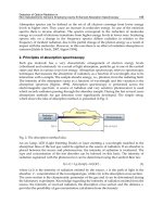
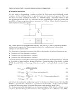
Fig. 1 Sampling spears
The spear is thrust into the powder with the inner chamber closed off, and when in position the outer tube is rotated to
allow powder to fall into the inner chamber. When the chamber is full, the inner tube is turned to the closed position and
the spear is withdrawn. Possible segregation throughout the bed may be investigated with type 3, an average value for the
length of the spear with type 2, and a spot sample with type 3. Frequently the spears are vibrated to facilitate filling, and
this can lead to an unrepresentative quantity of fines entering the sample volume. The sampling chambers also have a
tendency to jam if coarse particles are present, because they can get lodged between the inner and outer chambers.
Coning and Quartering. In industry it is common practice to sample small heaps by coning and quartering. The
powder is formed into a heap, which is first flattened at the top and then separated into four equal segments with a sharp-
edged board or shovel. The segments are drawn apart and, frequently, two opposite quadrants are recombined and the
operation is repeated until a small enough sample has been generated. This practice is based on the assumption that the
heap is symmetrical, and since this is rarely so, the withdrawn sample is usually nonrepresentative.
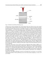
Sampling from Trucks or Wagons. Consignment sampling is carried out on a single consignment (e.g., a truck or
wagon load). In sampling from a truck or a wagon it is recommended that eight samples be extracted (Ref 1). No
increment should be taken at less than 12 in. below the surface; this avoids the surface layer, in which segregation can
have occurred due to vibration (Fig. 2). Care needs to be taken to prevent powder sliding down the slope created due to
removal of surface material.

Fig. 2 Sampling points for a wagon or a truck
Sampling Stored Free-Flowing Material. It is practically impossible to representatively sample stationary free-
flowing powder because of the severe segregation that has almost certainly occurred. There is only one sound piece of
advice to give regarding sampling such material: Don't! If there is no alternative, several samples should be taken and
analyzed separately so that an estimate can be made of the degree of segregation.
Sampling from Containers. Suppose an analysis is required from several tons of material that is available in bags or
small containers. Several of these containers should be selected systematically or, preferably, using a table of random
numbers. The recommended number of samples depends on the number of containers (Table 1). The whole of each bag
should then be sampled using a full stream or Vezin-type splitter so that the golden rules of sampling are obeyed. This is
the only way to obtain a representative sample from each bag. Where this is not possible a sampling thief may be used. It
is preferable to obtain a sample as the containers are being filled or emptied.
Table 1 Recommended number of containers to be sampled from a packaged lot

Number of

containers in lot

Number of containers to

be sampled
1-5
all
6-11
5
12-20
6
21-35
7
36-60
8
61-99
9
100-149
10
150-199
11
200-299
12
300-399
13
Note: For every additional 100 containers, one additional container should be sampled. Source: ISO 3954

Reference cited in this section
1.

"Sieve Analysis of Granular Mineral Surfacing for Asphalt Roofing and Shingles," D 451-
63, American
Society for Testing and Materials, 1963

Sampling and Classification of Powders
Terence Allen

Sampling Flowing Streams
Most powder systems are transported at some time during their manufacture as flowing streams: Hoppers are emptied by
screw or belt conveyors, powders are transferred to bagging operations by screw or pneumatic conveyors, and many
solids are transported through pipes. A general rule in all sampling is that whenever possible, the sample should be taken
while the powder is in motion. This is usually easy with continuous processes; with consignment sampling it may be
possible during filling and emptying of storage containers.
Sampling from a Conveyor Belt. When a sample is to be collected from a conveyor belt, the best position for
collecting the increments is where the material falls in a stream from the end of the belt. If access at such a point is not
possible, the sample must be collected from the belt. The whole of the powder on a short length of the belt must be
collected. The particles at the edge of the belt may not be the same as those at the center, and particles at the top of the
belt may not be the same as those at the bottom. If the belt can be stopped, the sample may be collected by inserting into
the stream a frame consisting of two parallel plates shaped to fit the belt; the whole of the material between the plates is
then swept out. A scoop can be used to scoop out an increment, but this operation can be hazardous if the belt is moving.
When sampling from a continuous stream, the sampling may be continuous or intermittent. In continuous sampling, a
portion of the flowing stream is split off and frequently further divided subsequently. In intermittent sampling, the whole
stream is taken for many short increments of time at fixed time intervals. These increments are usually compounded and
samples for analysis are taken from this gross sample. Continuous sampling is deprecated because if there is segregation
on the belt, the extracted sample may not be representative.
It is common practice, in sampling from a blender, to extract three samples: the first after the blender has been emptying
for a few minutes, the second when the blender is half empty, and the third when the blender is almost empty. Note that

blenders sometimes have a "heel" of unmixed material that is first out of the blender. Powder from the whole cross
section of the blender discharge steam should be collected for each sample. This practice should only be used after the
mixing efficiency of the blender has been established for each product by taking multiple samples and analyzing these
separately.
Point Samplers. Samples can be extracted from the product stream by projecting a sample tube, containing a nozzle or
orifice, into the flow. The particles impact the tube and fill the open cavity. The sampling head is out of the stream when
not sampling Snorkel-type samplers are available for vertical or inclined applications and can be preprogrammed for
sampling frequency. It is not possible to sample nonhomogeneous streams representatively with this type of device. With
the auger-type sampler, a slot inside the process stream is rotated to capture a cross section of the process stream, which is
then delivered into a sample container. This type of device does not collect a representative sample unless the stream is
homogeneous, and it has the added disadvantage that it obstructs flow.
Sampling from Falling Streams. In collecting from a falling stream of power, care should be taken to offset the
effects of segregation. Each increment should be obtained by collecting the whole of the stream for a short time. Care
must be taken in putting the sampler in and out of the stream. Figure 3 shows correct and incorrect ways of doing this.
Unless the time during which the receiver is stationary in its receiving position is long compared with the time taken to
insert and withdraw the sampler, the method shown in Fig. 3(a) will lead to an excess of coarse particles, because the
surface region of the stream, usually rich in coarse particles, is sampled for a longer time than the rest of the stream. The
method shown in Fig. 3(b) is not subject to this objection. If this method is not possible due to some obstruction, the ratio
of stationary to moving time for the receiver should be made as large as possible. In many cases it is not possible to
collect the whole of the stream as this would give too large an amount to be handled. The best procedure in this case is to
pass a sample collector of the form shown in Fig. 3(c) through the stream.

Fig. 3
Sampling from falling streams. (a) Bad sampling technique. (b) Good sampling technique. (c) Sampling
procedure to be adopted for high mass flow rate
The width of the receiver, b, should be chosen to give an acceptable weight of sample but must not be made so small that
the biggest particles have any difficulty in entering the receiver. Particles that strike the edges of the receiver are likely to
bounce out and not be collected, so that the effective width is (b-d), where d is the particle diameter. The effective width
is therefore greater for small particles than for large ones. To reduce this error to an acceptable level, the ratio of receiver
width to the diameter of the largest particle should be made as large as possible with a minimum value of 3:1. The depth,

a, must be great enough to ensure that the receiver is never full of powder. If the receiver fills before it finishes its
traverse through the powder, a wedge-shaped heap will form that is size selective. As more powder falls on top of the
heap, the fine particles will percolate through the surface and be retained, whereas the coarse particles will roll down the
sloping surface and be lost. The length of the receiver, c, should be sufficient to ensure that the full depth of the stream is
collected.
Stream Sampling Ladles. Powder may be manually withdrawn from a moving stream of powder using one of the
several commercially available ladles. These are suitable for occasional use, but automatic on-line stream sampling
samplers are preferred for frequent applications.
Traverse Cutters. With large tonnages, samples taken from conveyors can represent large quantities of material that
need to be further reduced. With the action shown in Fig. 4(a) and 4(b), uniform increments are withdrawn to give a
representative sample, but with the action shown in Fig. 4(c), a biased sample results if the inner and outer arcs of the
container are significantly different and the powder is segregated horizontally on the belt.

Fig. 4 Traversing cutters. (a) Straight path action, in line. (b) Cross line. (c) Oscillating or swinging arc path

Often, a traversing cutter is used as a primary sampler, and the extracted sample is further cut into a convenient quantity
by a secondary sampling device. The secondary sampler must also conform with the golden rules of sampling.
A traversing cutter is satisfactory for many applications, but it has limitations that restrict its use:
• Although a traversing cutter is comparatively readily designed into
a new plant, it is frequently difficult
and expensive to retrofit an existing plant because of the space requirements.
•
The quantity of sample obtained is proportional to product flow rate, and this can be inconvenient when
the plant flow rate is subject
to wide variations. On the other hand, where the daily average of a plant is
required, this is a necessary condition.
•
It is difficult to enclose the sampler to the extent required to prevent the escape of dust and fumes when
handling dusty powders.
Sampling Dusty Material. Figure 5 shows a sampler designed to sample a dusty material, sampling taking place only

on the return stroke. This is suitable provided that the trough extends the whole length of the stream and does not overfill.
The radial cutter or Vezin sampler shown in Fig. 6 is suitable for sample reduction. These samples vary in size from a 15
cm laboratory unit to a 152 cm commercial unit.

Fig. 5 Full-stream trough sampler

Fig. 6 Schematic of a primary and secondary syst
em based on Denver Equipment Company's type C and Vezin
samplers
Diverter Valve Sampler. The diverter valve shown in Fig. 7 is suitable for online intermittent sampling when there is
limited head room. It can also be operated manually.

Fig. 7 Diverter valve sampler
Sampling and Classification of Powders
Terence Allen

Sample Reduction
The gross sample is frequently too large to be handled easily and may have to be reduced to a more convenient weight.
Obviously, the method employed must conform with the two golden rules mentioned above. The amount of material to be
handled is usually small enough that getting it in motion poses no great difficulty. There is a natural tendency to remove
an aliquot with a scoop or spatula, and this must be avoided because it negates the effort involved in obtaining a
representative sample from the bulk. Placing the material in a container and shaking it to obtain a good mix prior to
extracting a scoop sample is not recommended.
To obtain the best results, the material should be made as homogeneous as possible by premixing. It is common practice
then to empty the material into a hopper, and this should be done with care. A homogeneous segregating powder will
segregate when fed to a hopper from a central inlet, because in essence it is being poured into a heap. In a core flow
hopper the central region (which, with improper feeding, will be rich in fines) empties first, followed by the material
nearer the walls, which has an excess of coarse particles. The walls of the hopper should have steep sides (at least 70°) to
ensure mass flow, and the hopper should be filled in such a way that size segregation does not occur. This can best be
done by moving the pour point about so that the surface of the powder is more or less horizontal. Several sample-dividing

devices are discussed briefly below.
Scoop sampling consists of plunging a scoop into the powder and removing a sample. This method is particularly
prone to error because the whole of the sample does not pass through the sampling device, and because the sample is
taken from the surface, where it may not be representative of the mass. For powder in a container, it is usual to shake the
sample prior to sampling in an attempt to achieve a good mix. However, the method of shaking can promote segregation.
Coning and quartering consists of pouring the powder into a heap and relying on its radial symmetry to give identical
samples when the heap is flattened and divided by a cross-shaped cutter. This method is no more accurate than scoop or
thief sampling, which are simpler to carry out, but gross errors are to be expected. Coning and quartering should never be
used with free-flowing powders.
Table Sampling. In a sampling table the material is fed to the top of an inclined plane in which there is a series of
holes. Prisms placed in the path of the stream break it into fractions. Some powder falls through the holes and is
discarded, while the powder remaining on the plane passes on to the next row of holes and prisms, and more is removed,
and so on. The powder reaching the bottom of the plane is the sample. The objection to this type of device is that it relies
on the initial feed being uniformly distributed, and on a complete mixing after each separation, and in general these
conditions are not achieved. As it relies on the removal of part of the stream sequentially, errors are compounded at each
separation, hence its accuracy is low.
Chute Splitting. The chute splitter consists of a V-shaped trough, along the bottom of which is a series of chutes that
alternately feed two trays placed on either side of the trough. The material is repeatedly halved until a sample of the
desired size is obtained. When carried out with great care this method can give satisfactory sample division, but it is
particularly prone to operator error, which is detectable by unequal splitting of the sample.
The above methods are all popular because the samplers contain no moving parts and are consequently inexpensive.
Rotatory Sample Divider. The rotary sample divider conforms to the golden rules of sampling. The preferred method
of using this device is to fill a mass flow hopper in such a way that segregation does not occur. The table is then set in
motion and the hopper outlet is opened so that the powder falls into the collecting boxes. The use of a vibratory feeder is
recommended to provide a constant flow rate. Several versions of this instrument are available, some of which were
designed for free-flowing powders, some for dusty powders, and some for cohesive powders. They handle quantities from
40 L down to a few grams.
Sampling and Classification of Powders
Terence Allen

Slurry Sampling
Slurry process streams vary in flow rate, solids concentration, and particle size distribution. Any sampling technique must
be able to cope with these variations without affecting the representativeness of the extracted sample. For batch sampling,
automatic devices are available where a sampling slot traverses intermittently across a free-falling slurry. Unfortunately, it
is difficult to improvise with this technique for continuous sampling, because such samplers introduce pulsating flow
conditions into the system.
Sampling and Classification of Powders
Terence Allen

Evaluation of Sampling
Experimental tests of sampling techniques are compared in Table 2 as an example. Binary mixtures of coarse and fine
sand (60:40 ratio) were examined (Ref 2) using various laboratory sampling techniques. In every case, 16 samples were
examined to give the standard deviations shown in column 2. It may be deduced that very little confidence can be placed
in the first three techniques and that the rotary sample divider is so superior to all other methods that it should be used
whenever possible.

Table 2 Reliability of selected sampling methods using a 60:40 sand mixture

Sampling technique Standard deviation, %

Coning and quartering

6.81
Scoop sampling
5.14
Table sampling
2.09
Chute slitting
1.01
Rotary sample dividing

0.146
Random variation
0.075


Reference cited in this section
2.

T. Allen, Particle Size Measurement, Chapman & Hall, 1997

Sampling and Classification of Powders
Terence Allen

Weight of Sample Required
Gross Sample. Analyses are carried out on a sample extracted from the bulk, which, irrespective of the precautions
taken, never represents the bulk exactly. The limiting (minimum) weight of the gross sample may be calculated, using a
simple formula to give an error within predesignated limits, provided that the weight of the gross sample is much smaller
than that of the bulk. The limiting weight is given by:


(Eq 1)
where M
s
is the limiting weight in grams, is the powder density in g · cm
-3
, is the variance of the tolerated sample
error, w
1
is the fractional mass of the coarsest size class being sampled, and is the arithmetic mean of the cubes of of

the extreme diameter in the size class in cubic centimeters. This equation is applicable when the coarsest class covers a
size range of not more than and and w
1
is less than 50% of the total sample. Table 3 gives sample values.
Table 3 Minimum sample mass required for sampling from a stream of powder

Upper sieve

size, m
Lower sieve

size, m
Mass % in

class (100w
1
)

Sample weight

required, g
600
420 0.1 37,500
420
300 2.5 474
300
212 19.2 14.9
212
150 35.6 1.32

Sample by Increments. For sampling a moving stream of powder, the gross sample is made up of increments. In this
case the minimum incremental weight is given by:


(Eq 2)
where M
i
is the average mass of the increment,
0
is the average rate of flow, w
0
is the cutter width for a traversing cutter,
and v
0
is the cutter velocity. If w
0
is too small, a biased sample deficient in coarse particles, results. For this reason w
0

should be at least 3d, where d is the diameter of the largest particle present in the bulk.
ISO 3081 suggests a minimum incremental mass based on the maximum particle size in millimeters. These values are
given in Table 4. Secondary samplers then reduce this to analytical quantities.
Table 4 Minimum incremental mass required for sampling from a stream of powder

Maximum particle size, mm

Minimum mass of increment, kg

250-150
40.0

150-100
20.0
100-50
12.0
50-20
4.0
20-10
0.8
10-0
0.3

Gy (Ref 3) proposed an equation relating the standard deviation, which he calls the fundamental error
F
, to the sample
size:


(Eq 3)
where W is the mass of the bulk; w = n is the mass of n increments, each of weight , that make up the sample; C is the
heterogeneity constant for the material being sampled; and d is the diameter of the coarsest element.
For the mining industry (Ref 3), Gy expressed the constant C in the form C = clfg where:


(Eq 4)
P is the investigated constant. is the true density of the material. l is the relative degree of homogeneity where for a
random mixture l = 1, and for a perfect mixture l = 0. f is a shape factor assumed to be equal to 0.5 for irregular particles
and 1 for regular particles. g is a measure of the width of the size distribution where g = 0.25 for a wide distribution and g
= 0.75 for a narrow distribution (i.e., d
max
<2d

min
).
For the pharmaceutical industry, Deleuil (Ref 4) suggested C = 0.1lc with the coarsest size being replaced by the 95%
size.
For W w, Eq 4 can be written:


(Eq 5)
where = t( F/P) and t = 3 (99.9% confidence level) for total quality.
• For d
95
= 100 m, = 1.5, P = 10
-3
(1000 ppm), = 0.2, l = 0.03 (random), and w = 1000 g.
• For d
95
= 100 m, = 1.5, P = 0.05, = 0.05, l = 1 (homogeneous), and w = 4 g.
• For d
95
= 20 m, = 1.5, P = 10
-4
(100 ppm), = 0.05, l = 0.03 (random), and w = 8000 g.


References cited in this section
3.

P. Gy, Sampling of Particulate Matter: Theory and Practice, Elsevier, Amsterdam, 1982
4.

M. Deleuil, Powder Technology and Pharmaceutical Processes, Handbook of Powder Technology,
Vol 9, D.
Chulia, M. Deleuil, and Y. Pourcelot, Ed., Elsevier, 1994
Sampling and Classification of Powders
Terence Allen

Powder Classification

Classification methods are used to obtain particular powder distributions or to exclude certain powder sizes from a
distribution. The general process for separating dispersed materials is known as "air classification" or "fluid
classification," where powder classification is based on the movement of the suspended particles at different points under
the influence of a force. The fluid is usually water or air, and the field force may involve gravity or centrifugal or coriolis
forces. The other forces of importance are the drag forces due to the relative flow between the particles and the flow
medium, and the inertia forces due to accelerated particle movement. The classification process is defined in terms of
sorting and sizing. The former includes processes such as froth flotation, where particles are separated on the basis of
chemical differences and particle density. The latter, which is covered here, is based only on differences in particle size.
In an ideal system the cut size is well defined and there are no coarse particles in the fine fraction, and vice versa. In
practice, however, there is always overlapping of sizes. The cut size may be predicted from theory, but this usually differs
from the actual cut size due to the difficulty of accurately predicting the flow pattern in the system. It is therefore
necessary to be able to predict the future performance of classifiers based on their past performance.
Sampling and Classification of Powders
Terence Allen

Basic Variables
Consider a single stage of a classifier where W, W
c
, and W
f
are the weights of the feed, coarse stream, and fine stream,
respectively; F(x), F

c
(x), and F
f
(x) are the cumulative fraction undersize of feed, coarse stream, and fine stream,
respectively; and x is particle size. Then:
W = W
c
+ W
f


(Eq 6)


(Eq 7)
The total fine efficiency may be defined as:


(Eq 8)
and the total coarse efficiency as:


(Eq 9)
so that E
f
+ E
c
= 1. The total efficiency has no value in determining the effectiveness of a classification process, because it
only defines how much of the feed ends up in one or other of the two outlet streams, not how much of the desired material
ends up in the correct outlet stream. To discover this, it is necessary to determine the grade efficiency, which is

independent of the feed, provided that the classifier is not overloaded:


(Eq 10a)


(Eq 10b)


(Eq 10c)


(Eq 10d)


(Eq 10e)
Similarly, the fine grade efficiency is defined as:


(Eq 11a)


(Eq 11b)
Hence, from Eq 7, 10, and 11:
G
c
(x) = 1 - G
f
(x)

(Eq 12)
These equations can be used to evaluate the grade efficiency of a classifier, provided that the total efficiency and the size
distribution of two of the streams are known. Results are usually plotted as grade efficiency curves of G
c
(x) or G
f
(x)
against x. The classifier separates on the basis of Stokes diameter, so it is preferable to carry out the size determinations
on the same basis.
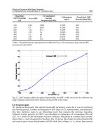
The grade efficiency curve is best determined by plotting F
c
(x) against F(x) and differentiating (Fig. 8b), because this
allows experimental errors to be smoothed out. The tangent at F
c
(x) = 100% in Fig. 8(b) has a slope of dF
c
(x)/dF(x) =
100/60; hence, E
c
= 60/100. Because this tangent merges with the curve at x = 58 m, all particles coarser than 58 m are
collected with the coarse fraction. Differentiating this curve at selected values of F(x) and multiplying by 60 gives G
c
(x),
the relevant diameters being determined from size distribution data. The 50% size on the grade efficiency curve is called
the equiprobable size because particles of this size have an equal chance of being in either the coarse or the fine stream.
Figure 8(a) shows how the feed is split between the coarse and fine fractions, i.e., F
f
(x) + F
c

(x) = F(x).

Fig. 8 Graphical determination of grade efficiency curve

The grade efficiency is often expressed as a single number. This number is known as the sharpness index, , and is a
measure of the slope of the grade efficiency curve:


(Eq 13)
where x
75
and x
25
are the particle sizes at which the grade efficiency is 75% and 25%, respectively. For perfect
classification = 1, while values above 3 are considered poor. Alternatively 10 90 has been used.
These ratios are not always adequate to define the sharpness of cut. In many cases it is important to keep the amount of
fines in the coarse or the amount of coarse in the fines as small as possible. For these cases a measure of the effectiveness
of a separation process is given by the following for the coarse yield:


(Eq 14a)


(Eq 14b)
Similarly, for the fine yield:


(Eq 15)
Sampling and Classification of Powders
Terence Allen

Systems for Powder Classification
Classifiers may be divided into two categories: counterflow equilibrium and crossflow separation.
Counterflow can occur in either a gravitational or centrifugal field. The field force and the drag force act in opposite
directions and particles leave the separation zone in one of two directions according to their size. At the "cut" size,
particles are acted on by two equal and opposite forces; hence, they stay in equilibrium in the separation zone. In
gravitational systems these particles remain in a state of suspension, while in a centrifugal field the equilibrium particles
revolve at a fixed radius, which is governed by the rate at which material is withdrawn from the system. They would
therefore accumulate to a very high concentration in a continuously operated classifier, if they were not distributed to the
coarse and fine fractions by a stochastic mixing process.
In a crossflow classifier, the feed material enters the flow medium at one point in the classification chamber, at an angle
to the direction of fluid flow, and is fanned out under the action of field, inertia, and drag forces. Particles of different
sizes describe different trajectories and so can be separated according to size.
Counterflow Equilibrium Classifiers in a Gravitational Field: Elutriators. Elutriation is a process of grading
particles by means of an upward current of fluid, usually air or water. The grading is carried out in one or a series of
containers, the bodies of which are cylindrical and the bases of which are inverted cones. The cut size is changed by
altering the volume flow rate and the cross-sectional areas of the elutriation chambers. The flow medium is usually air,
although water is used occasionally.
In air elutriators, air containing particles sweep up through the system at a preset flow rate. Particles with a settling
velocity lower than the air flow rate are carried out with the air stream, whereas larger particles are retained in the
elutriation chamber. The separation is very slow but can be speeded up by the use of zig-zag classifiers, which act as a
succession of elutriators in series.
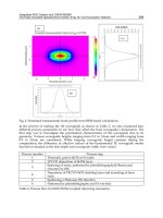
Zig-Zag Classifiers. Several versions of the zig-zag classifiers are available (Fig. 9). These may be categorized as
gravitational or centrifugal counterflow classifiers. A feed rating worm (b) feeds the unclassified material (c) into a
classifying chamber. Radially arranged blades on the outer face of the classifier rotor (d) speed the inflow of material up
to the peripheral velocity of the rotor suspending it, extra air being admitted through (e). The dust-air mixture is then
sucked in to the zig-zag-shaped rotor channels where classification takes place (Fig. 10). Fine material is sucked into the
classifier center (g), where it leaves via a cyclone. The coarse material (f) is expelled by centrifugal force. At the
periphery it is flushed by the incoming air before being discharged. Gravitational instruments operate in the 1 to 100 m
size range, centrifugal instruments from 0.1 to 6 m.

Fig. 9 The Alpine zig-zag centrifugal laboratory classifier


Fig. 10 Mode of action of a zig-
zag classifier. The small balls are the fine material; the large balls are the
coarse material. Bolts indicate the material guide motion
Cross-flow gravitational classification is performed with the Warmain Cyclosizer (Ref 5), which is a hydraulic
cyclone elutriator (Fig. 11). Using inverted cyclones as separators with water as the flow medium, samples of between 25
to 200 g are reduced to five fractions having cut sizes (for quartz) of 44, 33, 15, and 10 m. The cyclones are arranged in
series, and during a run the oversize for each cyclone is trapped and subjected to elutriating action for a fixed time period.
At the end of a run the trapped materials are extracted by opening the valves at the apex of each cyclone in turn, and after
decantation, the solids are recovered by filtration and evaporation.

Fig. 11 Principle of the Warmain Cyclosizer
Counterflow Centrifugal Classifiers. The Bahco Classifier is a centrifugal elutriator (Fig. 12). The sample is
introduced into a spiral air current created by a hollow disc rotating at 3500 rpm. Air and dust are drawn through the
cavity in a radially inward direction against centrifugal forces. Separation into different size fractions is made by altering
the air velocity, which is effected by changing the air inlet gap by the use of spacers. Instrument calibration is necessary.
For the sample, 5 to 10 g of powder are required, which can be graded in the size range 5 to 100 m.

Fig. 12 Simplified schematic diagram of the Bahco microparticle
classifier. 1, electric motor; 2, threaded
spindle; 3, symmetrical disk; 4, sifting chamber; 5, container; 6, housing; 7, top edge; 8, radial vanes; 9, feed
point; 10, feed hole; 11, rotor; 12, rotary duct; 13, feed slot; 14, fanwheel outlet
Crossflow Centrifugal Classifiers. The principle of a crossflow centrifugal laboratory classifier is illustrated in Fig.
13. A vaned rotor produces a centrifugal field, while at the same time air is drawn into the center of the rotor. All but
about 5% of the air intake, induced by a positive displacement pump downstream of the classifier, enters the classification
zone through a very narrow gap formed between the rotor and the stator. This leads to a very high turbulence in the
preclassification zone. The material enters the classifier through a venturi-type nozzle with the remaining 5% of air.

Between planes 1 and 2 the ratio of centrifugal force to drag force is kept very nearly constant by a diverging radial cross
section. This zone is the classification zone. The smaller particles are carried out through the middle and the larger ones
move toward the stator, where they undergo disaggregation until they reach the exit. The cut size of these machines
ranges from 0.5 to 50 m.

Fig. 13 A cross-flow centrifugal laboratory classifier
Crossflow Elbow Classifier. In the cross-flow air classifier (Fig. 14) the main air is introduced at a
1
and secondary air
at a
2
. Both streams are bent around a solid wall (b), and the resulting flow follows the bend without leaving the wall or
forming vortices. The so-called Coanda effect helps to maintain the flow around the bend for approximately 90°, and this
is enhanced by the application of suction.

Fig. 14 Principle of the cross-flow elbow classifier


Reference cited in this section
5.

D.F. Kelsall and J.C.H. McAdam, Trans. Inst. Chem Eng., Vol 41, 1963, p 84-94

Sampling and Classification of Powders
Terence Allen

Sieving Methods

Sieving methods are used to obtain particular powder distributions or to obtain narrow size ranges of a powder. Sieving is
a particularly useful procedure because particles are sorted into categories solely on the basis of size, independently of

other properties (density, surface, etc.). It can be used to classify dry or wet powders and generates narrowly classified
fractions. With micromesh sieves, near-monodisperse powders can be generated in the range of 1 to 10 m.
Sieving consists of placing a powder sample on a sieve containing openings of a fixed size and agitating the sieve in such
a way that particles that can pass through the openings do so. To speed up the analysis, several sieves are stacked on top
of each other, with the sieve containing the coarsest openings on top. This "nest" of sieves is vibrated until the residue on
each sieve contains particles that could pass through the upper sieve but not through the lower sieve.
A variety of sieve apertures are currently available, ranging in size from about 20 m to millimeters for woven wire
sieves, down to 5 m or less for electroformed sieves, and greater than 1 mm for punched plate sieves. Woven wire
sieves generally have pseudosquare apertures (i.e., the weaving process generates trapezoidal apertures in three
dimensions), but punched plate and electroformed sieves are available with round and rectangular apertures. A variety of
other shapes are also readily available.
Sieve analysis presents three major difficulties. With woven wire sieves the weaving process produces three-dimensional
apertures with considerable tolerances, particularly for fine-woven mesh (Ref 2). The mesh is easily damaged in use (Ref
3). The particles must be efficiently presented to the sieve apertures.
Fractionation by sieving is a function of two dimensions only, maximum breadth and maximum thickness, because unless
the particles are excessively elongated, the length does not affect the passage of particles through the sieve apertures (Fig.
15). Particles having two dimensions smaller than the openings will pass through when the sieve is vibrated, whereas
larger particles will be retained. The sieve size d
A
is defined, on the basis of woven wire sieves, as the minimum square
aperture through which a particle can pass.

Fig. 15 Sieved size of an irregularly shaped particle
The sieve surface consists of a go/no-go barrier: particles much smaller in size pass through rapidly, and larger particles
pass through more slowly. The apertures have a range of sizes, so the final particle that can pass through will pass through
the largest opening when its two smaller dimensions are in a preferred direction. Because this takes a very long time,
sieving is usually deemed complete when not more than 0.2% of the original weight of sample passes through in a 2 min
sieving operation (Ref 6).
Sieves are often referred to by their mesh size, which is the number of wires per linear inch. American Society for Testing
Materials standards range from 635 mesh (20 m) to 5 mesh (125 mm). The apertures for the 400 mesh are 37.5 m;

hence, the wire thickness is 26 m and the percentage open area is 35.
Sieve analyses can be highly reproducible even when different sets of sieves are used. Although most of the problems
associated with sieving have been known for many years and solutions have been proposed, reproducibility is rarely
achieved in practice due to failure to recognize these problems (Ref 7).

References cited in this section
2.

T. Allen, Particle Size Measurement, Chapman & Hall, 1997
3.

P. Gy, Sampling of Particulate Matter: Theory and Practice, Elsevier, Amsterdam, 1982
6.

"Methods for the Use of Fine-Mesh Sieves," S 1796, British Standard Specifications, 1952
7.

K. Leschonski, in Proc. Particle Size Analysis Conf., M.J. Groves, Ed., Heyden, London, 1977, p 205-217

Sampling and Classification of Powders
Terence Allen

Sieve Types
Woven-Wire and Punched Plate Sieves. Sieve cloth is woven from wire, and the cloth is soldered and clamped to
the bottom of cylindrical containers (Ref 8). Although the apertures are described as square, they deviate from this shape
due to the three-dimensional structure of the weave. Heavy-duty sieves are often made of perforated plate, giving rise to
circular holes (Ref 9). Various other shapes, such as slots for sieving fibers, are also available. Fine sieves are usually
woven with phosphor bronze wire, medium sieves with brass, and coarse sieves with mild steel. Special-purpose sieves
are also available in stainless steel, and the flour industry uses nylon or silk. A variety of electroformed sieves are also
available.

The cylindrical sieve cloth containers (sieves) are formed in such a way that they will stack, one on top of another, to give
a snug fit (Fig. 16).

Fig. 16 Stacked sieves on a shaker with rotary and tapping action

A variety of sieve aperture ranges are currently used, and these may be classified as coarse (4 to 100 mm), medium (0.2 to
4 mm), and fine (less than 0.2 mm). The fine range extends down to 20 m with woven wire mesh and to 5 m or less
with electroformed sieves.
Large-scale sieving machines, to take a charge of 50 to 100 kg, are needed for the coarse range. A wide range of
commercial sieve shakers are available for the medium range, and these usually classify the powder into five or six
fractions with a loading of 50 to 100 g. Special sieving techniques are used with the finer micromesh sieves.
Due to the method of manufacture, woven wire sieves have poor tolerances, particularly as the aperture size decreases.
Tolerances are improved and the lower size limit is extended with the electroformed micromesh sieves.
Electroformed Micromesh Sieves. Micro-mesh sieves (Ref 10), generated by a photoetching process, are available
in a wide range of sizes and aperture shapes.
Basically, the photoetching process is as follows. A fully degreased metal sheet is covered on both sides with a
photosensitive coating and the desired pattern is applied photographically to both sides of the sheet. Subsequently the
sheet is passed through an etching machine and the unexposed metal is etched away. Finally, the photosensitive coating is
removed. A supporting grid is made by printing a coarse line pattern on both sides of a sheet of copper foil coated with
photosensitive enamel. The foil is developed and the material between the lines is etched away. The mesh is drawn tautly
over the grid and nickel plated onto it. The precision of the method gives a tolerance of 2 m for apertures from 300 to
500 m reducing to 1 m for apertures from 5 to 106 m. For square mesh sieves the pattern is ruled onto a wax-coated
glass plate with up to 8000 lines per inch, with each line 0.0001 in. wide, and the grooves are etched and filled. The lower
limit for off-the-shelf sieves is about 5 m but apertures down to 1 m have been produced. Apertures are normally
square or round. The percentage of open area decreases with decreasing aperture size, ranging from 2.4% for 5 m
aperture sieves to 31.5% for 40 m aperture sieves. This leads to greatly extended sieving time when the smaller aperture
sieves are used.
Some round aperture sieves have apertures in the shape of truncated cones with the small circle uppermost. This reduces
blinding but also reduces the open area and therefore prolongs the sieving time. When sturdier thicker sieves are required,
they are subjected to further electrodeposition on both sides to produce biconical apertures.

The tolerances with micromesh sieves are much better than those for woven-wire sieves, the apertures being guaranteed
to ±2 m of nominal size except for the smaller-aperture sieves. Each type of sieve has advantages and disadvantages; for
example, sieves having a large percentage of open area are structurally weaker but measurement time is reduced.
Size and shape accuracy are improved by depositing successive layers of nickel and copper on a stainless steel plate,
followed by etching through a photolithographic mask additional layers of copper and nickel. The holes are filled with
dielectric, after which the additional nickel is removed down to the copper layer.
Dry sieving is often possible with the coarser micromesh sieves, and this may be speeded up, and the lower limit
extended, with air jet and sonic sifting. Agglomeration of the particles can sometimes be reduced by drying or adding
about 1% of a dispersant such as stearic acid or fumed silica. If this is unsuccessful, wet methods may have to be used.
Ultrasonics are frequently used as an aid to sieving or for cleaning blocked sieves, The delicate mesh can be ruptured
under these conditions, and this readily occurs at low frequencies. The rate of cavitation is less in hydrocarbons than in
alcohol and about six times greater in water than in alcohol. Saturating the alcohol with carbon dioxide reduces the rate.
An upper limit of 40 kHz and a power level of 40 W is recommended. Still higher frequencies reduce the amount of
erosion. ASTM E 161-70 recommends cleaning sieves, 15 to 20 s at a time, with a low-power 40 kHz ultrasonic bath
containing an equivolume mixture of isopropyl or ethyl alcohol and water with the sieve in a vertical position.
Standard Sieves. The United States Standard Sieve Series described by ASTM (Ref 8) ranges from 20 m to 5 in.
According to ASTM, the nominal 75 m sieve has a median aperture size in the range of 70 to 80 m, and not more 5%
of the apertures shall fall in the intermediate to maximum size range of 91 to 103 m. This implies that there is a
probability of having a 103 m aperture in a nominal 75 m sieve. It is clear that oversize apertures are more undesirable
than undersize ones, because the latter are merely ineffective while the former permit the passage of oversize particles.
The relative tolerance increases with decreasing nominal size, leading to poor reproducibility when analyses are carried
out using different nests of uncalibrated sieves. Electroformed sieves with square or round apertures and tolerances of ±2
m are also available.
Complete instructions and procedures on the use and calibration of testing sieves are contained in Ref 11. This publication
also contains a list of all published ASTM standards on sieve analysis procedures for specific materials or industries.
Standard frames are available with nominal diameters of 3, 6, 8, 10, or 12 in. Nonstandard frames are also available.
Most test sieves are certified and manufactured to ISO 9002 standards. Woven-wire sieves, having apertures ranging from
20 m to 125 mm, are readily available in 100, 200, 300, and 450 mm diameters as well as 3, 8, 12, and 18 in. diameters.
Microplate sieves are available in 100 and 200 mm diameters with round or square apertures ranging from 1 to 125 mm.
Micromesh electroformed sieves are available in 3, 8, and 12 in. diameter frames, as well as custom-made sizes. Sieves

have apertures ranging from 5 to 500 m, and other apertures are available. Etched sieves have round apertures ranging
from 500 to 1200 m.

References cited in this section
8. "Standard Specification for Wire-Cloth Sieves for Testing Purposes," E 11-
87, American Society for
Testing and Materials
9. "Standard Specifications for Perforated Plate Sieves for Testing Purposes," E 323-
80, American Society for
Testing and Materials, reapproved 1990
10.

"Standard Specification for Precision Electroformed Sieves (Square Aperture)," E 161-
87, American
Society for Testing and Materials, reapproved 1992
11.

Manual on Testing Sieving Methods, STP 447B, American Society for Testing and Materials
Sampling and Classification of Powders
Terence Allen

Process Variables
End Point of the Sieving Process. The nominal wire thickness for a 75 m sieve is 52 m. Hence, at the
commencement of a sieving operation, the nominal open area comprises 35% of the total area [i.e., (75/127)
2
], with
apertures ranging in size from 42 to 108 m (Fig. 17). As sieving progresses, the number of particles that can pass
through the smaller aperture decreases, as well as the percentage of available open area. At the same time the effective
sieve size increases, rising, in the example given above, to 84 m, then to 94 m, and eventually to the largest aperture in
the sieve cloth. Thus, the mechanism of sieving can be divided into two regions with a transition region in between: an

initial region that relates to the passage of particles much finer than the mesh openings, and a second region that relates to
the passage of near-mesh particles (Fig. 18). Near-mesh particles are defined as particles that will pass through the sieve
openings in only a limited number of ways, and the ultimate particle is the one that will pass only through the largest
aperture in only one orientation.

Fig. 17 Effective aperture width distribution with increasing sieving time

Fig. 18 The rate at which particles pass through a sieve

The end point of sieving should be selected at the beginning of region 2. This can be done by plotting the time-weight
curve on log-probability paper and selecting the end point. It is difficult to do this in practice, and an alternative procedure
is to use a log-log plot and define the end point as the intersection of the extrapolation for the two regions (Fig. 18).
Using the conventional rate test, the sieving operation is terminated sometime during region 2. The true end point, when
every particle capable of passing through a sieve has done so, is not reached unless the sieving time is unduly protracted.
Near-mesh particles are defined as particles that pass through the sieve openings in only a limited number of ways relative
to the many possible orientations with respect to the sieve surface. The passage of such particles is a statistical process;
that is, there is always an element of chance as to whether a particular particle will or will not pass through the sieve. In
the limit, the sieving process is controlled by the largest aperture through which the ultimate particle will pass in only one
particular orientation. In practice there is no end point to a sieving operation, so this is defined in an arbitrary manner.
The rate method is fundamentally more accurate than the time method, but it is more tedious to apply in practice, and for
most routine purposes a specified sieving time is adequate.
Conventional dry sieving is not recommended for brittle material because attrition takes place and an end point is difficult
to define. The rate of passage of particles may fail to decrease with sieving time due to particle attrition, particle
deagglomeration, or a damaged sieve.
Calibration of Sieves. It is not widely realized that analyses of the same sample of material by different sieves of the
same nominal aperture size are subject to discrepancies, which may be considerable. These discrepancies may be due to
nonrepresentative samples, differences in the amount of time the material is sieved, operator errors, humidity, different
sieving actions, and differences in the sieves themselves.
Ideally, sieves should have apertures of identical shape and size. However, due to the methods of fabrication, woven-wire
sieves have a range of aperture sizes and weaving gives a three dimensional effect. Fairly wide tolerances are accepted

and specified in standards, but even these are sometimes exceeded in practice. In order to obtain agreement between
different sets of sieves it is therefore necessary to calibrate them and thenceforth to monitor them to detect signs of wear.
One way of standardizing a single set of sieves is to analyze the products of comminution. It is known that the products
are usually log-normally distributed; hence, if the distribution is plotted on a log-probability paper a straight line should
result. The experimental data are fitted to the best straight line by converting the nominal sieve aperture to an effective
sieve aperture.
The traditional method of determining the median and spread of aperture sizes for a woven-wire sieve is to size a
randomly selected set of apertures using a microscope. Due to the method of manufacture the measurements for the warp
and weft will tend to differ. The limiting size may also be determined by using spherical particles. These are fed onto the
sieve, the sieve is shaken, and the excess is removed. Many spheres will have jammed into the sieve cloth and may be
removed for microscopic examination.
Sieves may be monitored using glass beads, available from the National Bureau of Standards, every few months to find
out whether the sieve apertures are deteriorating or enlarging. The whole sample is placed on the sieves and shaken in the
manner in which tests will be made on test samples. The percentage retained on each sieve is determined and the effective
opening on each sieve is determined from calibration data supplied with the bead set. Standard polystyrene spheres are
also available for calibration purposes from laboratory supplies (such as Gilson and Duke Standards).
Sieves may also be calibrated by a counting and weighing technique applied to the fraction of particles passing the sieve
immediately prior to the end of an analysis. These will have a very narrow size range and the average particle size may be
taken as the cut size of the sieve. A minimum number (n) of particles need to be weighed to obtain accurate volume
diameters (d
v
). Let this weight be m and the particle density be , then:


(Eq 16)
Particles larger than 250 m can be easily counted by hand and, if weighed in batches of 100, d
v
is found to be
reproducible to three significant figures. For particles between 100 and 250 m, it is necessary to count in batches of
1000 using a magnifier. For sizes smaller than this the Coulter principle can be used to obtain the number concentration in

a known suspension. Sieve analyses are then plotted against volume diameter in preference to the nominal sieve diameter.
The method is tedious and time consuming, and the Community Bureau of Reference in Brussels has prepared quartz
samples by this method for use as calibration material. The quartz is fed to a stack of sieves, and the analytical cut size is
read off the cumulative distribution curve of the calibration material.
Sieving Errors. Hand sieving is the reference technique by which other sieving techniques should be judged. For
instance, the French standard NFX 11-57 states: "If sieving machines are used, they must be built and used in such a way
that the sieve analysis must, within the agreed tolerances, agree with the analysis obtained by hand sieving."
The apertures of a sieve may be regarded as a series of gages that reject or pass particles as they are presented at the
aperture. The probability that a particle will present itself to an aperture depends on:
• The particle size distribution of the powder. The presence of a large fraction of near-
mesh particles
reduces the sieving efficiency. An excess of fines has the same effect.
• The number of particles on the sieve (load).
The smaller the sieve loading, the more rapid the analysis.
Too low a load, however, leads to errors in weighing and unacceptable percentage losses.
• The physical properties of the particles. These include adhesion and other surface phenomena.
• The method of shaking the sieve.
Sieve motion should minimize the risk of aperture blockage and
preferably include a jolting action to remove particles that have wedged in the sieve mesh.
• Particle shape. Elongated particles sieve more slowly than compact particles.
• The geometry of the sieving surface
(e.g., the fractional open area). Whether or not the particle will pass
the sieve when it is presented at the sieving surface will depend on its
dimensions and the angle at
which it is presented.
The size distribution given by the sieving operation also depends on:
• Duration of sieving
• Variation of sieve aperture
• Wear
• Errors of observation and experiment

• Errors of sampling
• Effect of different equipment and operation
It is evident that a reduction in sieve loading is more effective than prolonging the sieving. It is therefore recommended
that the sample should be as small as is compatible with convenient handling. Although differences between analyses are
inevitable, standardization of procedure more than doubles the reproducibility of a sieving operation. Sieve calibration
increases this even further.
Sampling and Classification of Powders
Terence Allen

Methods of Sieving
Large-scale sieving machines, requiring a charge of 50 to 100 kg of powder, are used for the coarsest size range. A range
of commercial sieve shakers are available for medium-sized-aperture sieves, and they usually classify the powder into
five or six fractions, with a charge of 50 to 100 g.
Dry sieving is used for coarse separation, but other procedures are necessary as the powder becomes finer and more
cohesive. Machine sieving is performed by stacking sieves in ascending order of aperture size and placing the powder on
the top sieve. The most aggressive action is performed with Pascal Inclyno and Tyler Ro-tap sieves, which combine
gyrating and jolting movements, although a simple vibratory action may be suitable in many cases. Automatic machines
use an air jet to clear the sieves or ultrasonics to effect passage through the apertures. The sonic sifter combines two
actions, a vertically oscillating column of air and a repetitive mechanical pulse. Wet sieving is frequently used with
cohesive powders.
Amount of Sample Required. In determining the amount of sample to be used, it is necessary to consider the type of
material, its sievability, and the range of sizes present. Two opposing criteria must be met: it is necessary to use sufficient
material for accurate weighing and a small enough sample that the sieving operation is completed in a reasonable time.