Fourier Transform Pairs

209
CHAPTER
11
Fourier Transform Pairs
For every time domain waveform there is a corresponding frequency domain waveform, and vice
versa. For example, a rectangular pulse in the time domain coincides with a sinc function [i.e.,
sin(x)/x] in the frequency domain. Duality provides that the reverse is also true; a rectangular
pulse in the frequency domain matches a sinc function in the time domain. Waveforms that
correspond to each other in this manner are called Fourier transform pairs. Several common
pairs are presented in this chapter.
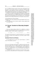
Delta Function Pairs
For discrete signals, the delta function is a simple waveform, and has an
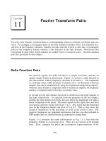
equally simple Fourier transform pair. Figure 11-1a shows a delta function in
the time domain, with its frequency spectrum in (b) and (c). The magnitude
is a constant value, while the phase is entirely zero. As discussed in the last
chapter, this can be understood by using the expansion/compression property.
When the time domain is compressed until it becomes an impulse, the frequency
domain is expanded until it becomes a constant value.
In (d) and (g), the time domain waveform is shifted four and eight samples to
the right, respectively. As expected from the properties in the last chapter,
shifting the time domain waveform does not affect the magnitude, but adds a
linear component to the phase. The phase signals in this figure have not been
unwrapped, and thus extend only from -B to B. Also notice that the horizontal
axes in the frequency domain run from -0.5 to 0.5. That is, they show the
negative frequencies in the spectrum, as well as the positive ones. The
negative frequencies are redundant information, but they are often included in
DSP graphs and you should become accustomed to seeing them.
Figure 11-2 presents the same information as Fig. 11-1, but with the
frequency domain in rectangular form. There are two lessons to be learned
here. First, compare the polar and rectangular representations of the
The Scientist and Engineer's Guide to Digital Signal Processing210

Sample number
0 16 32 48 64
-1
0
1
2
63
d. Impulse at x[4]
Sample number
0 16 32 48 64
-1
0
1
2
63
a. Impulse at x[0]
Frequency
-0.5 0 0.5
-2
-1
0
1
2
e. Magnitude
Frequency
-0.5 0 0.5
-6
-4
-2
0

2
4
6
f. Phase
Frequency
-0.5 0 0.5
-2
-1
0
1
2
h. Magnitude
Frequency
-0.5 0 0.5
-6
-4
-2
0
2
4
6
i. Phase
Frequency
-0.5 0 0.5
-2
-1
0
1
2
b. Magnitude

Frequency
-0.5 0 0.5
-6
-4
-2
0
2
4
6
c. Phase
Sample number
0 16 32 48 64
-1
0
1
2
63
g. Impulse at x[8]
Frequency DomainTime Domain
Amplitude
Phase (radians)
Amplitude
Amplitude
Phase (radians)
Amplitude
Amplitude
Phase (radians)
Amplitude
FIGURE 11-1
Delta function pairs in polar form. An impulse in the time domain corresponds to a

constant magnitude and a linear phase in the frequency domain.
frequency domains. As is usually the case, the polar form is much easier to
understand; the magnitude is nothing more than a constant, while the phase is
a straight line. In comparison, the real and imaginary parts are sinusoidal
oscillations that are difficult to attach a meaning to.
The second interesting feature in Fig. 11-2 is the duality of the DFT. In the
conventional view, each sample in the DFT's frequency domain corresponds
to a sinusoid in the time domain. However, the reverse of this is also true,
each sample in the time domain corresponds to sinusoids in the frequency
domain. Including the negative frequencies in these graphs allows the
duality property to be more symmetrical. For instance, Figs. (d), (e), and
Chapter 11- Fourier Transform Pairs 211
Sample number
0 16 32 48 64
-1
0
1
2
63
d. Impulse at x[4]
Sample number
0 16 32 48 64
-1
0
1
2
63
a. Impulse at x[0]
Frequency
-0.5 0 0.5

-2
-1
0
1
2
e. Real Part
Frequency
-0.5 0 0.5
-2
-1
0
1
2
f. Imaginary part
Frequency
-0.5 0 0.5
-2
-1
0
1
2
h. Real Part
Frequency
-0.5 0 0.5
-2
-1
0
1
2
i. Imaginary part

Frequency
-0.5 0 0.5
-2
-1
0
1
2
b. Real Part
Frequency
-0.5 0 0.5
-2
-1
0
1
2
c. Imaginary part
Sample number
0 16 32 48 64
-1
0
1
2
63
g. Impulse at x[8]
Frequency DomainTime Domain
Amplitude
Amplitude
Amplitude
Amplitude
Amplitude

Amplitude
Amplitude
Amplitude
Amplitude
FIGURE 11-2
Delta function pairs in rectangular form. Each sample in the time domain results in a cosine wave in the real part,
and a negative sine wave in the imaginary part of the frequency domain.
(f) show that an impulse at sample number four in the time domain results in
four cycles of a cosine wave in the real part of the frequency spectrum, and
four cycles of a negative sine wave in the imaginary part. As you recall, an
impulse at sample number four in the real part of the frequency spectrum
results in four cycles of a cosine wave in the time domain. Likewise, an
impulse at sample number four in the imaginary part of the frequency spectrum
results in four cycles of a negative sine wave being added to the time domain
wave.
As mentioned in Chapter 8, this can be used as another way to calculate the
DFT (besides correlating the time domain with sinusoids). Each sample in the
time domain results in a cosine wave being added to the real part of the
The Scientist and Engineer's Guide to Digital Signal Processing212
EQUATION 11-1
DFT spectrum of a rectangular pulse. In this
equation, N is the number of points in the
time domain signal, all of which have a value
of zero, except M adjacent points that have a
value of one. The frequency spectrum is
contained in , where k runs from 0 to
X[k]
N/2. To avoid the division by zero, use
. The sine function uses radians,
X[0] ' M

not degrees. This equation takes into
account that the signal is aliased.
Mag X [k] '
/
0
0
0
sin(BkM/N )
sin(Bk/N )
/
0
0
0
frequency domain, and a negative sine wave being added to the imaginary part.
The amplitude of each sinusoid is given by the amplitude of the time domain
sample. The frequency of each sinusoid is provided by the sample number of
the time domain point. The algorithm involves: (1) stepping through each time
domain sample, (2) calculating the sine and cosine waves that correspond to
each sample, and (3) adding up all of the contributing sinusoids. The resulting
program is nearly identical to the correlation method (Table 8-2), except that
the outer and inner loops are exchanged.
The Sinc Function
Figure 11-4 illustrates a common transform pair: the rectangular pulse and the
sinc function (pronounced “sink”). The sinc function is defined as:
, however, it is common to see the vague statement: "thesinc(a) ' sin(Ba)/(Ba)
sinc function is of the general form: ." In other words, the sinc is a sinesin(x)/x
wave that decays in amplitude as 1/x. In (a), the rectangular pulse is
symmetrically centered on sample zero, making one-half of the pulse on the
right of the graph and the other one-half on the left. This appears to the DFT
as a single pulse because of the time domain periodicity. The DFT of this

signal is shown in (b) and (c), with the unwrapped version in (d) and (e).

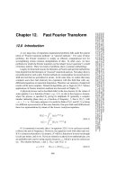
First look at the unwrapped spectrum, (d) and (e). The unwrapped
magnitude is an oscillation that decreases in amplitude with increasing
frequency. The phase is composed of all zeros, as you should expect for
a time domain signal that is symmetrical around sample number zero. We
are using the term unwrapped magnitude to indicate that it can have both
positive and negative values. By definition, the magnitude must always be
positive. This is shown in (b) and (c) where the magnitude is made all
positive by introducing a phase shift of B at all frequencies where the
unwrapped magnitude is negative in (d).
In (f), the signal is shifted so that it appears as one contiguous pulse, but is no
longer centered on sample number zero. While this doesn't change the
magnitude of the frequency domain, it does add a linear component to the
phase, making it a jumbled mess. What does the frequency spectrum look like
as real and imaginary parts ? Too confusing to even worry about.
An N point time domain signal that contains a unity amplitude rectangular pulse
M points wide, has a DFT frequency spectrum given by:
Chapter 11- Fourier Transform Pairs 213
Frequency
0 0.1 0.2 0.3 0.4 0.5
-6
-4
-2
0
2
4
6
e. Phase
Frequency

0 0.1 0.2 0.3 0.4 0.5
-5
0
5
10
15
20
g. Magnitude
Frequency
0 0.1 0.2 0.3 0.4 0.5
-6
-4
-2
0
2
4
6
h. Phase
Frequency
0 0.1 0.2 0.3 0.4 0.5
-5
0
5
10
15
20
b. Magnitude
Frequency
0 0.1 0.2 0.3 0.4 0.5
-6

-4
-2
0
2
4
6
c. Phase
Sample number
0 32 64 96 128
-1
0
1
2
127
f. Rectangular pulse
Frequency DomainTime Domain
or
Amplitude
Phase (radians)
Amplitude
Phase (radians)
Amplitude
Phase (radians)
Amplitude
FIGURE 11-3
DFT of a rectangular pulse. A rectangular pulse in one domain corresponds to a sinc
function in the other domain.
Sample number
0 32 64 96 128
-1

0
1
2
127
a. Rectangular pulse
Frequency
0 0.1 0.2 0.3 0.4 0.5
-5
0
5
10
15
20
d. Unwrapped Magnitude
Amplitude
EQUATION 11-2
Equation 11-1 rewritten in terms of the
sampling frequency. The parameter, , isf
the fraction of the sampling rate, running
continiously from 0 to 0.5. To avoid the
division by zero, use .Mag X(0) 'M
Mag X (f ) '
/
0
0
0
sin(B f M )
sin(B f )
/
0

0
0
Alternatively, the DTFT can be used to express the frequency spectrum as a
fraction of the sampling rate, f:
In other words, Eq. 11-1 provides samples in the frequency spectrum,N/2 %1
while Eq. 11-2 provides the continuous curve that the samples lie on. These
The Scientist and Engineer's Guide to Digital Signal Processing214
x
0.0 0.2 0.4 0.6 0.8 1.0 1.2 1.4 1.6
0
0.2
0.4
0.6
0.8
1
1.2
1.4
1.6
y(x) = x
y(x) = sin(x)
FIGURE 11-4
Comparing x and sin(x). The functions: ,y(x) ' x
and are similar for small values of x,
y(x) ' sin(x)
and only differ by about 36% at 1.57 (B/2). This
describes how aliasing distorts the frequency
spectrum of the rectangular pulse from a pure
sinc function.
y(x)
equations only provide the magnitude. The phase is determined solely by the

left-right positioning of the time domain waveform, as discussed in the last
chapter.
Notice in Fig. 11-3b that the amplitude of the oscillation does not decay to
zero before a frequency of 0.5 is reached. As you should suspect, the
waveform continues into the next period where it is aliased. This changes
the shape of the frequency domain, an effect that is included in Eqs. 11-1
and 11-2.
It is often important to understand what the frequency spectrum looks like when
aliasing isn't present. This is because discrete signals are often used to
represent or model continuous signals, and continuous signals don't alias. To
remove the aliasing in Eqs. 11-1 and 11-2, change the denominators from
respectively. Figure 11-4 showssin (B k / N ) to B k / N and from sin (B f ) to B f,
the significance of this. The quantity can only run from 0 to 1.5708, since B f f
can only run from 0 to 0.5. Over this range there isn't much difference
between and . At zero frequency they have the same value, andsin(B f ) B f
at a frequency of 0.5 there is only about a 36% difference. Without
aliasing, the curve in Fig. 11-3b would show a slightly lower amplitude
near the right side of the graph, and no change near the left side.

When the frequency spectrum of the rectangular pulse is not aliased
(because the time domain signal is continuous, or because you are ignoring
the aliasing), it is of the general form: , i.e., a sinc function. Forsin(x)/x
continuous signals, the rectangular pulse and the sinc function are Fourier
transform pairs. For discrete signals this is only an approximation, with the
error being due to aliasing.
The sinc function has an annoying problem at , where becomesx ' 0 sin(x)/x
zero divided by zero. This is not a difficult mathematical problem; as x
becomes very small, approaches the value of x (see Fig. 11-4).sin(x)