Applied Structural and Mechanical Vibrations 2009 Part 8 pdf
Bạn đang xem bản rút gọn của tài liệu. Xem và tải ngay bản đầy đủ của tài liệu tại đây (554.16 KB, 47 trang )
8.2.1 which are specified at a given time (usually t=0)—must be satisfied
at all times. Let us suppose that our string is attached to a rigid support
at x=0 and extends indefinitely in the positive x-direction (semi-infinite
string). This is probably the simplest type of boundary condition and it
is not difficult to see that such a ‘fixed-end’ situation mathematically
translates into
(8.23)
for all values of t: a condition which must be imposed on the general solution
f(x–ct)+g(x+ct). The final result is that the incoming wave g(x+ct) is reflected
at the boundary and produces an outgoing wave –g(x–ct) which is an exact
replica of the original wave except for being upside down and travelling in
the opposite direction. The fact that the original waveform has been reversed
is characteristic of the fixed boundary.
Another simple boundary condition is the so-called free end which can be
achieved, for example, when the end of the string is attached to a slip ring
of negligible mass m which, in turn, slides along a frictionless vertical post
(for a string this situation is quite artificial, but it is very important in many
other cases). In physical terms, we can write Newton’s second law stating
that the net transverse force F
y
(0, t) (due to the string) acting on the ring is
equal to Since and m is negligible, the free-
end condition is specified by
(8.24)
which asserts that the slope of string at the free end must be zero at all times.
By enforcing the condition (8.24) on the general d’Alembert solution, it is
now easy to show that the only difference between the original and the
reflected wave is that they travel in opposite directions: that is, the reflected
wave has not been inverted as in the fixed-end case. Note that, as expected,
in both cases—fixed and free end—the incoming and outgoing waves carry
the same amount of energy because neither boundary conditions allow the
string to do any work on the support. Other end conditions can be specified,
for example, corresponding to an attached end mass, a spring or a dashpot
or a combination thereof.
Mathematically, all these conditions can be analysed by equating the
vertical component of the string tension to the forces on these elements. For
instance, if the string has a non-negligible mass m attached at x=0, the
boundary condition reads
(8.25)
Copyright © 2003 Taylor & Francis Group LLC
or, say, for a spring with elastic constant k
0
(8.26)
Enforcing such boundary conditions on the general d’Alembert solution
makes the problem somewhat more complicated. However, on physical
grounds, we can infer that the incident wave undergoes considerable distortion
during the reflection process. More frequently, the reflection characteristics
of boundaries are analysed by considering the incident wave as pure harmonic,
thus obtaining a frequency-dependent relationship for the amplitude and
phase of the reflected wave.
8.3 Free vibrations of a finite string: standing waves and
normal modes
Consider now a string of finite length that extends from x=0 to x=L, is fixed
at both ends and is subjected to an initial disturbance somewhere along its
length. When the string is released, waves will propagate both toward the
left and toward the right end. At the boundaries, these waves will be reflected
back into the domain [0, L] and this process, if no energy dissipation occurs,
will continually repeat itself. In principle, a description of the motion of the
string in terms of travelling waves is still possible, but it is not the most
helpful. In this circumstance it is more convenient to study standing waves,
whose physical meaning can be shown by considering, for example, two
sinusoidal waves of equal amplitude travelling in opposite directions, i.e. the
waveform
(8.27a)
which, by means of familiar trigonometric identities, can be written as
(8.27b)
Two interesting characteristics of the waveform (8.27b) need to be pointed
out:
1. All points x
j
of the string for which sin(kx
j
)=0 do not move at all times,
i.e. y(x
j
, t)=0 for every t. These points are called nodes of the standing
wave and in terms of the waveform (8.27a), we can say that whenever
the crest of one travelling wave component arrives there, it is always
cancelled out by a trough of the other travelling wave.
Copyright © 2003 Taylor & Francis Group LLC
2. At some specified instants of time that satisfy all points x of the
string for which reach simultaneously the zero position and their
velocity has its greatest value. At other instants of time, when
all the above points reach simultaneously their individual maximum
amplitude value A sin(kx), and precisely at these times their velocity is zero.
Among these points, the ones for which sin(kx)=1 are alternatively crests
and troughs of the standing waveform and are called antinodes.
In order to progress further along this line of reasoning, we must investigate
the possibility of motions satisfying the wave equation in which all parts of
the string oscillate in phase with simple harmonic motion of the same
frequency. From the discussions of previous chapters, we recognize this
statement as the definition of normal modes.
The mathematical form of eq (8.27b) suggests that the widely adopted
approach of separation of variables can be used in order to find standing-
wave, or normal-mode, solutions of the one-dimensional wave equation.
So, let us assume that a solution exists in the form y(x, t)=u(x)z(t), where
u is a function of x alone and z is a function of t alone. On substituting this
solution in the wave equation we arrive at
which requires that a function of x be equal to a function of t for all x and
t. This is possible only if both sides of the equation are equal to the same
constant (the separation constant), which we call –
ω
2
. Thus
(8.28)
The resulting solution for y(x, t) is then
(8.29)
where and it is easy to verify that the product (8.29) results in a
series of terms of the form (8.27b). The time dependent part of the solution
represents a simple harmonic motion at the frequency
ω
, whereas for the
space dependent part we must require that
(8.30)
Copyright © 2003 Taylor & Francis Group LLC
because we assumed the string fixed at both ends. Imposing the boundary
conditions (8.30) poses a serious limitation to the possible harmonic motions
because we get A=0 and the frequency equation
(8.31)
which implies (n integer) and is satisfied only by those values of
frequency
ω
n
for which
(8.32)
These are the natural frequencies or eigenvalues of our system (the flexible string
of length L with fixed ends) and, as for the MDOF case, represent the frequencies
at which the system is capable of undergoing harmonic motion. Qualitatively,
an educated guess about the effect of boundary conditions could have led us to
argue that, when both ends of the string are fixed, only those wavelengths for
which the ‘matching condition’ (where n is an integer) applies can
satisfy the requirements of no motion at x=0 and x=L. This is indeed the case
and the allowed wavelengths satisfy etc.
The first four patterns of motion (eigenfunctions) are shown in Fig 8.2:
the motion for n=1, 3, 5,…result in symmetrical (with respect to the point
x=L/2) modes, while antisymmetrical modes are obtained for n=2, 4, 6,…
So, for a given value of n, we can write the solution as
(8.33)
where, for convenience, the constant of the space part has been absorbed in
the constants A
n
and B
n
. Then, given the linearity of the wave equation, the
general solution is obtained by the superposition of modes:
(8.34)
where the (infinite) sets of constants A
n
and B
n
represent the amplitudes of the
standing waves of frequency
ω
n
. The latter quantities, in turn, are related to the
allowed wavenumbers by the equation On physical grounds, since we
observed that there is no motion at the nodes and hence no energy flow between
neighbouring parts of the string, one could ask at this point how a standing
wave gets established and how it is maintained. To answer this question we
must remember that a standing wave represents a steady-state situation; during
the previous transient state (which, broadly speaking, we may call the ‘travelling
wave era’) the nodes move and allow the transmission of energy along the string.
Moreover, it should also be noted that nodes are not perfect in real strings
where friction is present; they are only points of minimum amplitude of vibration.
Copyright © 2003 Taylor & Francis Group LLC
Fig. 8.2 Vibration of a string with fixed ends: (c) third and (d) fourth modes.
which we recognize as Fourier series with coefficients A
n
and
ω
n
B
n
,
respectively. Following the standard methods of Fourier analysis, we multiply
both sides of eqs (8.35) by sin k
m
x and integrate over the interval [0, L] in
order to obtain, by virtue of
(8.36)
Copyright © 2003 Taylor & Francis Group LLC
the expressions
(8.37)
which establish the motion of our system. Note that eq (8.34) emphasizes
the fact that the string is a system with an infinite number of degrees of
freedom, where, in the normal mode representation, each mode represents a
single degree of freedom; furthermore, from the discussion above it is clear
that the boundary conditions determine the mode shapes and the natural
frequencies, while the initial conditions determine the contribution of each
mode to the total response (or, in other words, the contribution of each
mode to the total response depends on how the system has been started into
motion). If, for example, we set the string into motion by pulling it aside at
its centre and then letting it go, the ensuing free motion will comprise only
the odd (symmetrical) modes; even modes, which have a node at the centre,
will not contribute to the motion.
A final important result must be pointed out: when the motion is written
as the summation of modes (8.34), the total energy E of the string—i.e. the
integral of the energy density
over the length of the string—is given by
(8.38)
where it is evident that each mode contributes independently to the total
energy, without any interaction with other modes (recall Parseval’s theorem
stated in Chapter 2). The explicit calculation of (8.38), which exploits the
relation (8.36) together with its cosine counterpart
(8.39)
is left to the reader.
Copyright © 2003 Taylor & Francis Group LLC
We close this section with a word of caution. Traditionally, cable vibration
observations of natural frequencies and mode shapes are compared to those
of the taut string model. However, a more rigorous approach must take into
account the axial elasticity and the curvature of the cable (for example, power-
line cables hang in a shape called ‘catenary’ and generally have a sag-to-
span ratio between 0.02 and 0.05) and may show considerable discrepancies
compared to the string model. In particular, the natural frequencies and mode
shapes depend on a cable parameter (E=Young’s modulus,
A=cross-sectional area,
ρ
g=cable weight per unit volume, L
0
=half-span length)
and on the sag-to-span ratio. The interested reader may refer, for example,
to Nariboli and McConnell [3] and Irvine [4].
8.4 Axial and torsional vibrations of rods
In the preceding sections we considered in some detail a simple case of continuous
system—i.e. the flexible string. However, in the light of the fact that our interest
lies mainly in natural frequencies and mode shapes, we note that we can explore
the existence of solutions in which the system executes synchronous motions
just by assuming a simple harmonic motion in time and asking what kind of
shape the string has in this circumstance. This amounts to setting
and substituting it into the wave equation to arrive directly at
the first of eqs (8.28) so that, by imposing the appropriate boundary conditions
(fixed ends), we arrive at the eigenvalues (8.32) and the eigenfunctions
(8.40)
where C
n
are arbitrary constants which, a priori, may depend on the index n.
If now we consider the axial vibration of a slender rod of uniform density
ρ
and cross-sectional area A in presence of a dynamically varying stress field
σ
(x, t),
we can isolate a rod element as in Fig. 8.3 and write Newton’s second law as
(8.41)
where y(x, t) is the longitudinal displacement of the rod in the x-direction.
If we assume the rod to behave elastically, Hooke’s law requires that
where is the axial strain, and upon substitution in
eq (8.41) we get
(8.42)
Copyright © 2003 Taylor & Francis Group LLC
and physical dimensions, the discussions of the preceding sections apply also
for the cases above.
If now we separate the variables and assume a harmonic solution in time,
we arrive at the ordinary differential equations
(8.46)
where, for convenience, we called u(x) the spatial part of the solution in
both cases (8.42) and (8.45) and the parameter
γ
2
is equal to
ω
2
ρ
/E for the
first of eqs (8.46) and to
ω
2
ρ
/G for the second.
Again, in order to obtain the natural frequencies and modes of vibrations
we must enforce the boundary conditions on the spatial solution
(8.47)
One of the most common cases of boundary conditions is the clamped-free
(cantilever) rod where we have
(8.48)
so that substitution in (8.47) leads to
which, in turn, translates into meaning that the natural
frequencies are given by
(8.49)
for the two cases of axial and torsional vibrations, respectively. Like the
Copyright © 2003 Taylor & Francis Group LLC
eigenvectors of a finite DOF system, the eigenfunctions are determined to
within a constant. In our present situation
(8.50)
where u
n
(x) must be interpreted as an axial displacement or an angle,
depending on the case we are considering.
If, on the other hand, the rod is free at both ends, the boundary conditions
(8.51)
lead to B=0 and so that and
(8.52)
are the eigenvalues for the two cases, respectively, while
(8.53)
(where
γ
n
is as appropriate) are the eigenfunctions. Note that in the case of
the free-free rod the solution with n=0 is a perfectly acceptable root and
does not correspond to no motion at all (see the taut string for comparison).
In fact, for n=0 we get and, from eq (8.46), so that
where C
1
and C
2
are two constants whose value is irrelevant
for our present purposes. Enforcing the boundary conditions (8.51) gives
which corresponds to a rigid body mode at zero frequency. As for the discrete
case, rigid-body modes are characteristic of unrestrained systems.
For the time being, we do not consider other types of boundary conditions
and we turn to the analysis of a more complex one-dimensional system—the
beam in flexural vibration. This will help us generalize the discussion on
continuous systems by arriving at a systematic approach in which the
similarities with discrete (MDOF) systems will be more evident.
Copyright © 2003 Taylor & Francis Group LLC
In fact, if now in eq (8.46) we define replace the differential
operator with a stiffness matrix and the mass density
ρ
with a mass matrix,
we may note an evident formal similarity with a matrix (finite-dimensional)
eigenvalue problem. Moreover, it is not difficult to note that the same applies
to the case of the flexible string.
8.5 Flexural (bending) vibrations of beams
Consider a slender beam of length L, bending stiffness EI(x) and mass per
unit length µ(x). We suppose further that no external forces are acting.
By invoking the Euler-Bernoulli theory of beams—namely that plane cross-
sections initially perpendicular to the axis of the beam remain plane and
perpendicular to the neutral axis during bending—and by deliberately neglecting
the (generally minor) contribution of rotatory inertia to the kinetic energy, we
can refer back to Example 3.2 to arrive at the governing equation of motion,
(8.54)
where the function y(x, t) represents the transverse displacement of the beam.
Equation (8.54) is a fourth-order differential equation to be satisfied at every
point of the domain (0, L) and it is not in the form of a wave equation. If,
for simplicity, we also assume that the beam is homogeneous throughout its
length, eq (8.54a) becomes
(8.55a)
or, alternatively
(8.55b)
where
ρ
is the mass density.
Note that a does not have the dimensions of velocity. We do not enter
into the details of flexural wave propagation in beams, but is worth noting
that substitution of a harmonic waveform into eq (8.55) leads to
the dispersion relation and since the phase velocity of wave
propagation is given by it follows that
(8.56)
Copyright © 2003 Taylor & Francis Group LLC
which shows that the phase velocity depends on wavelength and implies
that, as opposed to the cases of the previous sections, a general nonharmonic
flexural pulse will suffer distortion as it propagates along the beam. Energy,
in this case, propagates along the beam at the group velocity
which can be shown (e.g. Kolsky [5] and Meirovitch [6]) to be related to the
phase velocity by
Furthermore, eq (8.56) predicts that waves of very short wavelength (very
high frequency) travel with almost infinite velocity. This unphysical result is
due to our initial simplifying assumptions—i.e. the fact that we neglected
rotatory inertia and shear deformation—and the price we pay is that the
above treatment breaks down when the wavelength is comparable with the
lateral dimensions of the beam. Such restrictions must be kept in mind also
when we investigate the natural frequencies and normal bending modes of
the beam unless, as it often happens, our interest lies in the first lower modes
and/ or the beam cross-sectional dimensions are small compared to its length.
When this is the case, we can assume a harmonic time-dependent solution
substitute it into eq. (8.55) and arrive at the fourth-order
ordinary differential equation
(8.57)
where we define
We try a solution of the form and solve the characteristic equation
which gives and so that
(8.58)
where the arbitrary constants A
j
or C
j
(j=1, 2, 3, 4) are determined from
the boundary and initial conditions. The calculation of natural frequencies
and eigenfunctions is just a matter of substituting the appropriate
boundary conditions in eq (8.58); we consider now some simple and
common cases.
Copyright © 2003 Taylor & Francis Group LLC
Case 1. Both ends simply supported (pinned-pinned configuration)
The boundary conditions for this case require that the displacement u(x)
and bending moment vanish at both ends, i.e.
(8.59)
where, in the light of the considerations of Section 5.5, we recognize that the
first of eqs (8.59) are boundary conditions of geometric nature and hence
represent geometric or essential boundary conditions. On the other hand,
the second of eqs (8.59) results from a condition of force balance and hence
represents natural or force boundary conditions.
Substitution of the four boundary conditions in eq (8.58) leads to
and to the frequency equation
(8.60)
which implies and hence
(8.61)
The eigenfunctions are then given by
(8.62)
and have the same shape as the eigenfunctions of a fixed-fixed string.
Case 2. One end clamped and one end free (cantilever configuration)
Suppose that the end at x=0 is rigidly fixed (clamped) and the end at x=L is
free; then the boundary conditions require that the displacement u(x) and
slope du/dx both vanish at the clamped end, i.e.
(8.63a)
Copyright © 2003 Taylor & Francis Group LLC
and that the bending moment and shear force both vanish at
the free end, i.e.
(8.63b)
We recognize eqs (8.63a) as geometric boundary conditions and eqs.(8.63b)
as natural boundary conditions. Substitution of eqs (8.63a and b) into (8.58)
gives
(8.64a)
which can be arranged in matrix form as
(8.64b)
and admits nontrivial solutions only if the determinant of the 4×4 matrix is
zero, that is, if the frequency equation
(8.65)
is satisfied. Equation (8.65) must be solved by some numerical method and
the first few roots are given (in radians) by
(8.66a)
so that
(8.66b)
Copyright © 2003 Taylor & Francis Group LLC
Note that for the approximation is generally good. The
eigenfunctions can be obtained from the first three of eqs (8.64a) which give
and, upon substitution into eq (8.58) lead to
(8.67)
where C
1
is arbitrary. One word of caution: because of the presence of
hyperbolic functions, the frequency equation soon becomes rapidly divergent
and oscillatory with zero crossings that are nearly perpendicular to the
γ
L-
axis. For this reason it may be very hard to obtain the higher eigenvalues
numerically with an unsophisticated root-finding algorithm.
Case 3. Both ends clamped (clamped-clamped configuration)
All the boundary conditions are geometrical and read
(8.68)
We can follow a procedure similar to the previous case to arrive at
and to the frequency equation
(8.69)
The first six roots of eq (8.69) are
(8.70)
Copyright © 2003 Taylor & Francis Group LLC
which, for can be approximated by Note that the root
of eq (8.69) implies no motion at all, as the reader can verify by solving
eq (8.57) with and enforcing the boundary condition on the resulting
solution.
As in the previous case, the eigenfunctions can be obtained from the
relationships among the constants C
j
and are given by
(8.71)
where now
(8.72)
Case 4. Both ends free (free-free configuration)
The boundary conditions are now all of the force type, requiring that bending
moment and shear force both vanish at x=0 and x=L, i.e.
(8.73)
which, upon substitution into eq (8.58) give
Equating the determinant of the 4×4 matrix to zero yields the frequency
equation
(8.74)
which is the same as for the clamped-clamped case (eq (8.69)), so that the
roots given by eq (8.70) are the values which lead to the first lower frequencies
corresponding to the first lower elastic modes of the free-free beam. The
elastic eigenfunctions can be obtained by following a similar procedure as in
the previous cases. They are
(8.75)
Copyright © 2003 Taylor & Francis Group LLC
where is the same as in eq (8.72). In this case, however, the system is
unrestrained and we expect rigid-body modes occurring at zero frequency,
i.e. when On physical grounds, we are considering only lateral
deflections and hence we expect two such modes: a rigid translation
perpendicular to the beam’s axis and a rotation about its centre of mass.
This is, in fact, the case. Substitution of in eq (8.57) leads to
(8.76a)
where A, B, C are constants. Imposing the boundary conditions (8.73) to
the solution (8.76a) yields
(8.76b)
which is a linear combination of the two functions
(8.77)
where we omitted the constants because they are irrelevant for our purposes.
It is not difficult to interpret the functions (8.77) on a mathematical and on
a physical basis: mathematically they are two eigenfunctions belonging to
the eigenvalue zero and, physically, they represent the two rigid-body modes
considered above.
We leave to the reader the case of a beam which is clamped at one end and
simply supported at the other end. The frequency equation for this case is
(8.78)
and its first roots are
(8.79)
Also, note that we can approximate
Finally, one more point is worthy of notice. For almost all of the
configurations above, the first frequencies are irregularly spaced; however,
as the mode number increases, the difference between the two frequency
parameters and γ
n
L approaches the value
π
for all cases. This result
is general and indicates, for higher frequencies, an insensitivity to the
boundary conditions.
Copyright © 2003 Taylor & Francis Group LLC
8.5.1 Axial force effects on bending vibrations
Let us consider now a beam which is subjected to a constant tensile force T
parallel to its axis. This model can represent, for example, either a stiff string
or a prestressed beam.
On physical grounds we may expect that the model of the beam with no
axial force should be recovered when the beam stiffness is the dominant
restoring force and the string model should be recovered when tension is by
far the dominant restoring force. This is, in fact, the case. The governing
equation of motion for the free motion of the system that we are considering
now is
(8.80)
Equation (8.80) can be obtained, for example, by writing the two equilibrium
equations (vertical forces and moments) in the free-body diagram of Fig. 8.4
and noting that, from elementary beam theory,
Alternatively, we can write the Lagrangian density
and arrive at eq (8.80) by performing the appropriate derivatives prescribed
in eq (3.109). The usual procedure of separation of variables leads to a
solution with a harmonically varying temporal part and to the ordinary
differential equation
(8.81)
Fig. 8.4 Beam element with tensile axial force (schematic free-body diagram).
Copyright © 2003 Taylor & Francis Group LLC
where, as in the previous cases, we called u(x) the spatial part of the solution.
If now we let eq (8.81) yields
where is positive and is negative. It follows that we have the four
roots ±
η
and where we defined
(8.82)
The solution of eq (8.81) can then be written as
(8.83)
which is formally similar to eq (8.58) but it must be noted that the hyperbolic
functions and the trigonometric functions have different arguments. We can
now consider different types of boundary conditions in order to determine
how the axial force affects the natural frequencies. The simplest case is when
both ends are simply supported; enforcing the boundary conditions (8.59)
leads to
and to the frequency equation
(8.84)
which results in because for any nonzero value of
η
.
The allowed frequencies are obtained from this means
(8.85a)
which can be rewritten as
(8.85b)
Copyright © 2003 Taylor & Francis Group LLC
where it is more evident that for small values of the nondimensional ratio
(i.e. when ) the tension is the most important restoring
force and the beam behaves like a string. At the other extreme—when R is
large—the stiffness is the most important restoring force and in the limit of
we return to the case of the beam with no axial force.
In addition to the observations above, note also that:
• In the intermediate range of values of R, higher modes are controlled by
stiffness because of the n
2
factor under the square root in eq (8.85b).
• The eigenfunctions are given by (enforcement of the boundary conditions
leads also to C
2
=0)
(8.86)
which have the same sinusoidal shape of the eigenfunctions of the beam
with no tension (although here the sine function has a different argument).
The conclusion is that an axial force has little effect on the mode shapes but
can significantly affect the natural frequencies of a beam by increasing their
value in the case of a tensile force or by decreasing their value in the case of
a compressive force. In fact, the effect of a compressive force is obtained by
just reversing the sign of T. In this circumstance the natural frequencies can
be conveniently written as
(8.87)
where we recognize as the critical Euler buckling load. When
the lowest frequency goes to zero and we obtain transverse buckling.
In the case of other types of boundary conditions the calculations are, in
general, more involved. For example, we can consider the clamped-clamped
configuration and observe that placing the origin x=0 halfway between the
supports divides the eigenfunctions into even functions, which come from
the combination
and odd functions, which come from the combination
In either case, if we fit the boundary conditions at x=L/2, they will also
fit at x=–L/2. For the even functions the boundary conditions
Copyright © 2003 Taylor & Francis Group LLC
lead to the equation
(8.88a)
and for the odd functions we obtain
(8.88b)
Both eqs (8.88a and b) must be solved numerically: from eq (8.88a) we
obtain the natural frequencies while the natural frequencies
are obtained from eq (8.88b).
8.5.2 The effects of shear deformation and rotatory inertia
(Timoshenko beam)
It was stated in Section 8.5 that the Euler-Bernoulli theory of beams provides
satisfactory results as long as the wavelength is large compared to the
lateral dimensions of the beam which, in turn, may be identified by the radius
of gyration r of the beam section. Two circumstances may arise when the
above condition is no longer valid:
1. The beam is sufficiently slender (say, for example,
) but we are
interested in higher modes.
2. The beam is short and deep.
In both cases the kinematics of motion must take into account the effects of
shear deformation and rotatory inertia which—from an energy point of
view—result in the appearance of a supplementary term (due to shear
deformation) in the potential energy expression and in a supplementary term
(due to rotatory inertia) in the kinetic energy expression.
Let us consider the effect of shear deflection first. Shear forces t result in an
angular deflection θ which must be added to the deflection
due to bending
alone. Hence, the slope of the elastic axis ∂y/∂x is now written as
(8.89)
and the relationship between bending moment and bending deflection (from
elementary beam theory) now reads
(8.90)
Copyright © 2003 Taylor & Francis Group LLC
Moreover, the shear force Q is related to the shear deformation
θ
by
(8.91)
where G is the shear modulus, A is the cross-sectional area and is an
adjustment coefficient (sometimes called the Timoshenko shear coefficient)
whose value must generally be determined by stress analysis considerations
and depends on the shape of the cross-section. In essence, this coefficient is
introduced in order to satisfy the equivalence
and accounts for the fact that shear is not distributed uniformly across the
section. For example, for a rectangular cross-section and other
values can be found in Cowper [7].
In the light of these considerations, the potential energy density consists
of two terms and is written as
(8.92)
where in the last term we take into account eq (8.89).
On the other hand, the kinetic energy density must now incorporate a
term that accounts for the fact that the beam rotates as well as bends. If we
call J the beam mass moment of inertia density, the expression for the kinetic
energy density is written as
(8.93)
Moreover, J is related to the cross-section moment of inertia I by
(8.94)
where is the beam mass density and is the radius of gyration
of the cross-section. Taking eqs (8.92) and (8.93) into account, we are now
Copyright © 2003 Taylor & Francis Group LLC
in the position to write the explicit expression of the Lagrangian density
(8.95)
and perform the appropriate derivatives prescribed in eq (3.109) to arrive at
the equation of motion. In this case, however, both y and
are independent
variables and hence we obtain two equations of motion. As a function of y,
the Lagrangian density is a function of the type where, following
the notation of Chapter 3, the overdot indicates the derivative with respect
to time and the prime indicates the derivative with respect to x.
So, we calculate the two terms
and
to arrive at the first equation of motion
(8.96a)
and to the boundary conditions (eq (3.110))
(8.96b)
which take into account the possibility that either the term in brackets or δy
can be zero at x=0 and x=L.
Copyright © 2003 Taylor & Francis Group LLC
A similar line of reasoning holds for the variable
; the Lagrangian
function is of the type and the derivatives we must find are
now given by
so that the second equation of motion is
(8.97a)
with the boundary conditions (eq (3.110))
(8.97b)
which take into account the possibility that either EI(∂
/∂x) or
δ
are zero
at x=0 and x=L.
Equations (8.96a) and (8.97a) govern the free vibration of a Timoshenko
beam; we note that, in the above treatment, there are two ‘modes of
deformation’ whose physical coupling translates mathematically into the
coupling of the two equations.
If now, for simplicity, we assume that the beam properties are uniform
throughout its length we can arrive at a single equation for the variable y.
From eq (8.96) we get
(8.98)
and by differentiating eq (8.97) we obtain
(8.99)
Copyright © 2003 Taylor & Francis Group LLC
Substitution of eq (8.98) into eq (8.99) yields the desired result, i.e.
(8.100)
Now, a closer look at eq (8.100) shows that:
1. The term
arises from shear deformation and vanishes when the beam is very rigid
in shear, i.e. when
2. The term
is due to rotatory inertia and vanishes when
3. The term
results from a coupling between shear deformation and rotatory inertia.
Note that this term vanishes when either or
4. When both shear deformation and rotatory inertia can be neglected we
recover the Euler-Bernoulli case, which is represented by the first two
terms.
With reference to the brief discussion on the velocity of wave propagation
of Section 8.5, it may be interesting to note at this point that the unphysical
result of infinite velocity as the wavelength is removed by the
introduction of the effects of shear deformation and rotatory inertia in the
equations of motion. As a matter of fact, the introduction of rotatory inertia
alone is sufficient to obtain finite velocities at any wavelength, but the results
in the short-wavelength range are not in good agreement with the values of
velocities calculated from the exact general elastic equations. A much better
agreement is obtained by including the effect of shear deformation (e.g.
Graff [8]).
Copyright © 2003 Taylor & Francis Group LLC