Applied Structural and Mechanical Vibrations 2009 Part 12 doc
Bạn đang xem bản rút gọn của tài liệu. Xem và tải ngay bản đầy đủ của tài liệu tại đây (547.86 KB, 45 trang )
12 Stochastic processes and
random vibrations
12.1 Introduction
A large number of phenomena in science and engineering either defy any
attempt of a deterministic description or only lend themselves to a
deterministic description at the price of enormous difficulties. Examples of
such phenomena are not hard to find: the height of waves in a rough sea, the
noise from a jet engine, the electrical noise of an electronic component or, if
we remain within the field of vibrations, the vibrations of an aeroplane flying
in a patch of atmospheric turbulence, the vibrations of a car travelling on a
rough road or the response of a building to earthquake and wind loads.
Without doubt, the question as to whether any of the above or similar
phenomena is intrinsically deterministic and, because of their complexity,
we are simply incapable of a deterministic description is legitimate, but the
fact remains that we have no way to predict an exact value at a future
instant of time, no matter how many records we take or observations we
make. However, it is also a fact that repeated observations of these and
similar phenomena show that they exhibit certain patterns and regularities
that fit into a probabilistic description. This occurrence suggests taking a
different and more pragmatic approach, which has turned out to be successful
in a large number of practical situations: we simply leave open the question
about the intrinsic nature of these phenomena and, for all practical purposes,
tackle the problem by defining them as ‘random’ and adopting a description
in terms of probabilistic statements and statistical averages.
In other words, we base the decision of whether a certain phenomenon is
deterministic or random on the ability to reproduce the data by controlled
experiments. If repeated runs of the same experiment produce identical results
(within the limits of experimental error), then we regard the phenomenon in
question as deterministic; if, on the other hand, different runs of the same
experiment do not produce identical results but show patterns and regularities
which allow a satisfactory description (and satisfactory predictions) in terms
of probability laws, then we speak of random phenomenon.
Copyright © 2003 Taylor & Francis Group LLC
12.2 The concept of stochastic process
First of all a note on terminology: although some authors distinguish between
the terms, in what follows we will adopt the common usage in which
‘stochastic’ is synonymous with ‘random’ and the two terms can be used
interchangeably.
Now, if we refer back to the preceding chapter, it can be noted that the
concepts of event and random variable can be conveniently considered as
forming two levels of a hierarchy in order of increasing complexity: the
information about an event is given by a single number (its probability),
whereas the information about a random variable requires the knowledge
of the probability of many events. If we take a step further up in the hierarchy
we run into the concept of stochastic or random process.
Broadly speaking, any process that develops in time or space and can be
modelled according to probabilistic laws is a stochastic or random process.
More specifically, a stochastic process X(z) consists of a family of random
variables indexed by a parameter z which, in turn, can be either discrete or
continuous and varies within an index set Z, i.e. In the former case
one speaks of a discrete parameter process, while in the latter case we speak
of a continuous parameter process.
For our purposes, the interest will be focused on random processes X(t)
that develop in time so that the index parameter will be time t varying within
a time interval T; such processes can also be generally indicated with the
symbol In general, the fact that the parameter t varies
continuously does not imply that the set of possible values of X(t) is
continuous, although this is often the case. A typical example of a random
time record with zero mean (velocity in this specific example, although this
is not important for our present purposes) looks like Fig. 12.1, which was
created by using a set of software-generated random numbers.
Also note that a random process can develop in both time and space:
consider for example the vibration of a tall and slender structure under the
action of wind during a windstorm. The effect of turbulence will be random
not only in time but also with respect to the vertical space coordinate y
along the structure.
The basic idea of stochastic process is that for any given value of t e.g.
is a random variable, meaning that we can consider its
cumulative distribution function (cdf)
(12.1a)
or its probability density function (pdf)
(12.1b)
where we write and to point out the fact that, in general,
these functions depend on the particular instant of time t
0
. Note, however,
Copyright © 2003 Taylor & Francis Group LLC
stochastic process, say X(t) and Y(t´), and follow the discussion of Chapter
11 to define their joint pdfs for various possible sets of the index parameters
t and t’.
Now, since we can characterize a random variable X by means of its
moments and since, for a fixed instant of time the stochastic process
X(t) defines a random variable, we can calculate its first moment (mean value) as
(12.4)
or its mth order moment
(12.5)
and the central moments as in eq (11.36). In the general case, all these
quantities now obviously depend on t because they may vary for different
instants of time; in other words if we fix for example two instants of time t
1
and t
2
, we have
Similarly, for two instants of time we have the so-called autocorrelation
function
and the autocovariance
(12.7)
which are related (eq (11.67a)) by the equation
(12.8)
Particular cases of eqs (12.6) and (12.7) occur when so that we obtain,
respectively, the mean squared value and the variance
(12.9)
When two processes are studied simultaneously the counterpart of eq (12.6)
is the cross-correlation function
(12.10)
(12.6)
Copyright © 2003 Taylor & Francis Group LLC
which is related to the cross-covariance
(12.11)
by the equation
(12.12)
Consider now the idea of statistical sampling. With a random variable X we
usually perform a series of independent observations and collect a number of
samples, i.e. a set of possible values of X. Each observation x
j
is a number and
by collecting a sufficient number of observations we can get an idea of the
underlying probability distribution of the random variable X. In the case of a
stochastic process X(t) each observation x
j
(t) is a time record similar to the one
shown in Fig. 12.1 and our experiment consists of collecting a sufficient number
of time records which can be used to estimate probabilities, expected values etc.
A collection of a number—say n—of time records is the
engineer’s representation of the process and is called an ensemble. A typical
ensemble of four time histories is shown in Fig. 12.2.
As an example, consider the vibrations of an aeroplane in a region of
frequent atmospheric turbulence given the fact that the same plane flies
through that region many times a year. During a specific flight we measure
a vibration time history x
1
(t), during a second flight in similar conditions we
measure x
2
(t) and so on, where, for instance, if the plane takes about 15 min
Fig. 12.2 Ensemble of four time histories for the stochastic process X(t).
Copyright © 2003 Taylor & Francis Group LLC
to fly through that region, The statistical population for this
random process is the infinite set of time histories that, in principle, could be
recorded in similar conditions.
We are thus led to a two-dimensional interpretation of the stochastic
process which we can indicate, whenever convenient, with the symbol X(j,
t): for a specific value of t, say is a random variable and
are particular realizations, i.e. observed values, of X(j,
t
0
); on the other hand, for a fixed j, say is simply a function of
time, i.e. a sample function x
j0
(t).
With the data at our disposal, the quantities of eqs (12.4)–(12.9) must be
understood as ensemble expected values, that is expected values calculated
across the ensemble. However, it is not always possible to collect an ensemble
of time records and the question could be asked if we can gain some
information on a random process just by recording a sufficiently long time
history and by calculating temporal expected values, i.e. expected value
calculated along the sample function at our disposal. An example of such a
quantity can be the temporal mean <x> obtained from a time history x(t) as
(12.13)
The answer to the question is that this is indeed possible in a number of
cases and depends on some specific assumptions that can often (reasonably)
be made about the characteristics of many stochastic processes of interest.
12.2.1 Stationary and ergodic processes
Strictly speaking, a stationary process is a process whose probabilistic
structure does not change with time or, in more mathematical terms, is
invariant under an arbitrary shift of the time axis. Stated this way, it is
evident that no physically realizable process is stationary because all processes
must begin and end at some time. Nevertheless the concept is very useful for
sufficiently long time records, where by the expression ‘sufficiently long’ we
mean here that the process has a duration which is long compared to the
period of its lowest spectral components.
There are many kinds of stationarity, depending on what aspect of the
process remains unchanged under a shift of the time axis. For example, a
process is said to be mean-value stationary if
(12.14a)
for any value of the shift r. Equation (12.14a) implies that the mean value is
the same for all times so that for a mean-value stationary process
(12.14b)
Copyright © 2003 Taylor & Francis Group LLC
Similarly, a process is second-moment stationary if
(12.15a)
for any value of the shift r. For eq (12.15a) to be true, it is not difficult to see
that the autocorrelation and covariance functions must not depend on the
individual values of t
1
and t
2
but only on their difference so that
we can simply write
(12.15b)
By the same token, for two stochastic processes X(t) and Y(t) we can speak
of joint second-moment stationarity when At this point
it is easy to extend these concepts and define, for a given process, covariant
stationarity and mth moment stationarity or, for two processes, joint covariant
stationarity, etc. It must be noted that stationarity always reduces the number
of necessary time arguments by one: i.e. in the general case the mean depends
on one time argument, while for a stationary process it does not depend on
time (zero time arguments); the autocorrelation depends on two time
arguments in the general case and only on one time argument ( ) in the
stationary case, and so on.
Other forms of stationarity are defined in terms of probability distributions
rather than in terms of moments. A process is first-order stationary if
(12.16)
for all values of x, t and r; second-order stationary if
(12.17)
for all values of and r. Similarly, the concept can be extended to
mth-order stationarity, although the most important types in practical
situations are first- and second-order stationarities.
In general, a main distinction is made between strictly stationary processes
and weakly stationary processes, strict stationarity meaning that the process
is mth-order stationary for any value of m and weak stationarity meaning
that the process is mean-value and covariant stationary (note that some
authors define weak stationarity as stationarity up to order 2).
If we consider the interrelationships among the various types of stationarity,
for our purposes it suffices to say that mth order stationarity implies all
stationarities of lower order, while the same does not apply for mth moment
stationarity. Furthermore, mth-order stationarity also implies mth moment
stationarity so that, necessarily, an mth-order stationary process is also stationary
up to the mth moment. Note, however, that it is not always possible to establish
Copyright © 2003 Taylor & Francis Group LLC
a hierarchy among different types of stationarities: for example it is not possible
to say which is stronger between second-moment stationarity and first-order
stationarity because they simply correspond to different behaviours. First-order
stationarity certainly implies that all moments E[X
m
(t)]—which are calculated
by using p
X
(x, t)—are invariant under a time shift, but it gives us no information
about the relationship between X(t
1
) and X(t
2
) when
Before turning to the issue of ergodicity, it is interesting to investigate
some properties of the functions we have introduced above. The first property
is the symmetry of autocorrelation and autocovariance functions, i.e.
(12.18)
which, whenever the appropriate stationarity applies, become
(12.19)
meaning that autocorrelation and autocovariance are even functions of .
Also, if we note that
we get from
which it follows that
(12.20)
for all . Similarly, for all
(12.21)
where the first equality is a direct consequence of the second of eqs (12.9)
where stationarity applies. Moreover, it is not difficult to see that eq (12.8)
now reads
(12.22a)
so that, as it often happens in vibrations, if the process is stationary with zero
mean, then When from eq (12.22a) it follows that
(12.22b)
Two things should be noted at this point: first (Chapter 11), Gaussian
random processes are completely characterized by the first two moments,
Copyright © 2003 Taylor & Francis Group LLC
i.e. by the mean value and the autocovariance or autocorrelation function.
In particular, for a stationary Gaussian process all the information we need
is the constant µ
X
and one of the two functions R
XX
( ) or K
XX
( ). Second,
for most random processes the autocovariance function rapidly decays to
zero with increasing values of (i.e. ) because, as can be
intuitively expected, at increasingly larger values of there is an increasing
loss of correlation between the values of X(t) and Broadly speaking,
the rapidity with which K
XX
( ) drops to zero as | | is increased can be
interpreted as a measure of the ‘degree of randomness’ of the process.
If two weakly stationary processes are also cross-covariant stationary, it
can be easily shown that the cross-correlation functions R
XY
( ) and R
YX
( )
are neither odd nor even; in general but, owing to the
property of invariance under a time shift, they satisfy the relations
(12.23)
while eq (12.12) becomes
(12.24)
The final property of cross-correlation and cross-covariance functions of
stationary processes is the so-called cross-correlation inequalities, which we
state without proof:
(12.25)
(We leave the proof to the reader; the starting point is the fact that
where a is a real number.)
Stated simply, a process is strictly ergodic if a single and sufficiently long
time record can be assumed as representative of the whole process. In other
words, if one assumes that a sample function x(t)—in the course of a
sufficiently long time T—passes through all the values accessible to it, then
the process can be reasonably classified as ergodic. In fact, since T is large,
we can subdivide our time record into a number n of long sections of time
length Θ so that the behaviour of x(t) in each section will be independent of
its behaviour in any other section. These n sections then constitute as good
a representative ensemble of the statistical behaviour of x(t) as any ensemble
that we could possibly collect. It follows that time averages should then be
equivalent to ensemble averages.
Assuming that a process is ergodic simplifies both the data acquisition
phase and the analysis phase. In fact, on one hand we do not need to collect
an ensemble of time histories—which is often difficult in many practical
Copyright © 2003 Taylor & Francis Group LLC
situations—and, on the other hand, the single time history at our disposal
can be used to calculate all the quantities of interest by replacing ensemble
averages with time averages, i.e. by averaging along the sample rather than
across the number of samples that form an ensemble. Ergodicity implies
stationarity and hence, depending on the process characteristic we want to
consider, we can define many types of ergodicity. For example, the process
X(t) is ergodic in mean value if the expression
(12.26)
where x(t) is a realization of X(t), tends to E[X(t)] as Mean value
stationarity is obviously implied (incidentally, note that the reverse is not
necessarily true, i.e. a mean-value stationary process may or may not be
mean-value ergodic, and the same applies for other types of stationarities)
because the limit of (12.26) cannot depend on time and hence (eq (12.13))
(12.27)
Similarly, the process is second-moment ergodic if it is second-moment
stationary and
(12.28)
These ideas can be easily extended because, for any kind of stationarity, we can
introduce a corresponding time average and an appropriate type of ergodicity.
There exist theorems which give necessary and sufficient (or simply
necessary) conditions for ergodicity. We will not consider such mathematical
details, which can be found in specialized texts on random processes but
only consider the fact that in common practice—unless there are obvious
physical reasons not to do so—ergodicity is often tacitly assumed whenever
the process under study can be considered as stationary. Clearly, this is more
an educated guess rather than a solid argument but we must always keep in
mind that in real-world situations the data at our disposal are very seldom
in the form of a numerous ensemble or in the form of an extremely long
time history.
Stationarity, in turn—besides the fact that we can rely on engineering
common sense in many cases of interest—can be checked by hypothesis testing
noting that, in general, it is seldom possible to test for more than mean-
value and covariance stationarity. This can be done, for example, by
subdividing our sample into shorter sections, calculating sample averages
for each section and then examining how these section averages compare
with each other and with the corresponding average for the whole sample.
Copyright © 2003 Taylor & Francis Group LLC
On the basis of the amount of variation that we are willing to accept from
one section to another in order to accept the assumption of stationarity, the
statistical procedures of hypothesis testing provide us with the appropriate
means to make a decision.
For instance, in common engineering practice, the vibration from
continuous traffic is considered as a random stationary ergodic process and
the length of the time record depends on the statistical error we are willing
to accept. If, as generally happens, we accept a bias error of 4% and a
variance error of 10%, the time record length is given by [1]
where ζ is the modal damping and v
n
is the natural frequency of the nth mode
of the building. Also, as far as wind effects on structures are concerned, it
should be noted that the vast majority of available results based on wind tunnel
testing and/or analytical turbulence modelling are obtained under the assumption
that the atmospheric flow is stationary. Hurricane flows, however, are highly
nonstationary and some efforts to study nonstationary flow effects have been
recently reported (e.g. Adhikari and Yamaguchi [2]). For the interested reader,
it is worth mentioning that a technique which is becoming more and more
popular for the study of nonstationary processes is called ‘wavelet analysis’,
although in what follows we will be concerned with stationary processes (wide-
sense stationary processes at least, unless otherwise stated) only.
12.3 Spectral representation of random processes
We noted in preceding chapters that the vibration analysis of linear systems
can be performed either directly in the time domain or in the frequency
domain via the classical tool of the Fourier transform. The two descriptions,
in principle, are equivalent but the frequency domain is often preferred
because it provides a perspective which lends itself more easily to engineering
interpretation and synthesis of results. This is, indeed, the case also in the
field of random vibrations.
However, if we consider a general stochastic process X(t), two major
difficulties arise. First, the expression
defines a new stochastic process on the index set of possible
ω
values, meaning
that if we insert under the integral sign a particular realization x(t) of X(t)
we do not obtain a frequency representation of the process but only of one
member of it. Second, if the process is stationary (i.e. it goes on forever) the
Copyright © 2003 Taylor & Francis Group LLC
Dirichlet condition
(12.29)
is not satisfied and the sample function x(t) is not Fourier transformable.
These difficulties can be overcome by recalling the observation (Section 12.2.1)
that for a large number of stationary random processes of engineering interest
the autocorrelation tends to zero as the separation time
tends to infinity
(we assume, without loss of generality, processes with zero mean; when this
is not the case, the following discussion applies to the covariance function).
More specifically, the autocorrelation function of many processes is of
the form
(12.30)
where α is a positive constant and f( ) is a well-behaved function of .
Mathematically, this means that the autocorrelation function satisfies the
Dirichlet condition and hence is Fourier transformable. This leads to the
definition of the function
(12.31a)
which is called the autospectral density, power spectral density (PSD, a term
that comes from electrical engineering) or simply spectral density of the process
X(t). If x(t) is a voltage signal, the units of the autocorrelation are volts squared
and S
XX
(
ω
) is expressed in volts squared per unit angular frequency; the
relationship with the spectral density expressed in terms of ordinary frequency
is given by and the units of
Inverse Fourier transform of eq (12.31a) yields
(12.31b)
and the result expressed by eqs (12.31a and b) are the so-called Wiener-
Khintchine relations. Clearly, similar relations define the cross-spectral density
S
XY
(
ω
) between two stationary processes X(t) and Y(t) and we have
(12.32)
Copyright © 2003 Taylor & Francis Group LLC
Before proceeding further, let us consider some properties of these spectral
densities. First, the symmetry properties of the (real) autocorrelation and
cross-correlation functions (see eqs (12.19) and (12.23)) lead to
(12.33)
where the first equation states that the autospectral density is a real, even
function of
ω
, while the second equation tells us that, in general, the cross-
spectral density is a complex-valued function that can be separated into its
real and imaginary parts and which, in turn, are often
called the co-spectrum and the quad-spectrum, respectively. Also, the symmetry
property expressed by the first of eqs (12.33) implies that there is no loss of
information if we only consider the frequency range This has led
to an alternative form of spectral density, the one-sided spectral density, which
is usually denoted G
XX
(
ω
) and is defined for positive frequencies only, as
(12.34)
The second consideration we want to make is that eq (12.31b) for
gives
(12.35)
This property is often used for calculations of variance values and shows
that the variance of the stationary process can be obtained as the area under
the autospectral density curve.
If now we proceed in our discussion, the question may arise as to whether,
by Fourier transforming the correlation function, we are really considering
the frequency content of the original process. The answer is yes and the
following argument will provide some insight. Consider a stationary process
X(t) and a realization x(t) of infinite duration. Let us define the Fourier
transformable truncated version of x(t) as
(12.36)
we have and we can consider the truncated realization
of the correlation function
(12.37)
Copyright © 2003 Taylor & Francis Group LLC
Now, if we call the Fourier transform of x
T
(t) it is not difficult to
determine that
(12.38)
where, as usual, indicates the Fourier transform of the quantity within
braces (recall the Fourier transform of a convolution product, (Chapter 2)).
In words, eq (12.38) states that the function
—i.e. by definition
the Fourier transform of the truncated autocorrelation—equals 2π/T the
magnitude squared of the Fourier transform of the truncated process x
T
(t).
The desired result can now be obtained from eq (12.38) by taking the
ensemble average and passing to the limit as under these operations
it is not difficult to see that so that
(12.39a)
At this point, one might be tempted to argue that the ensemble average
should not be needed if the process is ergodic. However, this is not so: the
reason lies in the fact that the truncated function
which is an estimator
of the true spectral density, is not a ‘consistent’ estimator and its quality
does not improve even for very large T. Hence, the version of eq (12.39a)
without ensemble average, i.e.
(12.39b)
applies to deterministic signals only.
This short argument, besides confirming our point that Fourier
transforming the autocorrelation function preserves the frequency content
of the original stationary signal, also shows that the spectral density obtained
from a single sample is not a good estimator of the desired (and unknown)
S
XX
(
ω
). The typical approach to avoid this sampling difficulty is generally to
replace by a ‘smoothed’ version whose variance tend to zero as
We will not go into more details here and refer the reader to specific
literature (e.g. Papoulis [3], Bendat and Piersol [4]).
12.3.1 Spectral densities: some useful results
This section gives some general results which can be particularly useful when
dealing with random processes. First of all, many transformations on random
processes are in the form of linear, time-invariant operators and can be
mathematically represented as an operator A which transforms a sample
Copyright © 2003 Taylor & Francis Group LLC
function x(t) into another function y(w), i.e. where w may be
time as well (for example if A is the derivative operator) or another variable
Here, we give without proof the following results (more details will
be given in subsequent sections):
• When the relevant quantities exist, the operator A and the operation of
ensemble averaging can be exchanged, i.e.
• A weakly (strongly) stationary random process is transformed into a
weakly (strongly) stationary random process.
• The linear operator A transforms a Gaussian process into a Gaussian process.
A second useful result can be obtained if we consider the meaning of the
function we have
(12.40a)
and also, since
(12.40b)
so that eqs (12.40a and b) imply
(12.40c)
and only a little thought is needed to show that is an odd function
of
. The result of eq (12.40c) can also be obtained by noting that E[X
2
(t)]
is a constant for a correlation covariant process; this implies
In this regard, it is worth mentioning the often exploited fact that a maximum
value for R
XX
( ) corresponds to a zero crossing for i.e. a zero
crossing for the cross-correlation between the processes X(t) and (t). By a
similar reasoning to the above we can show that
(12.41)
Copyright © 2003 Taylor & Francis Group LLC
and that the second derivative of R
XX
(t) is an even function of . Similarly,
we can obtain
(12.42)
Next, if we turn our attention to spectral densities we can start from the
basic relation
and by noting that it is legitimate to take the derivative under the integral
sign on the r.h.s., we can differentiate both sides to obtain
(12.43)
so that
(12.44)
and also
(12.45)
Moreover
(12.46)
showing that, if x(t) is a displacement time history, we can calculate the mean
square velocity and acceleration from knowledge of the spectral density S
XX
(
ω
).
Copyright © 2003 Taylor & Francis Group LLC
The final topic we want to consider in this section is the distinction that
is usually made between narrow-band and wide-band random processes,
these definitions having to do with the form of their spectral densities.
Working, in a sense, backwards we can investigate what kind of time histories
and autocorrelation functions result in narrow-band and wide-band processes.
Broadly speaking, a narrow-band process has a spectral density which is
very small except within a narrow band of frequencies: i.e. except
in the neighbourhood of a frequency A typical example is given by
the spectral density shown in Fig. 12.3, which is different from zero only in
an interval of width centred at
ω
0
where it has the constant
value S
0
.
In order to obtain the autocorrelation function we can simplify the
calculations by noting that we are dealing with even functions of their
arguments; then the inverse Fourier transform of S
XX
(
ω
) can be written as a
cosine Fourier transform and we get
(12.47)
which is plotted in Figs. 12.4(a) and (b) for the values
and S
0
=1. Figure 12.4(b) shows a detail of Fig.
12.4(a) in the vicinity of
Fig. 12.3 Spectral density of narrow-band process.
Copyright © 2003 Taylor & Francis Group LLC
which decays to zero for increasing values of | |. In the limit of very
small values of ∆
ω
, the spectral density becomes a Dirac delta ‘function’
at and
(12.48)
so that the correlation function is a simple sinusoid. It is not difficult to
show, for example, that such a correlation function can represent a process
where A and
ω
0
are deterministic quantities but the
phase angle Θ is a random variable which can assume with equal probability
any value between zero and 2π (or, in other words, has a pdf
for and zero otherwise). In fact
By analogy, we can infer that a time history of the narrow-band process
whose correlation function is given by eq (12.47) is surely not a sinusoidal
function but, nonetheless, it may look ‘quite sinusoidal’ with a low degree of
randomness.
At the other extreme we find the so-called wide-band processes, whose
spectral densities are significantly different from zero over a broad band of
frequencies. An example can be given by a process with a spectral density as
in Fig. 12.3 but where now
ω
1
and
ω
2
are much more further away on the
abscissa axis. For illustrative purposes we can set and
(i.e. ) and draw a graph of the autocorrelation
function, which is still given by eq (12.47). This graph is shown in Fig. 12.5
where, again, we set S
0
=1.
The fictitious process whose spectral density is equal to a constant S
0
over
all values of frequencies represents a mathematical idealization called ‘white
noise’ (by analogy with white light which has an approximately flat spectrum
over the whole visible range of electromagnetic radiation). For this process
it is evident that the spectral density is nonintegrable; however, we can once
more use the Dirac delta function and note that the Fourier transform of the
autocorrelation function
(12.50)
(12.49)
Copyright © 2003 Taylor & Francis Group LLC
For obvious reasons, white-noise processes are also called ‘delta-correlated’,
where this term focuses the attention on the time-domain correlation rather
than on the flatness of the frequency-domain spectral density. At this point
it is not difficult to figure out that the time histories of such processes are
very erratic and show a high degree of randomness (e.g. Fig. 12.1), the reason
being the fact that the random variables X(t) and are practically
uncorrelated even for small values of . This confirms the qualitative
statement of Section 12.2.1 that the rapidity with which the correlation
function decays to zero is a measure of the degree of randomness of the
process under investigation. Conversely, in the frequency domain some
quantities have been devised in order to assign a numerical value to the
concept of bandwidth of a random process. The interested reader is referred,
for example, to Lutes and Sarkani [5], or Vanmarcke [6].
12.4 Random excitation and response of linear systems
We are now in a position to start the investigation of how linear vibrating
systems respond to the action of one or more stochastic excitation inputs.
The situations we are going to consider are those in which a random (and
generally stationary, unless otherwise stated) input is fed into a deterministic
linear system to produce a random output. For our purposes, the fact that
the system is deterministic means that its physical characteristics—mass,
stiffness and damping—are well-defined quantities independent of time. A
higher level of sophistication is represented by the case in which these
Fig. 12.6 Autocorrelation of band-limited white noise.
Copyright © 2003 Taylor & Francis Group LLC
parameters are also considered as random variables and contribute to the
randomness of the output in their own right. In this regard it may be
interesting to mention the fact that the response of random parameters
systems to deterministic initial conditions and under the action of deterministic
loads is, as a matter of fact, a random quantity (e.g. Köylüoglu [7]). In our
approach, however, the systems characteristics are fully represented by the
impulse response functions h(t) in the time domain or by frequency response
functions H(
ω
) in the frequency domain.
The basic input-output relations can then be obtained as follows. Consider
a linear physical system subjected to a forcing function in the form of a
stationary random process F(t) and let its response be the random output
process X(t). The mental picture we need is one of a large number of
experiments where realizations f(t) of the input force excite our deterministic
system which, in turn, responds with realizations x(t) of the output. If we
refer back to Chapter 5 (eq (5.24)), the output of a typical sample experiment
can be written as the Duhamel (or convolution) integral
(12.53)
so that, if the mean input level is given by the first thing we can
do is to calculate the mean output level E[X(t)] by taking the ensemble average
of both members of eq (12.53). Since it is legitimate to exchange the ensemble
average operator with integration (this is always possible for stable systems
subjected to random input provided that the mean square of the input is
finite) we get
(12.54)
Real and stable systems always possess some degree of damping which makes
the function h(t) decay to zero after some time. In these circumstances, eq
(12.54) shows that a stationary input produces a stationary output. If, for
example, our system is a simple damped SDOF system whose impulse
response function is given by the second of eqs (5.7a), it is not difficult to
determine that
(12.55)
showing that the mean input level is transmitted as any other static load.
Copyright © 2003 Taylor & Francis Group LLC
Incidentally, we note that we do not even need to calculate the integral in eq
(12.55); in fact, since it follows that
(12.56)
and for an SDOF system (e.g. eq (4.42)) we have H(0)=1/k, which leads
precisely to the result of eq (12.55). More generally, eq (12.54) can also be
written as
(12.57)
Note that here and in what follows we represent the input as a force
signal and the output as a displacement signal because this is the
representation that we used for the most part of the book. It is evident that
this is merely a matter of convenience and it does not necessarily need to be
so. The essence of the discussions remains the same and only a small effort
is required to adjust to situations where different input and output quantities
are considered.
If now we assume without loss of generality that the input process has
zero mean value, we can turn our attention to the correlation function and
write, by virtue of eq (12.53)
Taking the ensemble average on both sides we get
(12.58)
because we assumed a covariant stationary input, meaning that its
autocorrelation depends only on the time interval
The immediate consequence is that the expected value on the
l.h.s.—the output autocorrelation—is a function of
only and the output
process is also covariant stationary. In particular, if the input is a unit delta-
correlated process
(12.59)
Copyright © 2003 Taylor & Francis Group LLC
the response autocorrelation becomes a single integral, i.e.
(12.60a)
Furthermore, the response variance is given by
(12.60b)
In the frequency domain, the rather intimidating double integral of eq
(12.58) turns into a simpler relationship. If we take the Fourier transform
on both sides of eq (12.58) we get
Then, in the integral within braces we make the change of variable
so that and the equation above becomes
which is the fundamental ‘single-input single-output’ relationship in the
frequency domain for stationary random processes. Explicitly,
(12.61b)
(12.61a)
Copyright © 2003 Taylor & Francis Group LLC
Also, by virtue of this last relationship we can obtain another expression
for the variance by writing the equation
from which it follows that
(12.62)
Other quantities of interest are the cross-relationships between input and
output; from eq (12.53) we obtain
so that taking expectations on both sides and exploiting the covariance
stationarity of the input yields
(12.63)
Equation (12.63) can then be Fourier transformed to give
(12.64a)
which expresses the input-output cross-spectral density in terms of the input
autospectral density. Note that an important difference between the
autospectral densities (eq (12.61b)) and the cross-spectral densities relations
(eq (12.64)) is that the first is a real-valued relationship containing no phase
information, while the second is a complex-valued relationship which can
be broken down into a pair of equations to give both magnitude and phase
information. This latter statement is of great practical importance because it
means that the complete FRF of our system (i.e. magnitude and phase) can
be obtained when both S
FX
(
ω
) and S
FF
(
ω
) are known, i.e.
(12.64b)
thus justifying the H
1
FRF estimate of eq (10.28a), which was given in Chapter
10 without much explanation. (Note that eq (10.28a) is written in terms of
Copyright © 2003 Taylor & Francis Group LLC
one-sided spectral densities, the difference being only for practical purposes
because these are the quantities displayed by spectrum analysers.
Mathematically, the difference is irrelevant.)
By the same line of reasoning, it is now just a simple matter to obtain the
output-input cross-relationships
(12.65)
from which we can obtain another expression for H(
ω
). In fact, putting
together eq (12.61b) and the second of eqs (12.65) we have
from which it follows that
(12.66)
thus justifying the H
2
FRF estimate of eq (10.29).
Example 12.1. SDOF system subjected to broad-band excitation. From
preceding chapters we know that the FRF of an SDOF system with parameters
m, k and c is given by
(12.67a)
so that
(12.67b)
Under the action of a random excitation with spectral density S
FF
(
ω
), the
system’s response in the frequency domain is given by eq (12.61b), i.e.
(12.68)
where, as usual, is the system’s natural frequency. If the excitation is in the
form of a broad-band process whose spectral density is reasonably flat over
Copyright © 2003 Taylor & Francis Group LLC
a broad range of frequencies, we can approximate it as an ‘equivalent’ white
noise by assuming The reason for this assumption comes
from the fact that, for small damping, the function (12.67b) is sharply peaked
in the vicinity of
ω
n
and small everywhere else—Fig. 12.7 being an example
for m=10, k=100 and As a consequence, the product
will also show a similar behaviour, thus justifying the approximation above.
In physical terms, our system acts as a band-pass filter which significantly
amplifies only the frequency components in the vicinity of its natural
frequency and produces a narrow-band process at the output.
The variance of the output process can then be obtained from eq (12.62) as
(12.69a)
where the last result can be obtained from tables of integrals. (Tables of
integrals for where the FRF is of the type
and the A
j
and B
j
are real constants, are given, for example, in Newland [8].
Fig. 12.7 FRF magnitude squared (SDOF).
Copyright © 2003 Taylor & Francis Group LLC