Dynamics of Mechanical Systems 2009 Part 3 pptx

82 Dynamics of Mechanical Systems
In matrix form these equations may be expressed as:
(4.3.8)
where N and n represent the columns of the N
i
and n
i
, and S is the matrix triple product:
(4.3.9)
where, as before, A, B, and C are:
(4.3.10)
Observe that by carrying out the product of Eq. (4.3.9) with A, B, and C given by Eq.
(4.3.10) leads to Eq. (4.2.3) (see Problem 4.3.1).
Finally, observe that a body B may be brought into a general orientation in a reference
frame R by successively rotating B an arbitrary sequence of vectors as illustrated in the
following example.
Example 4.3.1: A 1–3–1 (Euler Angle) Rotation Sequence
Consider rotating B about n
1
, then n
3
, and then n
1
again through angles θ
1
, θ
2
, and θ
3
. In
this case, the configuration graph takes the form as shown in Figure 4.3.9. With the rotation

angles being θ
1
, θ
2
, and θ
3
, the transformation matrices are:
(4.3.11)
and the general transformation matrix becomes:
(4.3.12)
FIGURE 4.3.7
A rigid body B with a general
orientation in a reference frame R.
B
n
n
n
N
R
N
N
3
3
2
2
1
1
Nn n N==SS
T
and

S ABC=
Acs
sc
B
cs
sc
C
cs
sc=−










=
−











=
−










10 0
0
0
0
010
0
0
0
001
αα
αα
ββ
ββ
γγ
γγ
, ,
Acs

sc
B
cs
sc C c s
sc
=−










=−










=−











10 0
0
0
0
0
001
10 0
0
0
11
11
22
22 3 3
33
,,
S ABC
csc ss
cs ccc ss ccc sc
ss scc cs scs cc
==
−
−−

()
−−
()
−+
()
−+
()










223 23
12 123 13 123 13
12 123 13 123 13
0593_C04*_fm Page 82 Monday, May 6, 2002 2:06 PM
Kinematics of a Rigid Body 83
Hence, the unit vectors are related by the expressions:
(4.3.13)
and
(4.3.14)
The angles θ
1
, θ
2

, and θ
3
are Euler orientation angles and the rotation sequence is referred
to as a 1–3–1 sequence. (The angles α, β, and γ are called dextral orientation angles or Bryan
orientation angles and the rotation sequence is a 1–2–3 sequence.)
4.4 Simple Angular Velocity and Simple Angular Acceleration
Of all kinematic quantities, angular velocity is the most fundamental and the most useful
in studying the motion of rigid bodies. In this and the following three sections we will
study angular velocity and its applications.
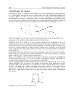
We begin with a study of simple angular velocity, where a body rotates about a fixed axis.
Specifically, let B be a rigid body rotating about an axis Z–Z fixed in both B and a reference
frame R as in Figure 4.4.1. Let n be a unit vector parallel to Z–Z as shown. Simple angular
velocity is then defined to be a vector parallel to n measuring the rotation rate of B in R.
To quantify this further, consider an end view of B and of axis Z–Z as in Figure 4.4.2.
Let X and Y be axes fixed in R and let L be a line fixed in B and parallel to the X–Y plane.
Let θ be an angle measuring the inclination of L relative to the X-axis as shown. Then, the
angular velocity ω (simple angular velocity) of B in R is defined to be:
(4.4.1)
where is sometimes called the angular speed of B in R.
FIGURE 4.3.8
Configuration graph defining the orientation
of B
in R (see Figure 4.3.7).
FIGURE 4.3.9
Configuration graph for a 1–3–1 rotation.
N
i
1
2
3

N
N
α
ˆ
i i
n
n
i i
ˆ
β
γ
N
i
1
2
3
N
N
ˆ
i i
n
n
i i
ˆ
θ
θ
θ
1
2 3
Nn n n

Nn n n
Nn n n
121232233
2 12 1 123 13 2 123 13 3
3 12 1 123 13 2 123 13 3
=+ −
=− + −
()
+− −
()
=− + +
()
+− +
()
cscss
cs ccc ss ccc sc
ss scc cs scs cc
nN N N
nN N N
nN N N
121122123
2 23 1 123 13 2 123 13 3
3 23 1 123 13 2 123 13 3
=+ −
=+−
()
++
()
=− + − −
()

+− +
()
ccsss
sc ccc ss scc cs
ss ccs sc scs cc
ωω
=
D
˙
θn
˙
θ
0593_C04*_fm Page 83 Monday, May 6, 2002 2:06 PM
84 Dynamics of Mechanical Systems
Observe that θ measures the rotation of B in R. It is also a measure of the orientation of
B in R. In this context, the angular velocity of B in R is a measure of the rate of change of
orientation of B in R.
The simple angular acceleration α of B in R is then defined as the time rate of change of
the angular velocity. That is,
(4.4.2)
If we express α and β in the forms:
(4.4.3)
then α, ω, and θ are related by the expressions:
(4.4.4)
By integrating we have the relations:
(4.4.5)
where θ
o
and ω
o

are values of θ and ω at some initial time t
o
.
From the chain rule for differentiation we have:
(4.4.6)
Then by integrating we obtain:
(4.4.7)
where, as before, ω
o
is an initial value of ω when θ is θ
o
. If α is constant, we have the
familiar relation:
(4.4.8)
FIGURE 4.4.1
A body B rotating in a reference frame R.
FIGURE 4.4.2
End view of body B.
B
Z
Z
n
R
Y
L
X
Z θ
B
n
ααωω==ddt

˙˙
θn
ααωω==αωnn and
ωθ αωθ===
˙

˙
˙˙
and
θωθ ωαω=+ =+
∫∫
dt dt
oo
and
αω ω ωθ θ ωωθ ω== =
()()
==
()
˙
d dt d d d dt d d d dt
2
2
ωαθω
22
2=+
∫
d
o
ωω αθ
22

2=+
o
0593_C04*_fm Page 84 Monday, May 6, 2002 2:06 PM
Kinematics of a Rigid Body 85
Example 4.4.1: Revolutions Turned Through During Braking
Suppose a rotor is rotating at an angular speed of 100 rpm. Suppose further that the rotor
is braked to rest with a constant angular deceleration of 5 rad/sec
2
. Find the number N
of revolutions turned through during braking.
Solution: From Eq. (4.4.8), when the rotor is braked to rest, its angular speed ω is zero.
The angle θ turned through during braking is, then,
Hence, the number of revolutions turned through is:
4.5 General Angular Velocity
Angular velocity may be defined intuitively as the time rate of change of orientation.
Generally, however, no single quantity defines the orientation for a rigid body. Hence,
unlike velocity, angular velocity cannot be considered as the derivative of a single quantity.
Nevertheless, it is possible to define the angular velocity in terms of derivatives of a set
of unit vectors fixed in the body. These unit vector derivatives thus provide a measure of
the rate of change of orientation of the body.
Specifically, let B be a body whose orientation is changing in a reference frame R, as
depicted in Figure 4.5.1. Let n
1
, n
2
, and n
3
be mutually perpendicular unit vectors as shown.
Then, the angular velocity of B in R, written as
R

ω
B
, is defined as:
(4.5.1)
The angular velocity vector has several properties that are useful in dynamical analyses.
Perhaps the most important is the property of producing derivatives by vector multipli-
cation: specifically, let c be any vector fixed in B. Then, the derivative of c in R is given
by the single expression:
(4.5.2)
FIGURE 4.5.1
A rigid body changing orientation in
a reference frame.
θωα π=− =−
()( )
[]
()
−
()
[]
==
o
2
2
2 2 100 60 2 5
10 966 628 3 radians degrees
N = 1 754.
RB
d
dt
d

dt
d
dt
ωω
=
⋅




+⋅




+⋅




D
n
nn
n
nn
n
nn
2
31
3

12
1
23
ddt
RB
cc=×ωω
B
R
n
n
n
3
2
1
0593_C04*_fm Page 85 Monday, May 6, 2002 2:06 PM
86 Dynamics of Mechanical Systems
To see this, let c be expressed in terms of the unit vectors n
1
, n
2
, and n
3
. That is, let
(4.5.3)
Because c is fixed in B, the scalar components c
i
(i = 1, 2, 3) are constants; hence, the
derivative of c in R is:
(4.5.4)
Next, consider the product

R
ω
B
× n
1
:
(4.5.5)
Recall that:
(4.5.6)
By differentiating these expressions we have:
(4.5.7)
Hence, Eq. (4.5.5) may be written as:
(4.5.8)
Because any vector V may be expressed as (V · n
1
)n
1
+ (V · n
2
)n
2
+ (V · n
3
)n
3
, we see that
the right side of Eq. (4.5.8) is an identity for dn
1
/dt. Thus, we have the result:
(4.5.9)

Similarly, we have the companion results:
(4.5.10)
Finally, by using these results in Eq. (4.5.4) we have:
(4.5.11)
cn n n=++ccc
11 22 33
d dt c d dt c dt c dtcnnn=++
1 1 22 33
RB
d
dt
d
dt
d
dt
d
dt
d
dt
ωω× = ⋅






+⋅







+⋅












×
=− ⋅






+⋅







n
n
nn
n
nn
n
nn n
n
nn
n
nn
1
2
31
3
12
1
23 1
3
13
1
22
nn nn
11 13
10⋅= ⋅= and
d
= 0 and
1
n

n
n
nn
n
11
31
3
dt
d
dt
d
dt
⋅⋅=−⋅
RB
d
dt
d
dt
d
dt
ωω× = ⋅






+⋅







+⋅






n
n
nn
n
nn
n
nn
1
1
11
1
22
1
33
RB
ddtωω× =nn
11
RB RB
ddt ddtωωωω×= ×=nn nn

22 33
and
ddtc c c
ccc
RB RB RB
RB
RB
cnnn
nnn
c
=×+×+×
=× + +
()
=×
112233
11 22 33
ωωωωωω
ωω
ωω


0593_C04*_fm Page 86 Monday, May 6, 2002 2:06 PM
Kinematics of a Rigid Body 87
Observe the pattern of the terms in Eq. (4.5.1). They all have the same form, and they
may be developed from one another by simply permuting the indices.
Example 4.5.1: Simple Angular Velocity
We may also observe that Eq. (4.5.1) is consistent with our earlier results on simple angular
velocity. To see this, let B rotate in R about an axis parallel to, say, n
1
, as shown in Figure

4.5.2. Let X–X be fixed in both B and R. Then, from Eq. (4.4.1), the angular velocity of B
in R is:
(4.5.12)
where, as before, θ measures the rotation angle. From Eq. (4.5.1), we see that
R
ω
B
may be
expressed as:
(4.5.13)
Because n
1
is fixed, parallel to axis X–X, its derivative is zero; hence, the third term in Eq.
(4.5.13) is zero. The first two terms may be evaluated using Eq. (3.5.7). Specifically,
(4.5.14)
By substituting into Eq. (4.5.13), we have:
(4.5.15)
which is identical to Eq. (4.5.11).
4.6 Differentiation in Different Reference Frames
Consider next the differentiation of a vector with respect to different reference frames.
Specifically, let V be the vector and let R and be two distinct reference frames. Let
i
be mutually perpendicular unit vectors fixed in , as represented in Figure 4.6.1. Let V
be expressed in terms of the
i
as:
(4.6.1)
FIGURE 4.5.2
Rotation of a body about a fixed
axis X–X

.
X
X
R
n
n
n
B
2
1
3
RB
ωω=
˙
θn
1
RB
d
dt
d
dt
d
dt
ωω= ⋅







+⋅






+⋅






n
nn
n
nn
n
nn
2
31
3
12
1
23
ddt ddtnnnn nnnn
2123 3132
=×= =×=−
˙˙

˙˙
θθ θ θ and
RB
ωω=
˙
θn
1
ˆ
R
ˆ
n
ˆ
R
ˆ
n
Vn n n=++
ˆ
ˆ
ˆ
ˆ
ˆ
ˆ
VVV
11 22 33
0593_C04*_fm Page 87 Monday, May 6, 2002 2:06 PM
88 Dynamics of Mechanical Systems
Because the
i
are fixed in , the derivative of V in is obtained by simply differen-

tiating the scalar components in Eq. (4.6.1). That is,
(4.6.2)
Next, relative to reference frame R, the derivative of V is:
(4.6.3)
where the second equality is determined from Eq. (4.6.2). Because the
i
are fixed in ,
the derivatives in R are:
(4.6.4)
Hence,
R
dV/dt becomes:
or
(4.6.5)
Because there were no restrictions on V, Eq. (4.6.5) may be written as:
(4.6.6)
where any vector quantity may be inserted in the parentheses.
FIGURE 4.6.1
Vector V and reference frames R
and
ˆ
R.
R
R
V
n
n
n
ˆ
ˆ

ˆ
ˆ
3
2
1
ˆ
n
ˆ
R
ˆ
R
ˆ
ˆ
ˆ
ˆ
ˆ
ˆ
ˆ
R
ddt dVdt dVdt dVdtVnnn=
()
+
()
+
()
11 22 33
RR
RR
RR R R
ddt dVdt Vd dtdVdt

V d dt dV dt V d dt
d dtVd dtVd dtVd dt
Vnn n
nnn
Vn n n
=
()
++
()
++
()
+
=+ + +
ˆ
ˆ
ˆ
ˆ
ˆ
ˆ
ˆ
ˆ
ˆ
ˆ
ˆ
ˆ
ˆ
ˆ
ˆˆ
ˆ
ˆ

1111 22
23 3 333
11 22 33
ˆ
n
ˆ
R
RRR
i
ddt i
ˆˆ
,,
ˆ
nn
1
123=× =
()
ωω
R R RR RR
RR
RRR
ddt ddtV V
V
ddt V V V
VV n n
n
Vnnn
=+×+×
+×
=+×++

()
ˆˆˆ
ˆ
ˆˆ
ˆˆ
ˆ
ˆ
ˆ
ˆ
ˆ
ˆ
ˆ
1122
33
11 22 33
ωωωω
ωω
ωω
RRRR
ddt ddtVV V=+×
ˆˆ
ωω
RRRR
ddtddt
()
=
()
+×
()
ˆˆ

ωω
0593_C04*_fm Page 88 Monday, May 6, 2002 2:06 PM
Kinematics of a Rigid Body 89
Example 4.6.1: Effect of Earth Rotation
Equation (4.6.6) is useful for developing expressions for velocity and acceleration of
particles moving relative to rotating bodies. To illustrate this, consider the case of a rocket
R launched vertically from the Earth’s surface. Let the vertical speed of R relative to the
Earth (designated as E) be V
0
. Suppose we want to determine the velocity of R in an
astronomical reference frame A in which E rotates for the cases when R is launched from
(a) the North Pole, and (b) the equator.
Solution: Consider a representation of R, E, and A as in Figure 4.6.2a and b, where i,
j, and k are mutually perpendicular unit vectors fixed in E, with k being along the
north/south axis, the axis of rotation of E. In both cases the velocity of R in A may be
expressed as:
(4.6.7)
where O is the center of the Earth which is also fixed in A.
a. For launch at the North Pole, the position vector OR is simply (r + h)k, where
r is the radius of E (approximately 3960 miles) and h is the height of R above
the surface of E. Thus, from Eq. (4.6.6),
A
V
R
is:
(4.6.8)
Observe that angular velocity of E in A is along k with a speed of one revolution
per day. That is,
(4.6.9)
Hence, by substituting into Eq. (4.6.8), we have:

(4.6.10)
FIGURE 4.6.2
Vertical launch of a rocket from the surface of the Earth. (a) Launch at the North Pole; (b) launch at the Equator.
O
N
S
k
j
i
A
R
V
0
(a)
O
N
S
k
j
i
A
R
V
0
(b)
AR A
ddtVOR=
AR E AE
dr h dt r hVk k=+
()

[]
+×+
()
ωω
AE
ωω= =
()( )
=×
−
ω
π
kkk
2
24 3600
727 10
5
. rad sec
AR
o
hVV==
˙
kk
0593_C04*_fm Page 89 Monday, May 6, 2002 2:06 PM
90 Dynamics of Mechanical Systems
b. For the launch at the Equator, the position vector OR is (r + h)i. In this case, Eq.
(4.6.7) becomes:
or
(4.6.11)
Observe that h is small (at least, initially) compared with r. Thus, a reasonable
approximation to

A
V
R
is:
(4.6.12)
Observe also the differences in the results of Eqs. (4.6.10) and (4.6.11).
4.7 Addition Theorem for Angular Velocity
Equation (4.6.6) is useful for establishing the addition theorem for angular velocity — one
of the most important equations of rigid body kinematics. Consider a body B moving in
a reference frame , which in turn is moving in a reference frame R as depicted in Figure
4.7.1. Let V be an arbitrary vector fixed in B. Using Eq. (4.6.6), the derivative of V in R is:
(4.7.1)
Because V is fixed in B its derivatives in R and may be expressed in the forms (see
Eq. (4.5.2)):
(4.7.2)
FIGURE 4.7.1
Body B moving in reference frame
R and
ˆ
R.
AR E AE
o
dr h dt r h
hrh
Vh
Vi i
ij
ij
=+
()

+×+
()
=++
()
=+
()()
+
[]
×
()
−
ω
ω
˙
.3960 5280 7 27 10
5
AR
o
VhVi j=+ +
()
1520 ω ft sec
AR
O
VVi j=+1520 ft sec
ˆ
R
RRRR
ddt ddtVV V=+×
ˆˆ
ωω

ˆ
R
RRR RRB
ddt ddtVVVV=× =×ωωωω
ˆˆ
and
B
R
R
ˆ
V
0593_C04*_fm Page 90 Monday, May 6, 2002 2:06 PM
Kinematics of a Rigid Body 91
Hence, by substituting into Eq. (4.7.1) we have:
or
(4.7.3)
Because V is arbitrary, we thus have:
or
(4.7.4)
Equation (4.7.4) is an expression of the addition theorem for angular velocity. Because
body B may itself be considered as a reference frame, Eq. (4.7.4) may be rewritten in the
form:
(4.7.5)
Equation (4.7.5) may be generalized to include reference frames. That is, suppose a
reference frame R
n
is moving in a reference frame R
0
and suppose that there are (n –1)
intermediate reference frames, as depicted in Figure 4.7.2. Then, by repeated use of

Eq. (4.7.5), we have:
(4.7.6)
The addition theorem together with the configuration graphs of Section 4.3 are useful
for obtaining more insight into the nature of angular velocity. Consider again a body B
moving in a reference frame R as in Figure 4.7.3. Let the orientation of B in R be described
by dextral orientation angles α, β, and γ. Let n
i
and N
i
(i = 1, 2, 3) be unit vector sets fixed
in B and R, respectively. Then, from Figure 4.3.8, the configuration graph relating n
i
and
FIGURE 4.7.2
A set of n + 1 reference frames.
FIGURE 4.7.3
A body B moving in a reference frame R.
RB RB RR
ωωωωωω×= ×+ ×VVV
ˆˆ
RBRBRR
ωωωωωω−−
()
×=
ˆˆ
V 0
RBRBRR
ωωωωωω−− =
ˆˆ
0

RB RBRR
ωωωωωω=+
ˆˆ
RR RRRR
02 0112
ωωωωωω=+
RR RRRR R R
nnn00112 1
ωωωωωωωω=+++
−



R
R
R
R
R
n-1
n
2
1
0
R
N
N
N
B
n
n

n
3
2
1
3
2
1
0593_C04*_fm Page 91 Monday, May 6, 2002 2:06 PM
92 Dynamics of Mechanical Systems
N
i
is as reproduced in Figure 4.7.4. Recall that the unit vector sets
i
and
i
are fixed
in intermediate reference frames R
1
and R
2
used in the development of the configuration
graph. The horizontal lines in the graph signify axes of simple angular velocity (see Section
4.4) of adjoining reference frames. The respective rotation angles are written at the base
of the graph. Therefore, from Eq. (4.7.6) we have:
(4.7.7)
From the configuration graph of Figure 4.7.4 we have (see Eq. (4.4.1)):
(4.7.8)
Hence,
R
ω

B
is:
(4.7.9)
Finally, using the analysis associated with the configuration graph (see Eqs. (4.3.6) and
(4.3.7)), we can express
R
ω
B
as:
(4.7.10)
or alternatively as:
(4.7.11)
Example 4.7.1: A Simple Gyro
(See Reference 4.1.) A circular disk (or gyro), D, is mounted in a yoke (or gimbal), Y, as
shown in Figure 4.7.5. Y is mounted on a shaft S and is free to rotate about an axis that
is perpendicular to S. S in turn can rotate about its own axis in bearings fixed in a reference
frame R. Let D have an angular speed Ω relative to Y; let the rotation of Y in S be measured
by the angle φ; and let the rotation of S in R be measured by the angle ψ. Let N
Yi
and N
Ri
be configured so that when Y is vertical and when the plane of D is parallel to S, the unit
vector sets are mutually aligned. Also in this configuration, let the orientation angles φ
and ψ be zero. Determine the angular velocity of D in R by constructing a configuration
graph as in Figure 4.7.4 and by using the addition theorem of Eq. (4.7.6).
FIGURE 4.7.4
Configuration graph relating n
i
and N
i

.
N
i
1
2
3
N
N
α
ˆ
i i
n
n
i i
ˆ
β
γ
R R R B
1 2
ˆ
N
ˆ
n
RB RR R R R B
ωωωωωωωω=++
11 22
RR R R RB
ωωωωωω
112
11 22 33

== == ==
˙˙
ˆ
,
˙
ˆ
˙
ˆ
,
˙
ˆ
˙
αα ββ γγNN Nn nn
RB
ωω= + + = + +
˙
˙
ˆ
˙
ˆ
˙
ˆ
˙
ˆ
˙
αβγαβγNNn Nnn
123 123
RB
sccs sccωω= +
()

+−
()
+−
()
˙
˙
˙
˙
˙
˙
αγ β γ β γ
β
α
β
αα
β
α
NNN
123
RB
cc s c cs sωω= +
()
+−
()
++
()
˙
˙˙
˙˙
˙

αβ βα αγ
β
γγ γ
β
γ
β
nnn
123
0593_C04*_fm Page 92 Monday, May 6, 2002 2:06 PM
Kinematics of a Rigid Body 93
Solution: Let Ω be the derivative of a rotation angle θ of D in Y; let N
Di
(i = 1, 2, 3) be
mutually perpendicular unit vectors fixed in D; and let the N
Di
be mutually aligned with
the N
Yi
when θ is zero. Similarly, let N
Si
(i = 1, 2, 3) be mutually perpendicular unit vectors
fixed in S which are aligned with the N
Ri
when ψ is zero. Then, a configuration graph
representing the various unit vector sets and the orientation angles can be constructed, as
shown in Figure 4.7.6. From this graph and from Eq. (4.7.6), the angular velocity of D in
R may be expressed as:
(4.7.12)
The configuration graph is useful for expressing
R

ω
D
solely in terms of one of the unit
vector sets. For example, in terms of the yoke unit vectors N
Yi
,
R
ω
D
is:
(4.7.13)
where Ω is (see also Problem P4.7.1).
4.8 Angular Acceleration
The angular acceleration of a body B in a reference frame R is defined as the derivative
in R of the angular velocity of B in R. Specifically,
(4.8.1)
Unfortunately, there is not an addition theorem for angular acceleration analogous to that
for angular velocity. That is, in general,
(4.8.2)
FIGURE 4.7.5
A spinning disk D and a supporting yoke Y and shaft S.
FIGURE 4.7.6
Configuration graph for the system of Figure 4.7.5.
i
1
2
3
N N N
N
Ri

Si
Yi
Di
ψ
φ
θ
RD
RSY
ωω= + +
˙
˙
˙
ψφθNNN
231
RD
YYY
scωω= +
()
++Ω
˙˙
˙
ψψφ
φφ
NNN
123
˙
θ
RB RRB
ddt ddtααωωααωω= or =
R

R
R
RRR
RR
nnn
00
112
1
αααααααα≠+++
−
K
0593_C04*_fm Page 93 Monday, May 6, 2002 2:06 PM
94 Dynamics of Mechanical Systems
To see this, consider three reference frames R
0
, R
1
, and R
2
as in Eq. (4.7.5):
(4.8.3)
By differentiating in R
0
we obtain:
or
(4.8.4)
Consider the last term: From Eq. (4.6.6) we have:
(4.8.5)
Then, by substituting into Eq. (4.8.4) we have:
(4.8.6)

Hence, unless is zero, the addition theorem for angular acceleration does not
hold as it does for angular velocity. However, if is zero (for example, if
are parallel), then the addition theorem for angular acceleration holds as
well. This occurs if all rotations of the reference frames are parallel, or, equivalently, if all
the bodies (treated as reference frames) move parallel to the same plane.
In some occasions the angular acceleration of a body B in a reference frame R (
R
α
B
) may
be computed by simply differentiating the scalar components of the angular velocity of
B in R (
R
ω
B
). This occurs if
R
ω
B
is expressed either in terms of unit vectors fixed in R or in
terms of unit vectors fixed in B. To see this, consider first the case where the limit vectors
of
R
ω
B
are fixed in R. That is, let N
i
(i = 1, 2, 3) be mutually perpendicular unit vectors
fixed in R and let
R

ω
B
be expressed as:
(4.8.7)
Then, because the N
i
are fixed in R, their derivatives in R are zero. Hence, in this case,
R
α
B
becomes:
(4.8.8)
Next, consider the case where the unit vectors of
R
ω
B
are fixed in B. That is, let n
i
(i =
1, 2, 3) be mutually perpendicular unit vectors fixed in B and let
R
ω
B
be expressed as:
(4.8.9)
R
R
R
RRR
0

2
0
11 2
ωωωωωω=+
RR
R
RR
R
R
RR
d dt d dt d dt
00
2
00
1
0
12
ωωωωωω=+
R
R
R
R
R
RR
ddt
0
2
0
1
0

12
ααααωω=+
R
RR RRR
R
RR R
RR
R
RR R
ddtddt
0
12 112
0
11 2
12
0
11 2
ωωωωωωωω
ααωωωω
=+×
=+×
R
R
R
RRR
R
RR R
0
2
0

11 2
0
11 2
ααααααωωωω=++×
R
RR R
0
11 2
ωωωω×
R
RR R
0
11 2
ωωωω×
R
RRR
0
112
ωωωωand
RB
ωω= + +ΩΩΩ
11 22 33
NNN
RB
αα= + +
˙˙˙
ΩΩΩ
11 22 33
NNN
RB

ωω= + +ωωω
11 22 33
nnn
0593_C04*_fm Page 94 Monday, May 6, 2002 2:06 PM
Kinematics of a Rigid Body 95
Then
R
α
B
is:
(4.8.10)
Observe that the last three terms each involve derivatives of unit vectors fixed in B. From
Eq. (4.5.2) these derivatives may be expressed as:
(4.8.11)
Hence, the last three terms of Eq. (4.8.10) may be expressed as:
(4.8.12)
Therefore,
R
αα
αα
B
becomes:
(4.8.13)
Example 4.8.1: A Simple Gyro
See Example 4.7.1. Consider again the simple gyro of Figure 4.7.5 and as shown in Figure
4.8.1. Recall from Eq. (4.7.13) that the angular velocity of the gyro D in the fixed frame R
may be expressed as:
(4.8.14)
where as before Ω (the gyro spin) is ; φ and ψ are orientation angles as shown in Figure
4.8.1; and N

Y1
, N
Y2
, and N
Y3
are unit vectors fixed in the yoke Y. Determine the angular
acceleration of D in R.
Solution: By differentiating in Eq. (4.4.14) we obtain:
(4.8.15)
RB RRB R
RR
RRR
ddt wddt
ddt ddt
d dt d dt d dt
ααωω==+ +
+++
=++
++ +
˙˙
˙
˙˙˙
ωω
ωωω
ωωω
ωωω
11 1 1 22
22 3333
11 22 33
11 22 33

nn n
nnn
nnn
nnn
R
i
RB
i
ddt inn=× =
()
ωω ,,123
ωωω
ωωω
ωωω
ωωω
11 22 33
112233
11 22 33
11 22 33
0
RRR
RB RB RB
RB RB RB
RB
RBRB
d dt d dt d dtnnn
nnn
nnn
nnn
++

=×+×+×
=× +× +×
=× + +
()
=× =




ωωωωωω
ωωωωωω
ωω
ωωωω
RB
αα= + +
˙˙˙
ωωω
11 22 33
nnn
RD
YYY
scωω= +
()
++Ω
˙˙
˙
ψψφ
φφ
NNN
123

˙
θ
RD
Y
R
Y
Y
R
Y
Y
R
Y
sc sddt
cs cddt
ddt
αα= + +
()
++
()
+−
()
+
++
˙
˙˙ ˙
˙
˙
˙˙
˙
˙

˙˙
ΩΩψψφ ψ
ψψφ ψ
φφ
φφ φ
φφ φ
NN
NN
NN
11
22
33
0593_C04*_fm Page 95 Monday, May 6, 2002 2:06 PM
96 Dynamics of Mechanical Systems
Because the N
Yi
(i = 1, 2, 3) are fixed in the yoke Y, their derivatives may be evaluated
from the expression:
(4.8.16)
where from Eqs. (4.7.12) and (4.7.13)
R
ωω
ωω
Y
is:
(4.8 17)
Hence, the
R
dN
Yi

/dt are:
(4.18)
and, by substitution into Eq. (4.8.15),
R
α
D
becomes:
(4.19)
Comment: Observe that by comparing Eqs. (4.8.14) and (4.8.19) we see that
R
αα
αα
D
is
considerably longer and more detailed than
R
ωω
ωω
D
. This raises the question as to whether a
different unit vector set might produce a simpler expression for
R
αα
αα
D
. Unfortunately, this
is not the case, as seen in Problem P4.8.2. It happens that the N
Yi
are the preferred unit
vectors for simplicity.

FIGURE 4.8.1
The gyro of Figure 4.7.5.
R
Yi
RY
Yi
ddt iNN=× =
()
ωω , ,123
RY
RS Y YY
scωω= + = + +
˙
˙
˙˙
˙
ψφψ ψ φ
φφ
NN N NN
23 1 2 3
R
YYY
R
YYY
R
YYY
ddt c
ddt s
ddtc s
NNN

NNN
NNN
123
213
312
=−
=− +
=−
˙
˙
˙
˙
˙˙
φψ
φψ
ψψ
φ
φ
φφ
RD
YY
Y
sc c s
c
αα= + +
()
++−
()
+−
()

˙
˙˙
˙
˙˙˙
˙
˙
˙
˙˙
˙
ΩΩ
Ω
ψφψ ψ φψφ
φψ
φφ φ φ
φ
NN
N
12
3
0593_C04*_fm Page 96 Monday, May 6, 2002 2:06 PM
Kinematics of a Rigid Body 97
4.9 Relative Velocity and Relative Acceleration of Two Points
on a Rigid Body
Consider a body B moving in a reference frame R as in Figure 4.9.1. Let P and Q be points
fixed in B. Consider the velocity and acceleration of P and Q and their relative velocity
and acceleration in reference frame R. Let O be a fixed point (the origin) of R. Let vectors
p and q locate P and Q relative to O and let vector r locate P relative to Q. Then, from
Figure 4.9.1, these vectors are related by the expression:
(4.9.1)
By differentiating we have:

(4.9.2)
Because P and Q are fixed in B, r is fixed in B. Hence, from Eq. (4.5.2), we have:
(4.9.3)
Then, by substituting into Eq. (4.9.2), we have:
(4.9.4)
By differentiating in Eq. (4.9.4), we obtain the following relations for accelerations:
(4.9.5)
and
(4.9.6)
FIGURE 4.9.1
A body B moving in a reference
frame R with points P and Q fixed
in B.
pqr=+
RPRQ R RPRQ R RPQ
ddt ddtVV r VV r V=+ −= = or
RRB
ddtrr=×ωω
RPQRB RPRQRQ
VrVVr=× =+×ωωωω or
RPQRB R B R B
ar r=×+× ×
()
ααωωωω
RP RQ R B R B R B
aa r r=+ ×+ × ×
()
ααωωωω
Q
P

R
O
q
p
r
B
0593_C04*_fm Page 97 Monday, May 6, 2002 2:06 PM
98 Dynamics of Mechanical Systems
Equations (4.9.4) and (4.9.6) are sometimes used to provide an interpretation of rigid
body motion as being a superposition of translation and rotation. Specifically, at any
instant, from Eq. (4.9.4) we may envision a body as translating with a velocity V
Q
and
rotating about Q with an angular velocity
R
ωω
ωω
B
.
Example 4.9.1: Relative Movement of a Sports Car Operator’s Hands During
a Simple Turn
To illustrate the application of Eqs. (4.9.4) and (4.9.5), suppose a sports car operator
traveling at a constant speed of 15 miles per hour, with hands on the steering wheel at 10
o’clock and 2 o’clock, is making a turn to the right with a turning radius of 25 feet. Suppose
the steering wheel has a diameter of 12 inches and is in the vertical plane. Suppose further
that the operator is turning the steering wheel at one revolution per second. Find the
velocity and acceleration of the motorist’s left hand relative to the right hand.
Solution: Let the movement of the car be represented as in Figure 4.9.2, and let the
steering wheel be represented as in Figure 4.9.3, where n
x

, n
y
, and n
z
are mutually per-
pendicular unit vectors fixed in the car. Let n
x
be forward; n
z
be vertical, directed up; and
n
y
be to the left. Let W represent the steering wheel, C represent the car, and S the road
surface (fixed frame). Let O represent the center of W, and let L and R represent the
motorist’s left and right hands. The desired relative velocity and acceleration (
S
V
L/R
and
s
a
L/R
) may be obtained directly from Eqs. (4.9.4) and (4.9.5) once the angular velocity and
the angular acceleration of W are known. From the addition theorem for angular velocity
(Eq. (4.7.6)), the angular velocity of the steering wheel W in S is:
(4.9.7)
From the data presented, the angular velocity of the car C in S is:
(4.9.8)
where V is the speed of C (15 mph or 22 ft/sec) and ρ is the turn radius. Similarly, the
angular velocity of the steering wheel W in C is:

(4.9.9)
Hence,
S
ωω
ωω
W
is:
(4.9.10)
FIGURE 4.9.2
Sports car C entering a turn to the
right.
SWCWSC
ωωωωωω=+
SC
zz
Vωω=−
()
=−
()
ρ nn22 25 rad sec
CW
x
ωω=2πn rad sec
SW
xz
ωω= −
()
22225πnnrad sec
25 ft
25 ft

C 15 mph
n
n
n
x
y
z
0593_C04*_fm Page 98 Monday, May 6, 2002 2:06 PM
Kinematics of a Rigid Body 99
By differentiating in Eq. (4.9.10), the angular acceleration of W in S is:
(4.9.11)
Finally, from Eqs. (4.9.4) and (4.9.5), the desired relative velocity and acceleration expres-
sions are:
(4.9.12)
and
(4.9.13)
Example 4.9.2: Absolute Movement of Sports Car Operator’s Hands
To further illustrate the application of Eqs. (4.9.4) to (4.9.6), suppose we are interested in
determining the velocity and acceleration of the sports car operator’s left hand in the
previous example. Specifically, find the velocity and acceleration of L in S.
Solution: Observe that the steering wheel hub O is fixed in both the steering wheel W
and the car C. Observe further that O moves on the 25-ft-radius curve (or circle) at 15
mph (or 22 ft/sec). Therefore, the velocity and acceleration of O are:
(4.9.14)
By knowing
S
V
O
and
S

a
O
, we can use Eqs. (4.9.4) and (4.9.6) to determine
S
V
L
and
S
a
L
. That is,
and
(4.9.15)
where from Figure 4.9.3 the position vector OL is:
(4.9.16)
Hence, from Eqs. (4.9.10), (4.9.11), and (4.9.14),
S
V
L
and
S
a
L
are seen to be:
SW S
x
SC
xy
ddtααωω=+=×=−
()

()
2 0 2 2 22 25πππnnn
SLRSW
xz y
xz
VRLnnn
nn
=×= −
()
[]
×
()
=+
ωω 22225 32
0 762 5 44
π
. . ft sec
SLR SW S W S W
yyx zxz
y
aRL RL
ft sec
2
=×+× ×
()
=−
()
×
()
+−

()
[]
×+
()
=−
ααωωωω
2 22 25 3 2 2 22 25 0 762 5 44
33 5
ππnnn nnn
n

.
SO
x
SO
yy
Vn a n n==−
()
=−22 22 25 19 36
2
ft sec and .
SLSOSW
OLVV=+ ×ωω
SLSO SW S W S W
a a OL OL=+ ×+ × ×
()
ααωωωω
OL n n n n=
()
+

()
=+05 0866 05 0433 025 . . .
yz y z
SL
xx z y z
Vn n n n n=+ −
()
×+
()
22 2 22 25 0 433 0 25π
0593_C04*_fm Page 99 Monday, May 6, 2002 2:06 PM
100 Dynamics of Mechanical Systems
or
(4.9.17)
and
(4.9.18)
Example 4.9.3: A Rod with Constrained End Movements
As a third example illustrating the use of Eqs. (4.9.4) and (4.9.6) consider a rod whose
ends A and B are restricted to movement on horizontal and vertical lines as in Figure 4.9.4.
Let the rod have length 13 m. Let the velocity and acceleration of end A be:
(4.9.19)
where n
x
, n
y
, and n
z
are unit vectors parallel to the coordinate axes as shown. Let the
angular velocity and angular acceleration of the rod along the rod itself be zero. That is,
(4.9.20)

where n is a unit vector along the rod. Find the velocity and acceleration of end B for the
rod position shown in Figure 4.9.4.
FIGURE 4.9.3
Sports car steering wheel W and
left and right hands L and R.
FIGURE 4.9.4
A rod AB with constrained motion
of its ends.
1 rev/sec
R
W
O
6 in
L
n
n
n
z
x
y
30°
30°
SL
xyz
Vnnn=−+22 381 1 571 2 721. . . ft sec
SL
yyyz
xz xz yz
xyz
an nnn

nn nn nn
nnn
=− + −
()
×+
()
+−
()
×−
()
×+
()
[]
=− − −
19 36 5 529 0 433 0 25
6 283 0 88 6 283 0 88 0 433 0 25
2 765 36 79 9 87


. . . ft sec
2
Vn a n
A
x
A
x
==−63
2
m s and m s
ωωαα

AB AB
⋅= ⋅=nn00 and
O
X
Y
Z
B
n
n
n
A
3 m
4 m
12 m
z
y
x
0593_C04*_fm Page 100 Monday, May 6, 2002 2:06 PM
Kinematics of a Rigid Body 101
Solution: From Eq. (4.9.4), the velocity of end B may be expressed as:
(4.9.21)
For the rod position of Figure 4.9.4, AB is:
(4.9.22)
Let ωω
ωω
AB
be expressed in the form:
(4.9.23)
Let V
B

be expressed as:
(4.9.24)
Then, by substituting from Eqs. (4.9.19), (4.9.22), (4.9.23), and (4.9.24) we have:
(4.9.25)
Also, from Eq. (4.9.20) we have:
(4.9.26)
Equations (4.9.25) and (4.9.26) are equivalent to the following four scalar equations for ω
x
,
ω
y
, ω
z
, and v
B
:
(4.9.27)
Solving for ω
x
, ω
y
, ω
z
, and v
B
, we obtain:
(4.9.28)
and
(4.9.29)
VV AB

BAAB
=+ ×ωω
AB n n n=− + +4123
xyz
m
ωω
AB
xx yy zz
=++ωωωnnn
Vn
BB
z
v=
v
B
zx y zx xzy
xyz
nn n n
n
=+ −
()
+− −
()
++
()
6312 34
12 4
ωω ωω
ωω
−+ + =41230ωωω

xyz
03120 6
30400
12 4 0 0
412300
ωω ω
ωωω
ωωω
ωωω
xy z
B
xyz
B
xyz
B
xyz
B
v
v
v
v
+− +=−
−+ −+=
++−=
−+ + +=
ωωω
xy
=− =− =−0 568 0 296 0 426
3
., ., .rad sec rad sec rad sec

v
B
=−8m s
0593_C04*_fm Page 101 Monday, May 6, 2002 2:06 PM
102 Dynamics of Mechanical Systems
Similarly, from Eq. (4.9.6), the acceleration of end A may be expressed as:
(4.9.30)
Let α
AB
be expressed in the form:
(4.9.31)
Let a
B
be expressed as:
(4.9.32)
Then, by substituting from Eqs. (4.9.19), (4.9.22), (4.9.23), (4.9.31), and (4.9.32) into (4.9.30),
we have:
(4.9.33)
Also, from Eq. (4.9.20) we have:
(4.9.34)
Using Eq. (4.9.29) for values of ω
x
, ω
y
, and ω
z
, Eqs. (4.9.33) and (4.9.34) are equivalent to
the following four scalar equations for α
x
, α

y
, α
z
, and a
B
:
(4.9.35)
Solving for α
x
, α
y
, α
z
, and a
B
, we obtain:
(4.9.36)
and
(4.9.37)
a a AB AB
A B AB AB AB
=+ × + × ×
()
ααωωωω
αα
AB
xx yy zz
=++αααnnn
an
BB

z
a=
a
B
zxyzx xzy
xyzyx xzyyz
nn n n
nn nn
=− + −
()
+− −
()
++
()
−+−
()
+
3312 34
12 4 8 8 6 6
αα αα
αα ω ωω ω
−+ + =41230ααα
xyz
0 3 12 0 0 632
304071
12 4 0 1 776
412300
αα α
ααα
ααα

ααα
xy z
B
xyz
B
xyz
B
xyz
B
a
a
a
a
+− +=
−+ −+=
++−=
−+ + +=
.
.
.
ααα
xyz
=− =− =−2 083 0 641 0 213., ., .rad sec rad sec rad sec
222
a
B
=−29 33.ms
0593_C04*_fm Page 102 Monday, May 6, 2002 2:06 PM
Kinematics of a Rigid Body 103
4.10 Points Moving on a Rigid Body

Consider next a point P moving on a body B which in turn is moving in a reference frame
R as depicted in Figure 4.10.1. Let Q be a point fixed in B. Let p and q be position vectors
locating P and Q relative to a fixed point O in R. Let vector r locate P relative to Q. Then,
from Figure 4.10.1, we have:
(4.10.1)
By differentiating, we obtain:
(4.10.2)
where, as before,
R
V
P
and
R
V
Q
represent the velocities of P and Q in R. From Eq. (4.6.6),
R
dr/dt is:
(4.10.3)
Because Q is fixed in B, and because r locates P relative to Q,
R
dr/dt is the velocity of P
in B. Hence,
R
V
P
becomes:
(4.10.4)
Suppose that an instant of interest P happens to coincide with Q. Then, at that instant,
r is zero and

R
V
P
is:
(4.10.5)
Observe that at any instant there always exists a point P
*
, fixed in B, which coincides
with P. Therefore, Eq. (4.10.5) may be rewritten as:
(4.10.6)
FIGURE 4.10.1
A point P moving on a body B,
moving in reference frame R.
pqr=+
RPRQ
R
ddtVV r=+
RB
RR
ddt ddtrr r=+×ωω
RPRQBPRB
VVV r=++×ωω
RPBPRQ
VVV=+
RPBPRP
VVV=+
*
Q
P
R

O
q
p
r
B
0593_C04*_fm Page 103 Monday, May 6, 2002 2:06 PM
104 Dynamics of Mechanical Systems
By differentiating in Eq. (4.10.4), we can obtain a relation determining the acceleration
of P. That is,
(4.10.7)
where, as before,
R
a
P
and
R
a
Q
are the acceleration of P and Q in R, and
R
α
B
is the acceleration
of B in R. By using Eq. (4.6.6), we can express
R
d
B
V
P
/dt as:

(4.10.8)
Then, by using Eq. (4.10.3),
R
a
P
may be written as:
or
(4.10.9)
Suppose again that at an instant of interest P happens to coincide with Q. Then, r is
zero and
R
a
P
is:
(4.10.10)
Hence, in general, if P
*
is the point of B coinciding with P we have:
(4.10.11)
The term 2
R
ωω
ωω
B
×
B
V
P
is called the Coriolis acceleration, after the French mechanician de
Coriolis (1792–1843) who is credited with being the first to discover it. We have already

seen this term in our analysis of the movement of a point in a plane in Chapter 3 (see Eq.
(3.8.7)). This term is not generally intuitive, and it often gives rise to surprising and
unexpected effects.
Example 4.10.1: Movement of Sports Car Operator’s Hands
Equations (4.10.6) and (4.10.11) may also be used to determine the velocity and acceleration
of the sports car operator’s left hand of Example 4.9.2. Recall that the sports car is making
a turn to the right at 15 mph with a turn radius of 25 feet, and that the operator’s left
hand is at 10 o’clock on a 12-in diameter vertical steering wheel, as in Figures 4.10.2 and
4.10.3. Recall further that the operator is turning the wheel clockwise at one revolution
per second, as in Figure 4.10.3.
Solution: From Eq. (4.10.6), the velocity of the left hand L may be expressed as:
(4.10.12)
RP RQ RB P R B R B R
ddt ddtaa V r r=+ +×+×ααωω
RBP BB P RBB PBPRBB P
ddtddtVV VaV=+×=+×ωωωω
RPRQBPRBBPRB RB B P RB
aaa V r V r=++++ ×+ × × ×
()
[]
ωωααωωωω
RPBPRQ RBBPRB RB RB
aaa V r r=+ + × + ×+ × ×
()
2 ωωααωωωω
RPBP RQ R BB P
aaa V=+ + ×2 ωω
RPBP RP R BB P
aaa V=+ + ×
*

2 ωω
SLCLSL
VVV=+
*
0593_C04*_fm Page 104 Monday, May 6, 2002 2:06 PM
Kinematics of a Rigid Body 105
where L
*
is that point of the car C where L is located at the instant of interest and where,
as before, S is the fixed road surface. From Figure 4.10.3,
C
V
L
is:
(4.10.13)
From Figure 4.10.2,
S
V
L*
is:
(4.10.14)
Therefore, by substituting into Eq. (4.10.12), the velocity of L is:
(4.10.15)
In like manner, from Eq. (4.10.11), the acceleration of L is:
(4.10.16)
From Figure 4.10.3,
C
a
L
is:

(4.10.17)
FIGURE 4.10.2
Sports car C entering a turn to the right.
FIGURE 4.10.3
Sports car steering wheel W and left hand L.
25 ft
25 ft
C 15 mph
n
n
n
x
y
z
1 rev/sec
W
O
6 in
L
n
n
z
x
y
n
CLCW
xyz
yz
VOLnnn
nn

=×= × +
()
=− +
ωω 2 0 433 0 25
1 571 2 71
π
. . ft sec
SLSOSC
xz yz
x
VV OL
nn nn
n
*
.
.
=+×
=+ × +
()
=
ωω
22 0 88 0 433 0 25
22 381 ft sec
SL
xyz
Vnnn=−+22 381 1 571 2 71. . . ft sec
SLCLSL S CC L
aaa V=+ + ×
*
2 ωω

CLCW C W
xxyz
yz
aOLnnnn
nn
=× ×
()
=× × +
()
[]
=− −
ωωωω 6 238 6 283 0 433 0 25
17 095 9 87

. . ft sec
2
0593_C04*_fm Page 105 Monday, May 6, 2002 2:06 PM
106 Dynamics of Mechanical Systems
From Figure 4.10.2,
S
a
L*
is:
(4.10.18)
Finally, from both figures 2
S
ω
C
×
C

V
L
is:
(4.10.19)
Therefore, by substituting into Eq. (4.10.16), the acceleration of L is:
(4.10.20)
4.11 Rolling Bodies
Rolling motion is an important special case in the kinematics of rigid bodies. It is partic-
ularly important in machine kinematics. Rolling can occur between two bodies or between
a body and a surface. Rolling between two bodies occurs when the bodies are moving
relative to each other but still are in contact with each other, with the contacting points
having zero relative velocity. Similarly, a body rolls on a surface when it is moving relative
to the surface but is still in contact with the surface with the contacting point (or points)
having zero velocity relative to the surface.
Rolling may be defined analytically as follows: Let S be a surface and let B be a body
that rolls on S as depicted in Figure 4.11.1. (S could be a portion of a body upon which B
rolls.) Let B and S be counterformal so that they are in contact at a single point. Let C be
the point of B that is in contact with S. Rolling then occurs when:
(4.11.1)
FIGURE 4.11.1
A body B rolling on a surface S.
SL SOS C S C
yz z yz
y
aa OL
nn n nn
n
*

.

=+ × ×
()
=− + −
()
×−
()
×+
()
[]
=−
ωωωω
19 36 0 88 0 88 0 433 0 25
19 7 ft sec
2
2 2 088 1571 271
2 765
SCC L
zyz
x
ωω× = −
()
×− +
()
=−
Vnnn
n

. ft sec
2
SL

xyz
annn=− − −2 765 36 79 9 87. . . ft sec
2
SC
V = 0
B
P
p
C
0593_C04*_fm Page 106 Monday, May 6, 2002 2:06 PM