Advances in Robot Navigation Part 2 docx
Bạn đang xem bản rút gọn của tài liệu. Xem và tải ngay bản đầy đủ của tài liệu tại đây (2.11 MB, 20 trang )
Conceptual Bases of Robot Navigation Modeling, Control and Applications
9
For mobile robots, the architectures are defined by the control system operating principle.
They are constrained at one end by fully reactive systems (Kaelbling, 1986) and, in the other
end, by fully deliberative systems (Fikes & Nilsson, 1971). Within the fully reactive and
deliberative systems, lies the hybrid systems, which combines both architectures, with
greater or lesser portion of one or another, in order to generate an architecture that can
perform a task. It is important to note that both the purely reactive and deliberative systems
are not found in practical applications of real mobile robots, since a purely deliberative
systems may not respond fast enough to cope with the environment changes and a purely
reactive system may not be able to reach a complex goal, as will be discussed hereafter.
2.3.1 Deliberative architectures
The deliberative architectures use a reasoning structure based on the description of the
world. The information flow occurs in a serial format throughout its modules. The handling
of a large amount of information, together with the information flow format, results in a
slow architecture that may not respond fast enough for dynamic environments. However, as
the performance of computer rises, this limitation decreases, leading to architectures with
sophisticated planners responding in real time to environmental changes.
The CODGER (Communication Database with Geometric Reasoning) was developed by
Steve Shafer et al. (1986) and implemented by the project NavLab (Thorpe et al., 1988). The
Codger is a distributed control architecture involving modules that revolves a database. It
distinguishes itself by integrating information about the world obtained from a vision
system and from a laser scanning system to detect obstacles and to keep the vehicle on the
track. Each module consists on a concurrent program. The Blackboard implements an AI
(Artificial Intelligence) system that consists on the central Database and knows all other
modules capabilities, and is responsible for the task planning and controlling the other
modules. Conflicts can occur due to competition for accessing the database during the
performance of tasks by the various sub-modules. Figure 2 shows the CODGER architecture.
Robot Car
Camera
Laser range
Wheels
Color vision
Obstacle avoidance
Helm
Blackboard interface
Blackboard interface
Blackboard interface
Monitor & Display
Pilot
Blackboard interface
Blackboard interface
Blackboard
Fig. 2. CODGER Architecture on NavLab project (Thorpe et al., 1988)
The NASREM (NASA/NBS Standard Reference Model for Telerobot Control System
Architecture) (Albus et al., 1987; Lumia, 1990) developed by the NASA/NBS consortium,
presents systematic, hierarchical levels of processing creating multiple, overlaid control
Advances in Robot Navigation
10
loops with different response time (time abstraction). The lower layers respond more
quickly to stimuli of input sensors, while the higher layers answer more slowly. Each level
consists of modules for task planning and execution, world modeling and sensory
processing (functional abstraction). The data flow is horizontal in each layer, while the
control flow through the layers is vertical. Figure 3. represents the NASREM architecture.
Sensorial Processing
World Modeling
Planning and Execution
Sensorial Processing
World Modeling
Planning and Execution
Sensorial Processing
World Modeling
Planning and Execution
Environment
Functional Abstraction
Time Abstraction
Layer 1
Layer 2
Layer 3
Fig. 3. NASREM architecture
2.3.2 Behavioral architectures
The behavioral architectures have as their reference the architecture developed by Brooks
and thus follow that line of architecture (Gat, 1992; Kaelbling, 1986). The Subsumption
Architecture (Brooks, 1986) was based on the constructive simplicity to achieve high speed
of response to environmental changes. This architecture had totally different characteristics
from those previously used for robot control. Unlike the AI planning techniques exploited
by the scientific community of that time, which searched for task planners or problem
solvers, Brooks (Brooks, 1986) introduced a layered control architecture which allowed the
robot to operate with incremental levels of competence. These layers are basically
asynchronous modules that exchange information by communication channels. Each
module is an example of a finite state machine. The result is a flexible and robust robot
control architecture, which is shown in Figure 4.
Architecture
Robot Control System
World
Sensor
Actuator
Behavior 3
Behavior 2
Behavior 1
Fig. 4. Functional diagram of an behavioral architecture
Conceptual Bases of Robot Navigation Modeling, Control and Applications
11
Although the architecture is interesting from the point of view of several behaviors
concurrently acting in pursuit of a goal (Brooks, 1991), it is unclear how the robot could
perform a task with conflicting behaviors. For example, in a objects stacking task, the
Avoiding Obstacles layer would repel the robot from the stack and therefore hinder the task
execution, but on the other hand, if this layer is removed from the control architecture, then
the robot would be vulnerable to moving or unexpected objects. This approach successfully
deals with uncertainty and unpredictable environmental changes. Nonetheless, it is not clear
how it works when the number of tasks increases, or when the diversity of the environment
is increased, or even how it addresses the difficulty of determining the behavior arbitration
(Tuijman et al., 1987; Simmons, 1994).
A robot driven only by environmental stimuli may never find its goal due to possible
conflicts between behaviors or systemic responses that may not be compatible with the goal.
Thus, the reaction should be programmable and controllable (Noreils & Chatila, 1995).
Nonetheless, this architecture is interesting for applications that have restrictions on the
dimensions and power consumption of the robot, or the impossibility of remote processing.
2.3.3 Hybrid architectures
As discussed previously, hybrid architectures combine features of both deliberative and
reactive architectures. There are several ways to organize the reactive and deliberative
subsystems in hybrid architectures, as saw in various architectures presented in recent years
(Ferguson, 1994; Gat, 1992; Kaelbling, 1992). Still, there is a small community that research
on the approach of control architectures in three hierarchical layers, as shown on Figure 5.
Behavioral or Reactive Layer
Middle Layer
Deliberative Layer
Fig. 5. Hybrid architecture in three layers
The lowest layer operates according to the behavioral approach of Brooks (Brooks, 1986) or
are even purely reactive. The higher layer uses the planning systems and the world
modeling of the deliberative approach. The intermediate layer is not well defined since it is
a bridge between the two other layers (Zelek, 1996).
The RAPs (Reactive Action Packages) architecture (Firby, 1987) is designed in three layers
combining modules for planning and reacting. The lowest layer corresponds to the skills or
behaviors chosen to accomplish certain tasks. The middle layer performs the coordination of
behaviors that are chosen according to the plan being executed. The highest layer
accommodates the planning level based on the library of plans (RAP). The basic concept is
centered on the RAP library, which determines the behaviors and sensorial routines needed
to execute the plan. A reactive planner employ information from a scenario descriptor and
the RAP library to activate the required behaviors. This planner also monitors these
behaviors and changes them according to the plan. Figure 6 illustrates this architecture.
Advances in Robot Navigation
12
Environment
Reactive Planner
RAPs
Situation
Description
Active sensorial
routines
Behavioral control
routines
Result Result
Requisition
Task
Fig. 6. RAPs architecture
The TCA (Task Control Architecture) architecture (Simmons, 1994) was implemented in the
AMBLER robot, a robot with legs for uneven terrain (Krotkov, 1994). Simmons introduces
deliberative components performing with layered reactive behavior for complex robots. In
this control architecture, the deliberative components respond to normal situations while
the reactive components respond to exceptional situations. Figure 7 shows the architecture.
Summarizing, according to Simmons (1994): “The TCA architecture provides a
comprehensive set of features to coordinate tasks of a robot while ensuring quality and ease
of development”.
AMBLER
Walking Planner
Stepping planner
Step re-planner
Error recovery module
Laser scanner
Laser scanner interface
Image queue manager
Local terrain mapper
User interface
Real Time Controller
Controller
Fig. 7. TCA architecture
2.3.4 The choice of achitecture
The discussion on choosing an appropriate architecture is within the context of deliberative
and behavioral approaches, since the same task can be accomplished by different control
architectures. A comparative analysis of results obtained by two different architectures
performing the same task must consider the restrictions imposed by the application
(Ferasoli Filho, 1999). If the environment is known or when the process will be repeated
from time to time, the architecture may include the use of maps, or get it on the first mission
to use on the following missions. As such, the architecture can rely on deliberative
approaches. On the other hand, if the environment is unknown on every mission, the use or
creation of maps is not interesting – unless the map building is the mission goal. In this
context, approaches based on behaviors may perform better than the deliberative approaches.
Conceptual Bases of Robot Navigation Modeling, Control and Applications
13
3. Dynamics and control
3.1 Kinematics model
The kinematics study is used for the design, simulation and control of robotic systems. This
modeling is defined as the movement of bodies in a mechanism or robot system, without
regard to the forces and torques that cause the movement (Waldron & Schmiedeler, 2008).
The kinematics provides a mathematical analysis of robot motion without considering the
forces that affect it. This analysis uses the relationship between the geometry of the robot,
the control parameters and the system behavior in an environment. There are different
representations of position and orientation to solve kinematics problems. One of the main
objectives of the kinematics study is to find the robot velocity as a function of wheel speed,
rotation angle, steering angles, steering speeds and geometric parameters of the robot
configuration (Siegwart & Nourbakhsh, 2004). The study of kinematics is performed with
the analysis of robot physical structure to generate a mathematical model which represents
its behavior in the environment. The mobile robot can be distinguished by different
platforms and an essential characteristic is the configuration and geometry of the structure
body and wheels. The mobile robots can be divided according to their mobility. The
maneuverability of a mobile robot is the combination of the mobility available, which is
based on the sliding constraints and the features by the steering (Siegwart & Nourbakhsh,
2004). The robot stability can be expressed by the center of gravity, the number of contact
points and the environment features. The kinematic analysis for navigation represents the
robot location in the plane, with local reference frame {X
L
, Y
L
} and global reference frame
{X
G
, Y
G
}. The position of the robot is given by X
L
and Y
L
and orientation by the angle θ. The
complete location of the robot in the global frame is defined by
[
]
T
ξ x
y
θ=
(1)
The kinematics for mobile robot requires a mathematical representation to describe the
translation and rotation effects in order to map the robot’s motion in tracking trajectories
from the robot's local reference in relation to the global reference. The translation of the
robot is defined as a P
G
vector that is composed of two vectors which are represented by
coordinates of local (P
L
) and global (Q
0
G
) reference system expressed as
GGL
0
PQP=+
,
0
00
G
x
Qy
θ
=
l
L
l
x
P
y
0
=
l
G
l
xx
0
P
yy
0
θ 0
+
=+
+
(2)
The rotational motion of the robot can be expressed from global coordinates to local
coordinates using the orthogonal rotation matrix (Eq.3)
cos( ) sin( ) 0
() sin() cos() 0
001
L
G
R
θθ
θθθ
=−
(3)
The mapping between the two frames is represented by:
Advances in Robot Navigation
14
cos( ) sin( )
() (). sin() cos()
LL
LGGG
xx
y
RR
y
x
y
θθ
ξθξθ θ θ
θθ
+
== =−+
(4)
The kinematics is analyzed through two types of study: the forward kinematics and the
inverse kinematics. The forward kinematics describes the position and orientation of the robot,
this method uses the geometric parameters βi, the speed of each wheel i, and the steering,
expressed by
x
ξ=y=f( ,β β ,β β )
1n1m1m
θ
αα
, (5)
The inverse kinematics predicts the robot caracteristics as wheels velocities, angles and other
geometrical parameters through the calculation of the final speed and its orientation angle:
, , f(x,
y
,)
1 n1m1m
αα
ββββ
=θ
(6)
In the kinematic analysis, the robot characteristics such as the type of wheels, the points of
contact, the surface and effects of sliding or friction should be considered.
3.1.1 Kinematics for two-wheel differential robot
In the case of a two-wheeled differential robot, as presented in Figure 8, each wheel is
controlled by an independent motor X
G
and Y
G
represents the global frame, while X
L
and Y
L
represents the local frame. The robot velocity is determined by the linear velocity V
robot
(t)
and angular velocity ω
robot
(t), which are functions of the linear and angular velocity of each
wheel ω
i
(t) and the distance L between the two wheels, V
r
(t), ω
r
(t) are the linear and angular
velocity of right wheel, V
l
(t), ω
l
(t) are the linear and angular velocity of left wheel, θ is the
orientation of the robot and the (r
l ,
r
r
)
are left and right wheels radius.
Fig. 8. Two-wheeled differential robot
Conceptual Bases of Robot Navigation Modeling, Control and Applications
15
The linear speed of each wheel is determined by the relationship between angular speed
and radius of the wheel as
V(t) (t)r
rrr
=ω ,
V(t) (t)r
lll
=ω
(7)
The robot velocities are composed of the center of mass’s linear velocity and angular
velocity generated by the difference between the two wheels.
L
V (t) V (t) (t)
lrobot robot
2
=−ω
,
L
V (t) V (t) (t)
R robot robot
2
=+ω
(8)
The robot velocities equations are expressed by
VV
r
l
V
robot
2
+
= ,
VV
rl
robot
L
−
=
ω
(9)
The kinematics equations of the robot are expressed on the initial frame (Eq. 10a) and in
local coordinates (Eq, 10b) by
() cos( ) 0
() sin( ) 0
01
()
xt
v
robot
yt
robot
t
=
θ
θ
ω
θ
,
rr
x(t)
L22
ω (t)
l
y(t) 0 0
L
ω (t)
r
rr
θ (t)
LL
L
=
−
a) b)
(10)
Therefore, with the matrix of the differential model shown in Eq. 10, it is possible to find the
displacement of the robot. The speed in Y axis is always zero, demonstrating the holonomic
constraint μ on the geometry of differential configuration. The holonomic constraint is
explained by Eq.11, with N(θ) being the unit orthogonal vector to the plane of the wheels
and p the robot velocity vector, it demonstrates the impossibility of movement on the Y axis,
so the robot has to perform various displacements in X in order to achieve a lateral position.
[]
0 ( ). sin( ) cos( ) sin( ) cos( ) 0
x
Np x y
y
=→ = − = − =
μθθθ θθ
(11)
Finally, with the direct kinematics it is possible to obtain the equations that allow any device
to be programmed to recognize at every moment its own speed, position and orientation
based on information from wheel speed and steering angle.
3.1.2 Kinematics for three-wheeled omnidirectional robot
The omnidirectional robot is a platform made up of three wheels in triangular configuration
where the distance between these wheels is symmetric. Each wheel has an independent
motor and can rotate around its own axis with respect to the point of contact with the
surface. The Figure 9 shows the three-wheeled omnidirectional robot configuration.
As seen of Figure 9, X
G
and Y
G
are the fixed inertial axes and represent the global frame. X
L
and Y
L
are the fixed axis on the local frame in the robot coordinates; d
0
describes the current
position of the local axis in relation to the global axis, d
i
describes the location of the center
Advances in Robot Navigation
16
of a wheel from the local axis. H
i
are positive unit velocity vector of each wheel, θ describes
the rotation axis of the robot X
LR
and Y
LR
compared to the global axis,
i
describes the
rotation of the wheel in the local frame, β describes the angle between d
i
and H
i
. In order to
obtain the kinematic model of the robot, the analysis of the speed of each wheel must be
determined in terms of the local speed and its make the transformation to the global frame.
The speed of each wheel has components in X and Y directions.
Fig. 9. Three-wheeled omnidirectional robot
The speed of each wheel is represented by the translation and rotation vectors in the robot
frame. The position from the global frame P
0
G
is added to the position transformation and
orientation of the wheel. The rotation R
L
G
(θ) is calculated from local frame to global frame.
The transformation matrix is obtained and provides the angular velocity of each wheel in
relation to the global frame speeds represented in Eq.12, (Batlle & Barjau, 2009).
0
()
GGGL
iLi
PPR P=+
θ
,
11
22
33
v
1
r
x
ω
sin( ) cos( )
G
1
v
1
2
ω sin( ) cos( ) y
2
G
r
sin( ) cos( )
ω
v
θ
3
3
r
R
R
r
R
−+ +
==−+ +
−+ +
θα θα
θα θα
θα θα
(12)
3.2 Dynamic model
The study of the movement dynamics analyzes the relationships between the forces of
contact and the forces acting on the robot mechanisms, in addition to the study of the
acceleration and resulting motion trajectories. This study is essential for the design, control
and simulation of robots (Siciliano & Khatib, 2008). The kinematic model relates to the
displacement, velocity, acceleration and time regardless of the cause of their movement,
whereas the dynamic analysis relates to the generalized forces from the actuators, with the
energy applied in the system (Dudek, 2000). There are different proposals for the dynamic
Conceptual Bases of Robot Navigation Modeling, Control and Applications
17
model of robot navigation, but the general shape of the dynamic study is the analysis of the
forces and torques produced inside and outside of the system. General equations of system
motion, and the analysis of the system torques and energy allows developing the dynamic
model of the robotic system. For this analysis, it is important to consider the physical and
geometrical characteristics of the system such as masses, sizes, diameters, among others
which are represented in the moments of inertia and static and dynamic torques of the
system.
3.2.1 Dynamic model for robot joint
Each joint of a robot consists of a an actuator (DC motor, AC motor, step motor) associated
with a speed reducer and transducers to measure position and velocity. These transducers
can be absolute or incremental encoders at each joint. The motion control of robots is a
complex issue, since the movement of the mechanical structure is accomplished through
rotation and translation of their joints that are controlled simultaneously, which hinders the
dynamic coupling. Moreover, the behavior of the structure is strongly nonlinear and
dependent on operating conditions. These conditions must be taken into account in the
chosen control strategy. The desired trajectory is defined by position, speed, acceleration
and orientation of, therefore it is necessary to make coordinate transformations with set
times and with great complexity of calculations. Normally the robot control on only
considers the kinematic model, so joints are not coupled, and the control of each joint is
independent. Each robotic joint commonly includes a DC motor, the gear, reducer,
transmission, bearing and encoder. The dynamic model of DC motor is expressed by the
electrical coupling and mechanical equation as
V(t) Li(t) Ri(t) e(t)=++
T(t) K i(t)
m
=
T(t) Jθ(t) Bθ(t) T (t)
r
=+ +
(13)
Where i(t) is the current, R is the resistance, L is the inductance, V(t) is the voltage applied to
the armature circuit, e(t)=k
e
*θ is the electromotive force, J and B are the moment of inertia
and viscous friction coefficient, k
e
and k
m
are the electromotive torque coefficient and
constant torque, T
r
and T are the resistant torque due to system losses and mechanical
torque. The joint model is shown in Figure 10.
Fig. 10. Joint Model
Advances in Robot Navigation
18
The reduction model, with η as the rate of transmission, p as the teeth number of gear and r
as the gear ratio, where the tangential velocity is the same between the gears. The system
without slip can be expressed by
p
2
η
p
1
= and
r
1
θθ
21
r
2
= , then v θ r θ r
11 22
==
for
θ r
12
η
r
θ
1
2
==
(14)
The model presented above will be increased by the dynamic effect of reducing the loads of
coupled system through the motor model and load-reducer as
(T(s) T (s))G (s) Ω (s)
r
motor
2
−=
,
(T (s) T (s))G (s) Ω (s)
per
3
load load
−=
1
Ω (s) Ω (s)
motor
load
η
= T (s) ηT(s)
motor
load
=
(15)
3.2.2 Two-Wheeled differential dynamic model
The dynamic analysis is performed for the Two-Wheeled differential robot (Fierro & Lewis,
1997). The movement and orientation is due to each of the actuators, where the robot
position in a inertial Cartesian frame (O, X, Y) is the vector q = {xc, yc, θ}, X
c
and Y
c
are the
coordinates of center of mass of the robot. The robot dynamics can be analyzed from the
Lagrange equation, expressed in terms as
()
T
dT T
dt q q
∂∂
−=+
∂∂
τλ
Jq ,
1
2
() ()TTMq=
T
q,q q q
(16)
The kinematic constraints are independent of time, and the matrix
D represents the full
range for a group of linearly independent vectors and the H(q) is the matrix associated with
constraints of the system. The equation of motion is expressed with V1 and V2 as the linear
velocities of the system in Eq.17.
cos( ) -Lsin( )
1
2
sin( ) cos( )
01
v
L
v
θθ
θθ
θ
===
c
c
x
q D(q)v(t) y
,
cos( -L sin())
sin( ) cos( )
01
L
θθ
θθ
⋅
=⋅
D(q)
,
1
2
v
v
ω
==
v
v(t)
, (17)
The relationship between the parameters of inertia, information of the centripetal force
and Coriolis effect, friction on surfaces, disturbances and unmodeled dynamics is expressed
as
()++++=
λ
T
md
M(q)q V q,q q F(q) G(q) τ B(q)τ -H (q)
(18)
where M (q) is the inertia matrix, Vm (q, q) is the matrix of Coriolis effects, F (q) represents
the friction of the surface, G (q) is the gravitational vector, Td represents the unknown
disturbance including unmodelled dynamics. The dynamic analysis of the differential robot
is a practical and basic model to develop the dynamic model of the omnidirectional robot.
For the analysis of the dynamic model it is necessary to know the physical constraints of the
system to get the array of restrictions, the matrix of inertia is expressed by the masses and
Conceptual Bases of Robot Navigation Modeling, Control and Applications
19
dimensions of the robot with the geometrical characteristics of three-wheeled
omnidirectional system.
3.3 Control structure
Control for robots navigation has been developed primarily with the trajectory tracking,
with the aim to follow follow certain paths by adjusting the speed and acceleration
parameters of the system, which are generally described by position and velocity profiles.
Control systems are developed in open loop or closed loop. Some problems of control
systems in open loop are the limitations to regulate the speed and acceleration in different
paths, this control does not correct the system to disturbances or dynamic changes, resulting
in paths that are not smooth (Siegwart & Nourbakhsh, 2004). Systems in closed loop control
can regulate and compare its parameters with references to minimize errors. The feedback
control is used to solve the navigation system when the robot has to follow a path described
by velocity and position profiles as a function of time from an initial to a final position.
3.3.1 Control structure for robot joint
The controller is an important element of a complete control system. The goal of a controller
in the control loop is to compare the output value with a desired value, determining a
deviation and producing a control signal to reduce the error to regulate dynamic
parameters. This error is generated by the comparison of the reference trajectory and the
robot's current path, which is represented in terms of position and orientation (Figure 11).
Fig. 11. Control Structure for Robot Joint
The control most used in robotic system is the PID Control that combines the Proportional
(
Kp), Integral (Ki) and Derivative (Kd) actions shown in the Eq. 19. This type of controller
has good performance if the dynamic system is known and the controller parameter has
been adjusted. The main limitation of a PID controller is the need to refine procedures of
parameters adjustment, in addition it is very sensitive to the dynamic changes of the
system.
2
()
d
p
i
i
cp d
Ks Ks K
K
Gs K Ks
ss
++
=++ = (19)
Advances in Robot Navigation
20
For setting parameters, different strategies in continuous time or discrete time can be
applied as: Ziegler Nichols, Chien Hrones Reswick, and using control and stability
analysis as Routh Hurwitz, Root Locus, Nyquist Criteria, Frequency response Analysis,
and others.
4. Applications
Industry usually have a structured environment, which allows the integration of different
mobile robots platforms. This chapter analyses the implementation of environments with
robots in order to integrate multiple areas of knowledge. These environments applies the
dynamic and kinematic model, control algorithms, trajectory planning, mechanisms for
mapping and localization, and automation structures with the purpose of organizing the
production chain, optimizing processes and reducing execution times.
4.1 Navigation robots platforms
The robots navigation platform uses one ASURO robot with hybrid control architecture
AuRA (Mainardi, 2010), where the reactive layer uses motor-schemas based on topological
maps for navigation. The environment perception is obtained through of signals from
sensors. The ASURO robot has three types of sensors: contact, odometry and photosensors.
Another robot of the platform is Robotino developed by FESTO. This robot has odometry,
collision sensors and nine infrared distance sensors. Robotino is equipped with a Vision
System, which consists of a camera to view images in real time. The modular structure
allows the addition of new sensors and actuators. Both robots are shown in Figure 12. The
odometry is performed with optical encoders. The phototransistors are used to detect the
floor color while moving in a certain way. The robot navigates through line following and
odometry.
a) b)
Fig. 12. Platform Robots (Mainardi, 2010): a)ASURO, b) Robotino
4.2 Mapping and location
The localization task uses an internal representation of the world as an map of environment
to find the position through the environment perception around them. The topological maps
divide the search space in nodes and paths (Figure 13). Mapping and location can guide the
Conceptual Bases of Robot Navigation Modeling, Control and Applications
21
robot in different environments, these methods give information about of objects in the
space.
a) b)
Fig. 13. a) Topological Map, b) Map with frame path (Mainardi,2010)
4.3 Path and trajectory planning
The path planning provides the points where the robot must pass. For this, the planning
uses a search algorithm to analyze internal model of the world and find the best path,
resulting in a sequence of coordinates to follow without colliding with known objects. For
the purpose of determining the best path, the Dijkstra's algorithm is used to find the shortest
path between all the nodes on the map. The discovered paths are then archived into a
reminiscent table. Therefore, with the topological map of the environment shown in Figure
14, knowing the position and the goal, the path planning module access the reminiscent
table to get the best path to the goal or, if necessary, it runs the Djikstra’s algorithm to
determine the best path. Finally, the path planning module applies two different techniques
to generate the robot trajectories that compose the frame path. These techniques are the:
Dubins path (geometric and algebraic calculations) and β-splines (polynomials
parameterized).
a) b)
Fig. 14. a)Topological Map , b) Topological map with the weights
4.4 Trajectory execution
During the trajectory execution, the actuators are controlled based on the frame path and the
environment perception. In this application, the execution of the trajectory will be
conducted in a hybrid structure. The parameters are calculated in the path planning as the
Advances in Robot Navigation
22
basis to adjust the robot parameter through perception of the environment. The stage of
path execution is performed by motor-schemas, which are divided into three distinct
components: perceptual schemas, motor-schemas and vector sum. The perceptual schemas
are mechanisms of sensorial data processing. The motor-schemas are used to process
behaviors, where each schema (behavior) is based on the perception of the environment
provided by the perceptual schemas. These schemas apply a result vector indicating the
direction that the robot should follow. The sum vector adds the vectors of all schemas,
considering the weight of each schema to find the final resultant vector. In this case, the
weights of each schema change according to the aim of the schema´s controller. The control
signal changes due to the different objectives or due to the environment perception. The
wheels speeds
V
R
and V
L
are determined by Eq. 20, where vr
i
and vl
i
are speeds in each
behavior, and
p
i
is weight behavior of the current state.
1
n
Rii
i
Vvrp
=
=∗
,
1
n
Lii
i
Vvlp
=
=∗
(20)
The robot behavior to follow a black line on the floor will be informed of the distance
between the robot and the line, and calculates the required speeds for each wheel to correct
the deviation , applying the Eq.21, where
l
W
is line width, V
M
is maximum desired speed, K
R
is reactive gain. The speed on both wheels must be less than or equal to the V
M
.
2
RMR M
W
VV K SV
l
=+∗Δ∗∗ ,
2
LMR M
W
VV K SV
l
=−∗Δ∗∗ (21)
The odometric perception is responsible of the calculatation of the robot displacement. The
execution of the paths made by motor schemas is represented by Figure 15.
Fig. 15. Motor-schemas Structure (Mainardi,2010)
4.5 Trajectory and control simulator
The library DD&GP (Differential Drive and Global Positioning Blockset) of MATLAB®-
Simulink is a simulation environment for dynamic modeling and control of mobile robotic
Conceptual Bases of Robot Navigation Modeling, Control and Applications
23
systems, this library is developed from the GUI (Graphical User Interface) in MATLAB®, that
allows the construction and simulation of mobile robot positioning within an environment.
This Blockset consists of seven functional blocks. The integration of these blocks allows the
simulation of mobile differential robot based on their technological and functional
specifications. The kinematic, dynamic and control system can be simulated with the toolbox,
where the simulator input is the trajectory generation. The velocities of deliberative behavior
are easily found via the path planning, but the reactive velocities behavior is necessary to
include two blocks in the simulator, one to determine the distance between robot and desired
trajectory (CDRT) and another to determine the velocities (reactive speeds), this simulator is
presented in Figure 16. Blocks DD & GP can be used for the simulation of two-wheeled
diferential robot. However, to simulate the Robotino robot of three-wheeled omnidirectional, it
is necessary to modify some of the blocks considering the differences in the dynamics and
kinematics of robots for two and three wheels. In this case, a PID control block was added to
control the motor speed of each wheel, and blocks were added according to the equations of
kinematics model of three-wheeled omnidirectional robot (Figure 17).
Fig. 16. Simulator with toolbox configuration in MATLAB® (Mainardi, 2010)
Fig. 17. Simulator for Three-Wheeled Omnidirectional
Advances in Robot Navigation
24
4.6 Results
First analysis simulated the path represented in Figure 13, with different number of control
points to verify which control points respond better at proposed path. The simulations were
realized with 17 points (Fig. 18a), 41 control points and 124 control points(Fig. 18b). To
compare the results and set the values of desired weight
p
d
, reference weight p
r
and reactive
gain
K
R
, will use the square error in the simulation of paths, where the equation is the
quadratic error shown in Eq. 22, where
p
i
is the current position and p
d
is the desired
position.
2
1
()
(1)
n
ii
i
p
pd
x
nn
=
−
Δ
∗−
(22)
a) b)
Fig. 18. a)First Path trajectory with 17 points, b) with 124 points (Maniardi, 2010)
Initially, the
K
R
values for each simulation were defined by simulation of trajectories using
the quadratic error for different values of
K
R
. The optimal weights p
r
and p
d
were performed
simulations varying the weights from 0 to 1 so that the sum of the weights should be equals
1, indicating that the overall speed should not exceed the desired speeds. The results of
simulations of paths considering failures can be observed as : with the straight path, the best
result was obtained with a purely reactive pair (0, 1), while on the curve path, the par purely
deliberative (1, 0) had a better result. The pair (
p
d
, p
r
)=(0.8, 0.2) had an excellent result on the
straight and a good result in the curve, being the second best result in all simulations. For
the analysis and selection of the best reactive gain K
R
, the average was calculated with
different simulations which resulted in the error graphs. The graph obtained is shown in
Figure 19. The color lines represent different averages of the error in each gain
K
R
, where
the lines is the result of the sum of simulations. The value
K
R
=10 was selected because the
average error in this value is lower, with a better response in the control system.
Conceptual Bases of Robot Navigation Modeling, Control and Applications
25
a) b)
Fig. 19. Errors obtained in the simulations of the K
R
's: a)Quadratic error, b) Maximum error
5. Conclusion
This chapter has presented the overall process of robot design, covering the
conceptualization of the mobile robot, the modeling of its locomotion system, the navigation
system and its sensors, and the control architectures. As well, this chapter provides an
example of application. As discussed on this chapter, the development of an autonomous
mobile robot is a transdisciplinary process, where people from different fields must interact
to combine and insert their knowledge into the robot system, ultimately resulting on a
robust, well modeled and controlled robot device.
6. Acknowledgment
The authors would like thanks the support of FAPESP (Fundação de Amparo à Pesquisa do
Estado de São Paulo), under process 2010/02000-0.
7. References
Alami, R. ; Chatila, R.; Fleury, S.; Ghallab, M. & Ingrand, F. (1998). An Architecture for
Autonomy.
International Journal of Robotics Research, 1998.
Albus, J; McCain, H. & Lumia R. (1987). NASA/NBS Standart Reference Model for
Telerobot Control System Architecture (NASREM). NBS Technical Note 1235,
Robot Systems Division, National Bureau of Standart, 1987.
AirRobot UK. (2010). AirRobotUK, In:
AirRobot UK- links, March 2011, Available from: <
Anderson, T. & Donath, M. Animal Behavior as a Paradigm for Developing Robot
Autonomy, Elsevier Science Publishers B.V. North-Holland, pp. 145-168, 1990.
Arkin, R. (1990). Integrating Behavioural, Perceptual and World Knowledge in Reactive
Navigation.
Robotics and Autonomous Systems, n6, pp.105-122, 1990.
Advances in Robot Navigation
26
Arkin, R.; Riseman, E. & Hanson, A. (1987). AuRA: An Architecture for Vision-based Robot
Navigation, Proceedings of the 1987 DARPA Image Understanding Workshop, Los
Angeles, CA, pp. 417-431.
Barshan, B. & Durrant-White, H. (1995) Inertial Systems for Mobile Robots.
IEEE
Transactions on Robotics and Automation
, Vol. 11, No 3, pp. 328-351, June 1995.
Batlle, J.A & Barjau, A. (2009). Holonomy in mobile Robots.
Robotics and Autonomous Systems
Vol. 57, pp. 433-440, 2009.
Bisset, D. (1997). Real Autonomy. Technical Report UMCS-97-9-1, University of Kent,
Manchester, UK, 1997.
Blaasvaer, H.; Pirjanian, P & Christensen, H. (1994) AMOR - An Autonomous Mobile Robot
Navigation System.
IEEE International Conference on Systems, Man and Cybernetics,
San Antonio, Texas, pp. 2266-2277, october 1994.
Borenstein, J.; Everett, H. & Feng, L. (1995). Where am I? Sensors and Techniques for Mobile
Robot Positioning. AK Peters, Ltd., Wellesley, MA), 1st ed., Ch. 2, pp. 28-35 and pp.
71-72, 1995.
Brooks, R. & Iyengar, S. (1997). Multi-sensor Fusion - Fundamentals and Applications with
Software. Printice-Hall, New Jersey 1997.
Brooks, R. (1986). A Robust Layered Control System for a Mobile Robot.
IEEE Journal of
Robotics and Automation
, Vol. RA-2, No 1, pp. 14-23, March 1986.
Brooks, R.A. (1991). Intelligence Without Representation. Intelligence Artificial Elsevier
Publishers B.V, No 47, pages 139-159, 1991.
Deveza, R.; Russel, A. & Mackay-Sim, A. (1994). Odor Sensing for Robot Guidance.
The
International Journal of Robotics Research
, Vol. 13, No 3, pp. 232-239, June 1994.
Dudek, G. & Jenkin, M. (2000). Mobile robot Hardware, In: Computational Principles of
mobile robotics, (Ed.), 15-48, Cambridge University Press, ISBN 978-0-521-56021-4,
New York,USA.
Elfes, A. (1987). Sonar-Based Real-World Mapping and Navigation.
IEEE Journal of Robotics
and Automation
, Vol. RA-3, No 3, pages 249-265, June 1987.
Everett, H. (1995). Sensor for Mobile Robot - Theory and Application. A.K. Peters, Ltd,
Wellesley, MA, 1995.
Feng, D. & Krogh, B. (1990). Satisficing Feedback Strategies for Local Navigation of
Autonomous Mobile Robots.
IEEE Transactions on Systems, Man. and Cybernetics,
Vol. 20, No 6, pp. 476-488, November/December 1990.
Ferasoli Filho, H. (1999). Um Robô Móvel com Alto Grau de Autonomia Para Inspeção de
Tubulação. Thesis, Escola Politécnica da Universidade de São Paulo, Brasil.
Ferguson, I. (1994). Models and Behaviours: a Way Forward for Robotics.
AISB Workshop
Series
, Leeds, UK, April, 1994.
Fierro, R; Lewis, F.(1997). Control of a Nonholonomic Mobile Robot: Bac Backstepping
Kinematics.
Journal of Robotic System, Vol. 14, No. 3, pp. 149-163, 1997.
Fikes, R & Nilsson, N. (1971). STRIPS: A New Approach to the application of Theorem
Proving to Problem Solving.
Artificial Intelligence, 2, pp 189-208, 1971.
Firby, R. (1987). An investigation into reactive planning in complex domains. In
Sixth
National Conference on Artificial Intelligence
, Seattle, WA, July 1987. AAAI.
Franz, M. & Mallot, H. (2000). Biomimetic robot navigation.
Robotics and autonomous Systems,
v. 30, n. 1-2, p. 133–154, 2000.
Conceptual Bases of Robot Navigation Modeling, Control and Applications
27
Gat, E. (1992) Integrating Planning and Reacting in a Heterogeneous Asynchronous
Architecture for Controlling Real-World Mobile Robots. Proceedings of the
AAAI92
.
Graefe, V. & Wershofen, K. (1991). Robot Navigation and Environmental Modelling.
Environmental Modelling and Sensor Fusion, Oxford, September 1991.
Harmon, S.Y. (1987). The Ground Surveillance Robot (GSR): An Autonomous Vehicle
Designed to Transit Unknown Terrain.
IEEE Journal of Robotics and Automation, Vol.
RA-3, No.3, pp. 266-279, June 1987.
Kaelbling, L. (1992). An Adaptable Mobile Robot.
Proceedings of the 1st European Conference
on Artificial Life
. 1992
Kaelbling, L. (1986). An Architecture for Intelligente Reactive Systems. Technical Note
400, Artficial Intelligence Center SRI International, Stanford University, October
1986.
Kelly, A. (1995) Concept Design of a Scanning Laser Rangerfinder for Autonomous Vehicles.
Technical Report CMU-RI-TR-94-21, The Robotics Institute Carnegie Mellon
University, Pittsburgh, January 1995.
Krotkov, E. (1994). Terrain Mapping for a Walking Planetary Rover.
IEEE Transaction on
Robotics and Automation
, Vol. 10, No 6, pp. 728-739, December 1994.
Latombe, J. (1991). Robot Motion Planning, Kluwer,Boston 1991.
Leonard, J. & Durrant-White, H. (1991) Mobile Robot Localization by Tracking Geometric
Beacons.
IEEE Transactions on Robotics and Automation, Vol. 7, No 3, pp. 376-382,
July 1991.
Lumia, R.; Fiala, J. & Wavering, A. (1990). The NASREM Robot Control System and Testbed.
International Journal of Robotics and Automation, no.5, pp. 20-26, 1990.
Luo, R. & Kay, M. (1989). Multisensor Integration and Fusion in Intelligent Systems.
IEEE
Transactions on Systems, Man. And Cybernetics
, Vol. 19, No 5, pages 900-931,
September/October 1989.
Mainardi, A; Uribe, A. & Rosario, J. (2010). Trajectory Planning using a topological map for
differential mobile robots,
Proceedings of Workshop in Robots Application, ISSN 1981-
8602, Bauru-Brazil, 2010.
Mckerrow, P.J. (1991). Introduction to Robotics. Addison-Wesley, New York, 1991.
Medeiros, A. A. (1998). A survey of control architectures for autonomous mobile robots.
Journal of the Brazilian Computer Society, v. 4, 1998.
Murphy, R. (1998). Dempster-Shafer Theory for Sensor Fusion In Autonomous Mobile
Robot.
IEEE Transaction on Robotics and Automation, Vol. 14, No 2, pp. 197-206, April
1998.
Noreils, F. & Chatila, R.G. (1995). Plan Execution Monitoring and Control Arquiteture for
Mobile Robots.
IEEE Transactions on Robotics and Automation, Vol. 11, No 2, pp. 255-
266, April 1995.
Ojeda, L. & Borenstein, J. (2000). Experimental results with the KVH C-100 fluxgate compass
in mobile robots. Ann Arbor, v. 1001, p. 48109–2110.
Protector. (2010). Protector USV, In:
The Protector USV: Delivering anti-terror and force
protection capabilities
, April 2010, Available from: < -
wr.com/epk/BAE_Protector/>
Advances in Robot Navigation
28
Raibert, M., Blankespoor, K., Playter, R. (2011). BigDog, the Rough-Terrain Quadruped
Robot, In: Boston Dynamics, March 2011, Available from:
<
Rembold, U. & Levi, P. (1987) Sensors and Control for Autonomous Robots.
Encyclopedia of
Intelligence Artificial
. pp. 79-95, John Wiley and Sons, 1987.
Rich, E. & Knight, K. (1994). Inteligência Artificial, Makron Books do Brasil, 1994, São Paulo.
Russell, R. (1995). Laying and Sensing Odor Markings as a Strategy for Assistent Mobile
Robot Navigation Tasks.
IEEE Robotics & Automation Magazine, pp. 3-9, September
1995.
Shafer, S.; Stentz, A. & Thorpe, C. (1986). An Architecture for Sensor Fusion in a Mobile
Robot.
Proc. IEEE International Conference on Robotics and Automation, San Francisco,
CA, pp. 2002-2011, April 1986.
Siciliano, B.; Khatib, O. (ORGS.). Springer Handbook of Robotics. Heidelberg: Springer,
2008.
Siegwart, R. & Nourbakhsh, I. (2004). Mobile Robot Kinematics, In: Introduction to
Autonomous Mobile Robots, MIT Press, 47-82., Massachussetts Institute of
Technology, ISBN 0-262-19502, London, England.
Simmons, R. (1994). Structured Control for Autonomous Robots.
IEEE Transactions on
Robotics and Automation
, Vol. 10, No 1, pp. 34-43, February 1994.
Thorpe, C; Hebert, M.; Kanade, T. & Shafer, S. (1988). Vision and Navigation for the
Carnegie-Mellon Navlab. IEEE Transaction on Pattern Analysis and Machine
Intelligence, Vol. 10, No. 3, pp. 401-412, May 1988.
Tuijnman, F.; Beemster, M.; Duinker, W.; Hertzberger, L.; Kuijpers, E. & Muller, H. (1987).
A Model for Control Software and Sensor Algorithms for an Autonomous Mobile
Robot.
Encyclopedia of Intelligence Artificial, pp. 610-615, John Wiley and Sons,
1987.
Waldron & Schmiedeler. (ORGS.). Springer Handbook of Robotics. Heidelberg: Springer,
2008.
Zelek, J. (1996). SPOTT: A Real-Time, Distributed and Scalable Architecture for Autonomous
Mobile Robot Control. Thesis, Centre for Intelligent Machines Departament of
Eletrical Engineering McGill University, 1996.