AUTOMATION & CONTROL - Theory and Practice Part 3 ppsx
Bạn đang xem bản rút gọn của tài liệu. Xem và tải ngay bản đầy đủ của tài liệu tại đây (921.29 KB, 25 trang )
TwostageapproachesformodelingpollutantemissionofdieselenginebasedonKrigingmodel 41
Fig. 7. Measured and Kriging predicted consumption [g/kWh] with ± 10% error bands
The emulator model is fitted to each response in turn and the RMSE, percentage RMSE are
recorded. These results are presented in Table2. The percentage RMSE results show that the
model has a %RMSE less than 7% of the range of the response data. This indicates roughly,
that if the emulator is used to predict the response at a new input setting, the error of
prediction can be expected to be less than 7%, when compared with the true value.
NOx Consumption
RMSE 61.4 40.63
%RMSE 3.84 6.19
Table 2. Kriging RMSE end %RMSE for each response: first approach case
5.2 Numerical results using the second approach
This subsection is devoted to the presentation of the numerical results obtained in the case
of the second modeling. More precisely, we give the mathematical model used to adjust the
experimental variogram.
Variogram fitting:
The experimental variogram and the model which adjusts it for each response, were
obtained by the same way that we have used in the first approach case.
For the NOx, the model used is a power model given by equation:
ߛ
ሺ
ݎ
ሻ
ൌܿ
ܿݎ
ܽݏݎͲܽ݊݀Ͳܽ൏ʹ (9)
The value of the model parameters was founded using the least square method.
So, c0=997.28, c=0.00018, a=1.52.
In this case the variogram does not show a sill. This means that the variance does not exist.
For the consumption, the model used is an exponential model given by equation:
(10)
So
=5193, c=0.0327, a=5.9536
Where:
r is the distance.
is the Nugget effect.
is the sill correspond to the variance of
.
3a is the range (the distance at which the variogram reaches the sill) for the exponential
model (Baillargeon et al., 2004).
Figures 8 shows the experimental variogram (red points), and power model (blue curve)
corresponding to NOx response.
Figures 9 shows the experimental variogram (red points), and exponential model (blue
curve) corresponding to consumption response.
We notice that when the distance reaches the range (Fig. 9), the variation
becomes stationary. In other term, this means that there is no correlation beyond the
distance 3a. This explains that we have a similar behavior of consumption on two different
operating points, thus with a pattern of different control parameters.
Let us notice that the model used here for the variogram of NOx, is of power type, contrary
to what we had made in the first approach, where the Gaussian model was retained.
This explains that different engine configurations, lead to different behavior of the NOx.
More details will be given in the section 6.
Fig. 8. and Fig. 9. Experimental and model variogram
Figures 10 and 11 show the cross-validation plots for the Kriging model, corresponding to
the power and exponential variogram respectively. The plots contain the measured, the
Kriging estimated value and a 10% errors bands.
As we can see it, the accuracy of the predictions is similar for both response and still within
10% for the majority of operating conditions.
Fig. 9. Experimental and exponential
model variogram in the case of
consumption
Fig. 8. Experimental and power
model variogram in the case of NOx
AUTOMATION&CONTROL-TheoryandPractice42
We just notice that in the second approach, the accuracy of the predictions is improved for
the two responses, compared to the first approach. This improvement is very clear for the
consumption estimation.
We can explain this improvement, by the fact that in the second approach, we include
thermodynamic quantities such as the pressure, for the prediction of the two responses. The
inclusion of these quantities allows to bring back an additional knowledge for the prediction
of the both responses. Indeed, this knowledge results from the fact, that these quantities
represent the states variables of our system, and they characterize the behavior of
combustion in the internal of the combustion chamber.
Fig. 10. Measured and Kriging predicted NOx [ppm] with ± 10% error bands
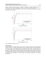
Fig. 11. Measured and Kriging predicted consumption [g/kWh] with ± 10% error bands
The emulator model is fitted to each response in turn and the RMSE, percentage RMSE are
recorded. These results are presented in Table3. The percentage RMSE results show that the
model has a %RMSE less than 4% of the range of the response data. This indicates roughly,
that if the emulator is used to predict the response at a new input setting, the error of
prediction can be expected to be less than 4%, when compared with the true value.
NOx Consumption
RMSE 40.51 19.99
%RMSE 2.45 3.04
Table 3. Kriging RMSE end %RMSE for each response: second approach case
6. Comparison and discussion
We recall that in the section 4, we have presented two different approaches, based on the
Kriging model. In this section we will try to make a comparison between these two
approaches, and discuss the advantages and inconvenient of each of them.
Case of NOx:
A legitimate question, which we could ask in the case of the estimate of NOx, is the
following one:
Why do we obtain a variogram of power type in the second approach, while we had
obtained a Gaussian variogram in the first approach, and the pressure is obtained with the
same parameters of control?
In fact, the power variogram obtained in the second approach is a better representation of
the true behavior of the emissions of NOx. Indeed, the interpretation of the power
variogram suggests that the variability of the response increases with the distance between
TwostageapproachesformodelingpollutantemissionofdieselenginebasedonKrigingmodel 43
We just notice that in the second approach, the accuracy of the predictions is improved for
the two responses, compared to the first approach. This improvement is very clear for the
consumption estimation.
We can explain this improvement, by the fact that in the second approach, we include
thermodynamic quantities such as the pressure, for the prediction of the two responses. The
inclusion of these quantities allows to bring back an additional knowledge for the prediction
of the both responses. Indeed, this knowledge results from the fact, that these quantities
represent the states variables of our system, and they characterize the behavior of
combustion in the internal of the combustion chamber.
Fig. 10. Measured and Kriging predicted NOx [ppm] with ± 10% error bands
Fig. 11. Measured and Kriging predicted consumption [g/kWh] with ± 10% error bands
The emulator model is fitted to each response in turn and the RMSE, percentage RMSE are
recorded. These results are presented in Table3. The percentage RMSE results show that the
model has a %RMSE less than 4% of the range of the response data. This indicates roughly,
that if the emulator is used to predict the response at a new input setting, the error of
prediction can be expected to be less than 4%, when compared with the true value.
NOx Consumption
RMSE 40.51 19.99
%RMSE 2.45 3.04
Table 3. Kriging RMSE end %RMSE for each response: second approach case
6. Comparison and discussion
We recall that in the section 4, we have presented two different approaches, based on the
Kriging model. In this section we will try to make a comparison between these two
approaches, and discuss the advantages and inconvenient of each of them.
Case of NOx:
A legitimate question, which we could ask in the case of the estimate of NOx, is the
following one:
Why do we obtain a variogram of power type in the second approach, while we had
obtained a Gaussian variogram in the first approach, and the pressure is obtained with the
same parameters of control?
In fact, the power variogram obtained in the second approach is a better representation of
the true behavior of the emissions of NOx. Indeed, the interpretation of the power
variogram suggests that the variability of the response increases with the distance between
AUTOMATION&CONTROL-TheoryandPractice44
the points. This interpretation joins the opinion of the experts, who say that for two various
engine configurations, the quantity of the corresponding NOx emissions will be also
different.
Obtaining a Gaussian variogram in the first approach, is explained by the fact that the speed
parameter of the engine take a raised values compared to the other control parameters. For
example, if we take the first and the second line of the table 5, which correspond to two
different engine speeds, we notice that the behavior of NOx is similar. However, the
distance between these two points, is very tall (caused by the engine speed) which explains
the sill on the variogram of the first approach.
Fortunately, this change in the behavior of variogram does not have an influence on the
prediction of NOx. But the interpretation of the variogram in the first approach can lead us
to make false conclusions. Indeed, in the case of the first approach, the variogram makes us
believe that the quantity of the NOx emissions remains invariant when we consider very
different configurations of control parameters. This does not reflect reality. In the case,
where we wish to use the variogram, to understand how a response varies. We advise to
check the values of the data, or to standardize the factors of the model.
N Prail Main
Mpil1
Mpil2
Pmain
Ppil1
Ppil2
VNT
VEGR
Volet NOx
1000 407,7 5,9
1,0
1,0
-4,4
-18,7
-11,2
79,9
36,0
75,9 67,0
2000 609,0 11,1 1,1 1,3 -5,9 -36,2 -15,2 67,4 34,5 75,9 64,1
Table5. Example of control parameters configuration
Case of consumption:
To manage to highlight the contribution of the second approach in the improvement of the
prediction of consumption we consider another representation of the results in figure 12.
We note that for the first approach, the Kriging method could estimate with a good accuracy
all the points which are close to the cloud used for the adjustment. The prediction of the
points which are far from the cloud was bad (as it is explained in section 5.1).
The use of the second approach brought back an improvement for the estimate of these
points. This gives a force of extrapolation to the Kriging method.
Fig. 12. Comparison of consumption estimation for the two case approaches. (the + points
are the experimental data and the red line is the model )
7. Conclusion
This paper deals with the problem of engine calibration, when the number of parameters of
control is considerable. An effective process to resolve such problems contains generally,
three successive stages: design of experiments, statistical modeling and optimization. In this
paper, we concentrate on the second stage. We discuss the important role of the
experimental design on the quality of the prediction of the Kriging model in the case of
consumption response. The Kriging model was adapted to allow an estimation of the
response in the case of higher dimensions. It was applied to predict the two engine
responses NOx and consumption through two approaches. The first approach gives
acceptable results. These results were clearly improved in the second approach especially in
the case of consumption. We demonstrate that the resulting model can be used to predict the
different responses of engine. It is easy to generalize for various diesel engine configurations
and is also suitable for real time simulations. In the future, this model will be coupled with
the evolutionary algorithms for multi-objective constrained optimization of calibration.
8. References
Arnaud, M.; Emery, X. (2000). Estimation et interpolation spatiale. Hermes Science
Publications, Paris.
Bates, R.A.; Buck, R.J.; Riccomagno, E. ; Wynn, H.P. (1996). Experimental Design and
Observation for large Systems. J. R. Statist. Soc. B, vol. 58, (1996) pp. 77-94.
Baillargeon, S.; Pouliot, J.; Rivest, L.P.; Fortin, V. ; Fitzback, J. interpolation statistique
multivariable de données de précipitations dans un cadre de modélisation
hydrologique, Colloque Géomatique 2004: un choix stratégique, Montréal (2004)
Castric, S.; Talon, V.; Cherfi, Z.; Boudaoud, N.; Schimmerling, N. P. A, (2007) Diesel engine
com-bustion model for tuning process and a calibration method. IMSM07 The
The second
a
pp
roach
The first
a
pp
roach
TwostageapproachesformodelingpollutantemissionofdieselenginebasedonKrigingmodel 45
the points. This interpretation joins the opinion of the experts, who say that for two various
engine configurations, the quantity of the corresponding NOx emissions will be also
different.
Obtaining a Gaussian variogram in the first approach, is explained by the fact that the speed
parameter of the engine take a raised values compared to the other control parameters. For
example, if we take the first and the second line of the table 5, which correspond to two
different engine speeds, we notice that the behavior of NOx is similar. However, the
distance between these two points, is very tall (caused by the engine speed) which explains
the sill on the variogram of the first approach.
Fortunately, this change in the behavior of variogram does not have an influence on the
prediction of NOx. But the interpretation of the variogram in the first approach can lead us
to make false conclusions. Indeed, in the case of the first approach, the variogram makes us
believe that the quantity of the NOx emissions remains invariant when we consider very
different configurations of control parameters. This does not reflect reality. In the case,
where we wish to use the variogram, to understand how a response varies. We advise to
check the values of the data, or to standardize the factors of the model.
N Prail Main
Mpil1
Mpil2
Pmain
Ppil1
Ppil2
VNT
VEGR
Volet NOx
1000 407,7 5,9
1,0
1,0
-4,4
-18,7
-11,2
79,9
36,0
75,9 67,0
2000 609,0 11,1
1,1
1,3
-5,9
-36,2
-15,2
67,4
34,5
75,9 64,1
Table5. Example of control parameters configuration
Case of consumption:
To manage to highlight the contribution of the second approach in the improvement of the
prediction of consumption we consider another representation of the results in figure 12.
We note that for the first approach, the Kriging method could estimate with a good accuracy
all the points which are close to the cloud used for the adjustment. The prediction of the
points which are far from the cloud was bad (as it is explained in section 5.1).
The use of the second approach brought back an improvement for the estimate of these
points. This gives a force of extrapolation to the Kriging method.
Fig. 12. Comparison of consumption estimation for the two case approaches. (the + points
are the experimental data and the red line is the model )
7. Conclusion
This paper deals with the problem of engine calibration, when the number of parameters of
control is considerable. An effective process to resolve such problems contains generally,
three successive stages: design of experiments, statistical modeling and optimization. In this
paper, we concentrate on the second stage. We discuss the important role of the
experimental design on the quality of the prediction of the Kriging model in the case of
consumption response. The Kriging model was adapted to allow an estimation of the
response in the case of higher dimensions. It was applied to predict the two engine
responses NOx and consumption through two approaches. The first approach gives
acceptable results. These results were clearly improved in the second approach especially in
the case of consumption. We demonstrate that the resulting model can be used to predict the
different responses of engine. It is easy to generalize for various diesel engine configurations
and is also suitable for real time simulations. In the future, this model will be coupled with
the evolutionary algorithms for multi-objective constrained optimization of calibration.
8. References
Arnaud, M.; Emery, X. (2000). Estimation et interpolation spatiale. Hermes Science
Publications, Paris.
Bates, R.A.; Buck, R.J.; Riccomagno, E. ; Wynn, H.P. (1996). Experimental Design and
Observation for large Systems. J. R. Statist. Soc. B, vol. 58, (1996) pp. 77-94.
Baillargeon, S.; Pouliot, J.; Rivest, L.P.; Fortin, V. ; Fitzback, J. interpolation statistique
multivariable de données de précipitations dans un cadre de modélisation
hydrologique, Colloque Géomatique 2004: un choix stratégique, Montréal (2004)
Castric, S.; Talon, V.; Cherfi, Z.; Boudaoud, N.; Schimmerling, N. P. A, (2007) Diesel engine
com-bustion model for tuning process and a calibration method. IMSM07 The
The second
a
pp
roach
The first
a
pp
roach
AUTOMATION&CONTROL-TheoryandPractice46
Third International Conference on Advances in Vehicul Control and Safety
AVCS'07, Buenos Aires, Argentine (2007).
Castric, S. (2007) Readjusting methods for models and application for diesel emissions, PhD
thesis, University of Technology of Compiègne, 2007.
Christakos, G. (1984). On the problem of permissible covariance and variogram models.
Water Resources Research, 20(2):251-265.
Cochran, W. G.; Cox, G. M. (1957). Experimental Designs. Second edition. New York : Wiley.
p 611.
Cressie, N. A. C. (1993) Statistics for spatial data. Wiley Series in Probability and
Mathematical Statistics: Applied Probability and Statistics. John Wiley & Sons Inc.,
New York. Revised reprint of the 1991 edition. A Wiley-Interscience Publication.
Davis, J.C. Statistics and Data Analysis in Geology, second edition John Wiley and Sons.
New York (1986).
Edwards,S.P.; A.D.P.; Michon, S.; Fournier, G. The optimization of common rail FIE
equipped engines through the use of statistical experimental design, mathematical
modelling and genetic algorithms, S.A.E paper, vol. 106, n
o
3, (1997), pp. 505-523.
Goers, A.; Mosher, L.; Higgins, B. (2003). Calibration of an aftermarket EFI conversion
system for increased performance and fuel economy with reduced emissions, S.A.E.
paper, vol. 112, n
o
3, March 2003, pp. 1390-1407, 2003-01-1051.
Heywood,J. (1988) Internal combustion engine fundamentals, London : Mac Graw-Hill
(1988)
Koehler J.R.; Owen A.B.(1996) Computer Experiments. In Ghosh, S., Rao, C.R.,(Eds.),
Handbook of Statistics, 13 : Designs and Analysis of Experiments, North- Holland,
Amsterdam, p.261-308. (1996)
Krige, D.G. (1951) A statistical approach to some basic mine valuation problems on the
Witwatersrand, J. of Chem. Metal. and Mining Soc. of South Africa. Vol. 52 pp 119-139
(1951).
McKay M.D., Beckman R.J., Conover W.J. Comparison of three methods for selecting values
input variables in the analysis of output from a computer code, Technometrics, Vol.
42, n
o
1, (February 2000) pp. 55 – 61, 239-245
Matheron, G. (1963) Principles of Geostatistics, Economic Geology, v. 58, n
o
8, (December
1963) pp. 1246-12688.
Pierpont D. A.; Montgomery D. T.; Reitz R. D. Reducing particulate and NOx using multiple
injection and EGR in a D.I. diesel, S.A.E paper, vol. 104, n
o
4 March(1995) , pp. 171-
183 950217.
Pilley, A.D.; A.J.B.; Robinson, D.; Mowll, D. (1994) Design of experiments for optimization of
engines to meet future emissions target, International Symposium on Advanced
Transportation Applications (1994).
Sacks J., Schiller S.B., Welch W.J. (1989) Designs for Computer Experiments. Technometrics,
vol. 31,41-47.
Schimmerling, P.; J.C.S. ; Zaidi, A. (1998) Use of design of experiments. Lavoisier.
Stein, M. Large sample properties of simulations using Latin hypercube sampling,
Technometrics, vol. 29, n
o
2, (1987) pp. 143-151, 0040-1706.
AnapproachtoobtainaPLCprogramfromaDEVSmodel 47
AnapproachtoobtainaPLCprogramfromaDEVSmodel
HyeongT.Park,KilY.Seong,SurajDangol,GiN.WangandSangC.Park
X
An approach to obtain a PLC
program from a DEVS model
Hyeong T. Park, Kil Y. Seong, Suraj Dangol,
Gi N. Wang and Sang C. Park
Department of Industrial Information & System Engineering, Ajou University
Republic of Korea
1. Introduction
To survive and prosper in the modern manufacturing era, a manufacturing company should
be capable of adapting reduced life cycle of products in a continuously changing market place.
Simulation is a useful tool for manufacturers to adapt this kind of rapidly changing market to
design and analyze complex systems that are difficult to model analytically or mathematically
(Choi, 2000). Manufacturers who are using simulation can reduce time to reach stable state of
automated manufacturing process by utilizing statistics, finding bottlenecks, pointing out
scheduling error etc. For the simulation of manufacturing systems, manufacturers have been
using various simulation languages, simulation software for example ARENA, AutoMod.
Most of traditional simulation languages and softwares focus on the representation of
independent entity flows between processes; their method is commonly referenced to as a
transaction-oriented approach. In this paper, we propose an object-oriented approach that is
based on the set of object classes capable of modeling a behavior of existing system
components.
The object-oriented modeling (OOM) is a modeling paradigm, that uses real world objects for
modeling and builds language independent design organized around those objects
(Rumbaugh, 1991). Even though OOM has been widely known to be an effective method for
modeling complicated software systems, very few researchers tried to apply the OOM to
design and simulate manufacturing system software models. Based on the OOM paradigm,
different researchers have proposed various modeling approaches despite the fact that they
express them in different ways with different notations. For example, Choi et al. presented the
JR-net framework for modeling which is based on the OOM paradigm of Rumbaugh et al.,
which is made of three sub-models(an object model, functional model, and dynamic model).
Chen and Lu proposed an object-oriented modeling methodology to model production
systems in terms of the Petri-nets, the entity relationship diagram (ERD) and the IDEF0 (Chen,
1994). Virtual factory (VF) is also very important concept to be considered in today’s
simulation environment. By using the OOM paradigm, VF concept can be implemented
efficiently (Onosato, 1993).
Recently, Park (Park, 2005) proposed a ‘three-phase-modeling framework’ for creating a
virtual model for an automated manufacturing system. This paper employs the three-phase-
4
AUTOMATION&CONTROL-TheoryandPractice48
modeling framework of creating a virtual model, and the Discrete Event System
Specification(DEVS) (Zeigler, 1984) for process modeling. The proposed virtual model consists
of four types of objects. The virtual device model represents the static layout of devices. This
can be decomposed into the shell and core, which encourages the reusability making possible
to adapt different system configurations. For the fidelity of the virtual model, The Transfer
handler model handles a set of device-level command that mimics the physical mechanism of
a transfer. The Flow controller model decides the firable transfers based on decision variables
that are determined by the State manager model. The State manager model and Flow
controller model can be converted to PLC part. After finishing the process modeling by
employing the three-phase-modeling framework, those two models will be the control
information for the converting to PLC.
The overall structure of the paper is as follows. Section 2 represents the brief explanation about
the PLC, and Section 3 is about the DEVS. The overall approach to create manufacturing
system model for generation PLC code is described in Section 4. Section 5 gives as example cell,
which is observed to find correlation between the PLC code and the DEVS model in Section 6.
Finally, Conclusion and discussion is addressed in Section 7.
2. Programmable Logic Controller(PLC)
The Programmable Logic Controller (PLC) is an industrial computer used to control
automated processes in manufacturing (Parr, 1999). PLC is designed for multiple inputs and
outputs arrangements, it detects process state data through the sensing devices such as limit
sensors, proximity sensors or signals from the robots executes logics in its memory and
triggers the next command through the actuator such as motor, solenoid valve or command
signal for the robots etc. PLC executes the control logic programmed in different types of
languages. IEC published IEC 61131-3 to standardize PLC languages including Ladder
diagram, Sequential Function Chart, Structured Text and Function Block Diagram (Maslar,
1996).
Fig. 1. The PLC code in the form of Ladder diagram
3. Discrete Event System Specification(DEVS)
DEVS formalism is introduced by Zeigler, which is a theoretic formalism and it supplies a
means of modeling discrete event system in a modular, hierarchical way. With this DEVS
formalism, we can perform modeling more easily and correctly by dividing large system
into segment models and define the coupling between them. Formally, an atomic model M
is specified by a 7-tuple:
M = < X, S, Y, δ
int,
δ
ext,
λ, t
a
>
X : input events set;
S : sequential states set;
Y : output events set;
δ
int
: SS : internal transition function;
δ
ext
: Q x X S : external transition function
Q = { (s, e)|s ∈ S, 0 ≤ e ≤t
a
(s)}
: total state of M;
λ: S->Y : output function;
t
a
: S
Real : time advance function:
The second form of the model, called a coupled model, indicates how to couple several
element models together to form a new and bigger model. Formally, a coupled model DN is
defined as:
DN = < X, Y, M, EIC, EOC, IC, SELECT >
X : input events set;
Y : output events set;
M: set of all component models in DEVS;
EIC ∈ DN.IN x M.IN : external input coupling relation;
EOC ∈ M.OUT x DN.OUT : external output coupling relation;
AnapproachtoobtainaPLCprogramfromaDEVSmodel 49
modeling framework of creating a virtual model, and the Discrete Event System
Specification(DEVS) (Zeigler, 1984) for process modeling. The proposed virtual model consists
of four types of objects. The virtual device model represents the static layout of devices. This
can be decomposed into the shell and core, which encourages the reusability making possible
to adapt different system configurations. For the fidelity of the virtual model, The Transfer
handler model handles a set of device-level command that mimics the physical mechanism of
a transfer. The Flow controller model decides the firable transfers based on decision variables
that are determined by the State manager model. The State manager model and Flow
controller model can be converted to PLC part. After finishing the process modeling by
employing the three-phase-modeling framework, those two models will be the control
information for the converting to PLC.
The overall structure of the paper is as follows. Section 2 represents the brief explanation about
the PLC, and Section 3 is about the DEVS. The overall approach to create manufacturing
system model for generation PLC code is described in Section 4. Section 5 gives as example cell,
which is observed to find correlation between the PLC code and the DEVS model in Section 6.
Finally, Conclusion and discussion is addressed in Section 7.
2. Programmable Logic Controller(PLC)
The Programmable Logic Controller (PLC) is an industrial computer used to control
automated processes in manufacturing (Parr, 1999). PLC is designed for multiple inputs and
outputs arrangements, it detects process state data through the sensing devices such as limit
sensors, proximity sensors or signals from the robots executes logics in its memory and
triggers the next command through the actuator such as motor, solenoid valve or command
signal for the robots etc. PLC executes the control logic programmed in different types of
languages. IEC published IEC 61131-3 to standardize PLC languages including Ladder
diagram, Sequential Function Chart, Structured Text and Function Block Diagram (Maslar,
1996).
Fig. 1. The PLC code in the form of Ladder diagram
3. Discrete Event System Specification(DEVS)
DEVS formalism is introduced by Zeigler, which is a theoretic formalism and it supplies a
means of modeling discrete event system in a modular, hierarchical way. With this DEVS
formalism, we can perform modeling more easily and correctly by dividing large system
into segment models and define the coupling between them. Formally, an atomic model M
is specified by a 7-tuple:
M = < X, S, Y, δ
int,
δ
ext,
λ, t
a
>
X : input events set;
S : sequential states set;
Y : output events set;
δ
int
: SS : internal transition function;
δ
ext
: Q x X S : external transition function
Q = { (s, e)|s ∈ S, 0 ≤ e ≤t
a
(s)}
: total state of M;
λ: S->Y : output function;
t
a
: S
Real : time advance function:
The second form of the model, called a coupled model, indicates how to couple several
element models together to form a new and bigger model. Formally, a coupled model DN is
defined as:
DN = < X, Y, M, EIC, EOC, IC, SELECT >
X : input events set;
Y : output events set;
M: set of all component models in DEVS;
EIC ∈ DN.IN x M.IN : external input coupling relation;
EOC ∈ M.OUT x DN.OUT : external output coupling relation;
AUTOMATION&CONTROL-TheoryandPractice50
IC ∈ M.OUT x M.IN : internal coupling relation;
SELECT : 2
M
- ø-> M : tie-breaking selector,
Where the extension .IN and .OUT represent the input ports set and the output ports set of
each DEVS models.
4. Approach to create manufacturing system model to generate PLC code
To construct the automated process, the factory designers have to consider the overall
process layout. After deciding skeletal layout, the process cycle time is simulated by the
discrete event system software like ARENA or AutoMod. In this stage, including the process
cycle time and production capability, the physical validity and efficiency of co-working
machines are also described. Simulation and modeling software QUEST or IGRIP are used
for this purpose (Breuss, 2005).
Fig. 2. Automated factory construction procedure
On the next step, the PLC code programming for logical functioning is done without
utilizing information from previous discrete event systems modeling. The gap between the
high level simulation of discrete event system and the low level physical process control
logic need to be bridged for the utilization of process modeling and practical simulation in
terms of physical automated device movement. This paper tries to find the bridge between
these two different simulation levels and further describes automatic generation of PLC
code from the DEVS model.
In developing the DEVS model, the first thing we have to do is to model the manufacturing
system by the three-phase-modeling framework ( Park, 2005). The framework describes
manufacturing system modeling with 4 components; the Virtual device model, the Transfer
handler model, the State manager model and the Flow controller model as shown in Figure
3.
Fig. 3. Outline of the virtual manufacturing model
The Virtual device model shows the manufacturing devices. It has input port to receive the
action signal and output port to send the work done signal. The Transfer handler model
handles the parts stream and assisting resources (tools and pallets) between devices. This
approach focused on the physical mechanism enabling the transfer than conventional
approaches. In reality, a transfer happens by the combination of device-level command
between co-working devices (giving and taking devices). The State manager model collects
the state data of every device. Whenever there is a state change of devices, it will update the
device states. Then, this information will be delivered to the Flow controller model as a
decision variable. After getting the state information from the State manager model, the
Flow controller model will decide firable transfer based on the system state (decision
variables).
For the implementation of the virtual manufacturing system model, this paper employs the
Discrete Event Systems Specification (DEVS) formalism, which supports the specification of
discrete event models in a hierarchical modular manner. The formalism is highly compatible
with OOM for simulation. Under the DEVS formalism, we need to specify two types of sub-
models: (1) the atomic model, the basic models, from which larger ones are built and (2) the
coupled model, how atomic models are related in a hierarchical manner.
AnapproachtoobtainaPLCprogramfromaDEVSmodel 51
IC ∈ M.OUT x M.IN : internal coupling relation;
SELECT : 2
M
- ø-> M : tie-breaking selector,
Where the extension .IN and .OUT represent the input ports set and the output ports set of
each DEVS models.
4. Approach to create manufacturing system model to generate PLC code
To construct the automated process, the factory designers have to consider the overall
process layout. After deciding skeletal layout, the process cycle time is simulated by the
discrete event system software like ARENA or AutoMod. In this stage, including the process
cycle time and production capability, the physical validity and efficiency of co-working
machines are also described. Simulation and modeling software QUEST or IGRIP are used
for this purpose (Breuss, 2005).
Fig. 2. Automated factory construction procedure
On the next step, the PLC code programming for logical functioning is done without
utilizing information from previous discrete event systems modeling. The gap between the
high level simulation of discrete event system and the low level physical process control
logic need to be bridged for the utilization of process modeling and practical simulation in
terms of physical automated device movement. This paper tries to find the bridge between
these two different simulation levels and further describes automatic generation of PLC
code from the DEVS model.
In developing the DEVS model, the first thing we have to do is to model the manufacturing
system by the three-phase-modeling framework ( Park, 2005). The framework describes
manufacturing system modeling with 4 components; the Virtual device model, the Transfer
handler model, the State manager model and the Flow controller model as shown in Figure
3.
Fig. 3. Outline of the virtual manufacturing model
The Virtual device model shows the manufacturing devices. It has input port to receive the
action signal and output port to send the work done signal. The Transfer handler model
handles the parts stream and assisting resources (tools and pallets) between devices. This
approach focused on the physical mechanism enabling the transfer than conventional
approaches. In reality, a transfer happens by the combination of device-level command
between co-working devices (giving and taking devices). The State manager model collects
the state data of every device. Whenever there is a state change of devices, it will update the
device states. Then, this information will be delivered to the Flow controller model as a
decision variable. After getting the state information from the State manager model, the
Flow controller model will decide firable transfer based on the system state (decision
variables).
For the implementation of the virtual manufacturing system model, this paper employs the
Discrete Event Systems Specification (DEVS) formalism, which supports the specification of
discrete event models in a hierarchical modular manner. The formalism is highly compatible
with OOM for simulation. Under the DEVS formalism, we need to specify two types of sub-
models: (1) the atomic model, the basic models, from which larger ones are built and (2) the
coupled model, how atomic models are related in a hierarchical manner.
AUTOMATION&CONTROL-TheoryandPractice52
When the DEVS model is developed, both the State manager atomic model for the process
monitoring and the Flow controller atomic model for the actual control can be replaced the
PLC part. Namely, control part for the manufacturing cell. Here is the goal of this paper.
5. DEVS modelling of a simple cell based on the three-phase-modeling
framework
In this Chapter, we will observe a small work cell example. The work cell is modeled
according to the three-phase-modeling framework and converted to the DEVS model like
mentioned above. Finally, we will compare the DEVS model and the PLC code to find some
meaningful bridge.
Figure 4 shows the small cell example. At first, an entity is generated from the Stack, which
will lay on the AGV machine in P1, then AGV senses this raw part and moves to the P2 for
machining. When machine detects the part arrival by the AGV, the machine starts to
operate.
Fig. 4. Example cell
When we consider this example cell in terms of the three-phase-modeling framework, there
are three virtual device models; the stack model, the AGV model and the machine model.
The stack model generates the raw part entity and places it on the AGV for transfer. Until
this point, the entity transfer process is between the stack and the AGV virtual device model
as a result the transfer handler model is created between the stack the AGV model.
Similarly, entity transferring between the AGV model and the Machine happens. This
transfer handling model can be represented as THam. If there is any state change among the
virtual devices, the changes are supposed to be reported to the State manager model. The
State manager model maintains the decision variables in compliance with the reported state
changes of the virtual devices and the Flow controller model will make a decision on firable
transfer based on the decision variables. Figure 5 represents the constructed model about the
example cell.
Fig. 5. Modeling of the example cell in the Park’s methodology
Once the modeling by means of the three-phase-modeling framework is finished, second
step is to convert the model to the DEVS formalism. In this example, every model is
converted to the atomic model and entire cell will be the coupled model that is consist of all
atomic models. Figure 6 is the converted DEVS model example of AGV. In the traditional
implementation of discrete event system simulation using DEVS, DEVSIM++ is a simulation
framework which realizes the DEVS formalism for modeling and related abstract simulator
concepts for simulation, all in C++ (Kim, 1994). Through this open source frame, we can
develop the discrete event system simulation engine easily. Once, both the DEVS
implementation and the simulation with PLC control logic is done, we can achieve the
overall physical control simulator for automated process.
AnapproachtoobtainaPLCprogramfromaDEVSmodel 53
When the DEVS model is developed, both the State manager atomic model for the process
monitoring and the Flow controller atomic model for the actual control can be replaced the
PLC part. Namely, control part for the manufacturing cell. Here is the goal of this paper.
5. DEVS modelling of a simple cell based on the three-phase-modeling
framework
In this Chapter, we will observe a small work cell example. The work cell is modeled
according to the three-phase-modeling framework and converted to the DEVS model like
mentioned above. Finally, we will compare the DEVS model and the PLC code to find some
meaningful bridge.
Figure 4 shows the small cell example. At first, an entity is generated from the Stack, which
will lay on the AGV machine in P1, then AGV senses this raw part and moves to the P2 for
machining. When machine detects the part arrival by the AGV, the machine starts to
operate.
Fig. 4. Example cell
When we consider this example cell in terms of the three-phase-modeling framework, there
are three virtual device models; the stack model, the AGV model and the machine model.
The stack model generates the raw part entity and places it on the AGV for transfer. Until
this point, the entity transfer process is between the stack and the AGV virtual device model
as a result the transfer handler model is created between the stack the AGV model.
Similarly, entity transferring between the AGV model and the Machine happens. This
transfer handling model can be represented as THam. If there is any state change among the
virtual devices, the changes are supposed to be reported to the State manager model. The
State manager model maintains the decision variables in compliance with the reported state
changes of the virtual devices and the Flow controller model will make a decision on firable
transfer based on the decision variables. Figure 5 represents the constructed model about the
example cell.
Fig. 5. Modeling of the example cell in the Park’s methodology
Once the modeling by means of the three-phase-modeling framework is finished, second
step is to convert the model to the DEVS formalism. In this example, every model is
converted to the atomic model and entire cell will be the coupled model that is consist of all
atomic models. Figure 6 is the converted DEVS model example of AGV. In the traditional
implementation of discrete event system simulation using DEVS, DEVSIM++ is a simulation
framework which realizes the DEVS formalism for modeling and related abstract simulator
concepts for simulation, all in C++ (Kim, 1994). Through this open source frame, we can
develop the discrete event system simulation engine easily. Once, both the DEVS
implementation and the simulation with PLC control logic is done, we can achieve the
overall physical control simulator for automated process.
AUTOMATION&CONTROL-TheoryandPractice54
Fig. 6. DEVS model of the AGV
6. Correlation between the PLC code and the DEVS models
For the auto generation of PLC code from the DEVS model, we need to examine the PLC
code of example cell and the DEVS models, especially the State manager and the Flow
controller model.
In the manufacturing unit, PLC collects the process state information through the sensors.
These sensor signals are referenced to decide next command or operation. This task is done
by the state manager model in the modeled frame. The State manager model detects every
change in state of the virtual device and then updates the decision variables. Similar to PLC
code, the Flow controller model is supposed to have running logic that is kind of
combination of decision variables. As a result, PLC code from the DEVS model can be
divided into two parts. One part is for updating the decision variable from the signal of
input port in the State manager model. Another is for actual logic composed of decision
variables to fulfill the intended process control.
Fig. 7. Two part of PLC code
In the front part, the State manager model collects every state changes through the input
port. The one input port of example cell has different kind of signal depend on the state. For
example, the input port I2 is the signal from the AGV and it has 4 different kinds of state
signals. With the same way, each input port of the State manager model has multiple input
signals like shown in Table 1.
Atomic
models
States Input Signals
I1 Stack
Idle,
Release
STACK_IDLE
STACK_RELEASE
I2 AGV
P1,
GoP2,
P2,
GoP1
AGV_P1
AGV_GOP2
AGV_P2
AGV_GOP1
I3 Machine
Idle,
Run
MACHINE_IDLE
MACHINE_RUN
Table 1. The States of Atomic models
The memory structure in the PLC code can be classified into three groups. The first group is
input memory which consists of input signal names and the second group is the output
memory consisting output signal names and the last is the internal memory which is used to
maintain the signal information of input or output and for temporary numerical calculation.
AnapproachtoobtainaPLCprogramfromaDEVSmodel 55
Fig. 6. DEVS model of the AGV
6. Correlation between the PLC code and the DEVS models
For the auto generation of PLC code from the DEVS model, we need to examine the PLC
code of example cell and the DEVS models, especially the State manager and the Flow
controller model.
In the manufacturing unit, PLC collects the process state information through the sensors.
These sensor signals are referenced to decide next command or operation. This task is done
by the state manager model in the modeled frame. The State manager model detects every
change in state of the virtual device and then updates the decision variables. Similar to PLC
code, the Flow controller model is supposed to have running logic that is kind of
combination of decision variables. As a result, PLC code from the DEVS model can be
divided into two parts. One part is for updating the decision variable from the signal of
input port in the State manager model. Another is for actual logic composed of decision
variables to fulfill the intended process control.
Fig. 7. Two part of PLC code
In the front part, the State manager model collects every state changes through the input
port. The one input port of example cell has different kind of signal depend on the state. For
example, the input port I2 is the signal from the AGV and it has 4 different kinds of state
signals. With the same way, each input port of the State manager model has multiple input
signals like shown in Table 1.
Atomic
models
States Input Signals
I1 Stack
Idle,
Release
STACK_IDLE
STACK_RELEASE
I2 AGV
P1,
GoP2,
P2,
GoP1
AGV_P1
AGV_GOP2
AGV_P2
AGV_GOP1
I3 Machine
Idle,
Run
MACHINE_IDLE
MACHINE_RUN
Table 1. The States of Atomic models
The memory structure in the PLC code can be classified into three groups. The first group is
input memory which consists of input signal names and the second group is the output
memory consisting output signal names and the last is the internal memory which is used to
maintain the signal information of input or output and for temporary numerical calculation.
AUTOMATION&CONTROL-TheoryandPractice56
The name of input signal can be determined with combination between the input port and
its state name. In this way, we can give a name to all input signals.
As mentioned before, the flow controller model reads the decision variables to execute next
command. Thus, we have to make decision variables representing the process state as the
internal memory. As we did in the input variable for naming, we can give decision
variables’ name by putting the ‘On’ between the port name and the state name. Then, this
decision variable shows the port’s current state is active condition. Once decision variables
are set, the Flow controller detects the firable output signals from the set variables. Figure 8
show the decision variables of each input of AGV model and moving condition. To the
AGV, the possible condition to move from P1 to P2 is when the raw part is on the AGV,
AGV’s state is ‘GoP2’, and the machine state is ‘Idle’ at the same time.
Fig. 8. The triggering condition for AGV move
As we have noticed for the case of the AGV model, the other devices’ executing condition
can be derived. While the PLC code for the State manager model part can be generated
automatically with a combination of decision variables, the flow controller part is sometimes
rather ambiguous. That is because unlike the flow controller, DEVS model is quite abstract
and high level, the PLC part is very specific control area. Even though, process system
designer can construct the DEVS model including low level of PLC, normally DEVS
modeling is not fulfilled in this way. This aspect will be limitation or designer’s choice in
reference to PLC code auto generation. The DEVS modeling here is done specifically in
mind of the PLC code generation of the Flow Controller model part. Figure 9 illustrates the
two part of PLC code about the AGV from the State manager and the Flow controller model.
And the Flow controller DEVS model for PLC code auto generation with the simple work
cell is shown in Fig. 10.
7. Discussion and conclusion
This paper presents the PLC code auto generation methodology from the DEVS model. The
PLC level control logic is rather closed and unopened engineering area while discrete event
system modeling and simulation is widely used to measure the process capacity. By using
the discrete event system simulation technique, the process or overall cycle time and
throughput can be calculated.
Fig. 9. PLC code from the State Manager and the Flow Controller model
Fig. 10. The Flow Controller DEVS model
AnapproachtoobtainaPLCprogramfromaDEVSmodel 57
The name of input signal can be determined with combination between the input port and
its state name. In this way, we can give a name to all input signals.
As mentioned before, the flow controller model reads the decision variables to execute next
command. Thus, we have to make decision variables representing the process state as the
internal memory. As we did in the input variable for naming, we can give decision
variables’ name by putting the ‘On’ between the port name and the state name. Then, this
decision variable shows the port’s current state is active condition. Once decision variables
are set, the Flow controller detects the firable output signals from the set variables. Figure 8
show the decision variables of each input of AGV model and moving condition. To the
AGV, the possible condition to move from P1 to P2 is when the raw part is on the AGV,
AGV’s state is ‘GoP2’, and the machine state is ‘Idle’ at the same time.
Fig. 8. The triggering condition for AGV move
As we have noticed for the case of the AGV model, the other devices’ executing condition
can be derived. While the PLC code for the State manager model part can be generated
automatically with a combination of decision variables, the flow controller part is sometimes
rather ambiguous. That is because unlike the flow controller, DEVS model is quite abstract
and high level, the PLC part is very specific control area. Even though, process system
designer can construct the DEVS model including low level of PLC, normally DEVS
modeling is not fulfilled in this way. This aspect will be limitation or designer’s choice in
reference to PLC code auto generation. The DEVS modeling here is done specifically in
mind of the PLC code generation of the Flow Controller model part. Figure 9 illustrates the
two part of PLC code about the AGV from the State manager and the Flow controller model.
And the Flow controller DEVS model for PLC code auto generation with the simple work
cell is shown in Fig. 10.
7. Discussion and conclusion
This paper presents the PLC code auto generation methodology from the DEVS model. The
PLC level control logic is rather closed and unopened engineering area while discrete event
system modeling and simulation is widely used to measure the process capacity. By using
the discrete event system simulation technique, the process or overall cycle time and
throughput can be calculated.
Fig. 9. PLC code from the State Manager and the Flow Controller model
Fig. 10. The Flow Controller DEVS model
AUTOMATION&CONTROL-TheoryandPractice58
However, there is a big gap between the PLC code and the discrete event system simulation.
This gap causes the repetition of process analysis work for the PLC programmer and the
time delay to implement automated processing system in a manufacturing unit.
The overall procedure for proposed approach has three steps. Modeling the real system
according to the three-phase-modeling framework is first step. And this model is converted
to the DEVS formalism in second step. Among the 4 kind of models, the State manger and
the Flow controller model is going to be replaced to the PLC part.
The generated PLC code from our approach can be categorized into two parts, one is from
the state manager and another is from the flow controller. The first part is created from the
input signals and the decision variable. And the latter part is from the control part which is
from combination of decision variables.
The latter part generation is not achieved perfectly because the DEVS modeling level is more
abstracted than the PLC level. However, this approach offers the overall framework for the
PLC code generation from DEVS model. In the following future, the direction mentioned
above will be the inevitable stream for the more physical process simulation, for the time
saving toward the mass production condition and for better competitiveness to the company.
8. References
B. K. Choi, B. H. Kim, 2000. Paper templates, In Current Advances in Mechanical Design and
Production Seventh Cairo University International MDP Conference. New Trend in
CIM: virtual manufacturing systems for next generation manufacturing.
J. Rumbaugh, M. Blaha, W. Premerlani. 1991. Paper templates, In Prentice Hall Inc. Object-
Oriented Modeling and Design.
B. K. Choi, H. Kwan, T. Y. Park, 1996. Paper templates, In The International journal of Flexible
Manufacturing Systems. Object-Oriendted graphical modelling of FMSs.
K. Y. Chen, S. S. Lu, 1997. Paper templates, In International journal of Computer Integrated
Manufacturing. A Petri-net and entity-relationship diagram based object oriented
design method for manufacturing systems control.
M. Onosato, K. Iwata, 1993. Paper templates, In CIRP. Development of a virtual
manufacturing system by integrating product models and factory models.
Sang C. Park, 2005. Paper templates, In Computers in Industry. A methodology for creating a
virtual model for a flexible manufacturing system.
B. P. Zeigler, 1984. Paper templates, In Academic Press. Multifacetted Modeling and Discrete
Event Simulation.
E. A. Parr, 1999. The book, Programmable Controllers : An Engineer’s Guide 3
rd
ed.
M. Maslar, 1996. Paper templates, In IEEE Pulp and Paper Industry Technical Conference. PLC
standard programming language: IEC61131-3
F. Breuss, W. Roeger, 2005. Paper templates, In Journal of Policy Modeling. The SGP fiscal
rule in the case of sluggish growth: Simulations with the QUEST
T. G. Kim, 1994. The Book. DEVS++ User’s Manual
Aframeworkforsimulatinghomecontrolnetworks 59
Aframeworkforsimulatinghomecontrolnetworks
Rafael J. Valdivieso-Sarabia, Jorge Azorín-López, Andrés Fuster-Guilló and Juan M.
García-Chamizo
X
A framework for simulating
home control networks
Rafael J. Valdivieso-Sarabia, Jorge Azorín-López,
Andrés Fuster-Guilló and Juan M. García-Chamizo
University of Alicante
Spain
1. Introduction
Trasgu
1
is a control networks design environment valid for digital home or other places. The
introduction of services provided by information society technologies, especially control
networks, is growing at business, buildings, houses… There are a high number of protocols
and technologies available in control networks. The set of control technologies that makes
the applications viable are diverse and each follows his own rules. For example, there are
different standard for control technologies like X10 (Fuster & Azorín, 2005), KNX/EIB
(Haenselmann et al., 2007), LonWorks (Ming et al., 2007) , CAN (Jung et al., 2005), Zigbee
(Pan & Tseng, 2007), etc and owned technologies like Bticino, Vantage, X2D, In spite of
standardization attempt, the design and implementation of control facilities is complex.
Every technology presents a few limitations. We find among them the own configuration
tool. It is proprietary software that allows the network design and configuration.
Proprietary software, provided by the supplier, is the main design and configuration tool for
control networks. Tools used by technologies considered as automation networks standard
are: European Installation Bus Tool Software (ETS) for Konnex (KNX), and LonMaker
Integration Tool (LonMaker) for Lonworks. Both tools have the same purpose, but they have
different design and configuration methodology. A design realized with any tool is not
compatible with other one and in many cases they cannot be linked. This has repercussions
on increase of time and cost when the design needs several technologies that must coexist to
offer a higher service. Technology choice depends of user requirements, because it might not
be solved as well with all technologies. Even there might be project whose requirements are
unsolved with a single technology, so we will need some technologies integration. In many
situations, it turns out complex to integrate them in a common system. In spite of it, we need
to communicate them to provide higher services, even if they belong to different networks:
control networks, information networks, multimedia networks and security networks. There
are residential gateways based on middleware and discovery protocols to make integration
task easier.
1
Trasgu is Asturian (Spanish) mythology goblin. It realizes household chores, but if it gets
angry, he will break and hide objects, he will shout, etc.
5
AUTOMATION&CONTROL-TheoryandPractice60
Residential gateway middleware is connectivity software that allows communication among
different technologies, in this case control technologies. Common middleware in ICT are:
CORBA, J2EE y .Net. J2EE and .Net are the most used, the first one is based on Java and the
second one is based on different Microsoft programming languages: C#, Java#, Visual Basic
.Net,
Discovery protocols facilitate devices connection to networks and services negotiation:
Universal Plug and Play (UPnP) (Rhee et al., 2004), Jini Network Technology (Sun, 1999),
Home Audio/Video Interoperability (Havi), Open Service Gateway initiative (OSGi)
(Kawamura & Maeomichi, 2004), Services and Network for Domotics Applications
(SENDA) (Moya & López, 2002) UPnP is an open architecture distributed on a network,
which is independent from technology. The goal is to get an unattended connection among
different devices technology. Jini gets infrastructure to federate services in a distributed
system. It is based on Java programming language. Jini has not been successful because
there are not many devices supporting Jini. Havi is architecture oriented to electrodomestic
appliance. The objective is to get a services set to make interoperability and distribuited
networks development in home easier. OSGi defines a open and scalable framework to
execute services in a safe way. The goal is to join devices in a heterogeneus network at
aplication layer in order to compone services. SENDA framework is a device networking
that uses CORBA. The aim of SENDA is similar to OSGi philosophy although SENDA is
trying to improve it. There are some technologies to integrate control network, but none of
them is being clearly succesful in all contexts, although some of them have a little market
share.
Independently from integration there is another problem in actual control networks. Once
we have designed a control network according to user requiments, we must realize the
network installation to validate the correct operation. This fact introduces high temporal
and economical costs in the installation, because if designer detects a fault, he should to
solve it in the real facilities. This situation can be avoided through a simulation task after
designing and before network installing, but control networks owned tools do not allow
realizing simulations. They manage to realize validations to low level. For example, ETS
realizes validations with physical and group addresses assigned to the devices. There is a
tool associated with the ETS called EIB Interworking Test Tool, EITT. It is specialized in
analysis of devices, moreover offers the possibility of simulating the network protocols. In
spite of the low level validations that these tools realize, none of them manages to realize a
simulation of the control network behaviour. A consequence is that designer cannot be able
to verify the correct functioning, until control network has been implemented and installed.
Simulation brings advantages in the design of control installation. Simulation as a tool in the
development techno-scientist allows detect errors prematurely in the design phase
(Denning, 1989). It is able to verify and validate the control network design (Balci, 1998) in
order to reduce costs. Simulation has the same place in design phase, that testing at
implementation phase, since in both cases checks are made on the work performed.
Therefore simulation is seen as a test case (Norton & Suppe, 2001), where checks are made to
a higher level of abstraction. Besides the professional tools, in the literature there are some
control network simulators like VINT project (Breslau, 2000), DOMOSIM (Bravo et al., 2000),
(Bravo et al., 2006), VISIR (González et al. 2001) and (Conte, 2007). The VINT project
presents a common simulator containing a large set of networks model. It is composed by a
simulator base and a visualization tool. It is focused for simulation of TCP/IP network
protocols for research in TCP behaviour, multicast transport, multimedia, protocols
response to topology changes, application level protocols, etc.
DOMOSIM and VISIR are orientated to educational area, so his principal use is teaching
methodology of design of facilities. The negative aspect is the disability to join with tools of
design that are used in the professional environment. (Conte, 2007) presents a study of
home automation systems through simulation/emulation environment. It modelling home
automation system like agents, where each agent action is characterized with cost, duration
and quality. The agent behaviour is modelled with a set of states and a set of rules. The
simulator is a software environment and agents are implemented in LabView and
LabWindows CVI and are executed at same time. To run a simulation, user has to define the
virtual environment and execute it. This is a powerful simulation environment but is not
integrated in designing environment, so we must design the control network in the owned
tool and later we must re-design at simulation environment.
Control networks carry a high temporary and economic cost. High cost due to three factors
principally: Requirements of integration different technologies, inappropriate designing
methodologies and design validation by means of experimentation. The proposal gathered
in this chapter is to provide an environment to provide control network architectures in the
digital home. The objective is that these architectures can be valid for any technology,
paying special attention to network simulation task.
2. Modelling control systems
Modelling systems are based principally in two types of methodologies: bottom-up
methodologies and top-down methodologies (Sommerville, 2004).
The technologies and methods used for the modelling of home automated systems are few
developed. They are based on the use of very low level technologies (Muñoz et al., 2004).
The great diversity of control technologies causes that designing control networks following
bottom-up methodologies might turn out a complex task and might generate systems
inadequate to requirements.
The top-down methodologies are characterized essentially abstract. They require that
ingenuities are conceived before any consideration. Ingenuities are conceived, therefore, free
from any condition imposed by the technologies. These methodologies match perfectly with
our philosophy of design independent implementation technologies.
Model Driven Architecture (MDA) (Mellor et al., 2004) and Services Oriented Architectures
(SOA) (Newcomer & Lomow, 2005) are within independent implementation philosophy. In
one hand MDA allows transitions from conceptual models of systems using automatic code
generation is possible to obtain fast and efficient middleware solutions. In the other hand
SOA provides a methodology and framework for documenting business skills and power to
support the consolidation and integration activities. The network nodes make its resources
available to other participants in the network as independent services that have access to a
standardized way. In contrast to object-oriented architectures, SOAs are formed by
application services weakly coupled and highly interoperable. The communication between
these services is based on a formal definition platform independent and programming
language. The interface definition’s encapsulates the peculiarities of an implementation,
which makes it independent of the technology, the programming language or developer.
Designing control networks, with this methodology, require answer the following questions:
Aframeworkforsimulatinghomecontrolnetworks 61
Residential gateway middleware is connectivity software that allows communication among
different technologies, in this case control technologies. Common middleware in ICT are:
CORBA, J2EE y .Net. J2EE and .Net are the most used, the first one is based on Java and the
second one is based on different Microsoft programming languages: C#, Java#, Visual Basic
.Net,
Discovery protocols facilitate devices connection to networks and services negotiation:
Universal Plug and Play (UPnP) (Rhee et al., 2004), Jini Network Technology (Sun, 1999),
Home Audio/Video Interoperability (Havi), Open Service Gateway initiative (OSGi)
(Kawamura & Maeomichi, 2004), Services and Network for Domotics Applications
(SENDA) (Moya & López, 2002) UPnP is an open architecture distributed on a network,
which is independent from technology. The goal is to get an unattended connection among
different devices technology. Jini gets infrastructure to federate services in a distributed
system. It is based on Java programming language. Jini has not been successful because
there are not many devices supporting Jini. Havi is architecture oriented to electrodomestic
appliance. The objective is to get a services set to make interoperability and distribuited
networks development in home easier. OSGi defines a open and scalable framework to
execute services in a safe way. The goal is to join devices in a heterogeneus network at
aplication layer in order to compone services. SENDA framework is a device networking
that uses CORBA. The aim of SENDA is similar to OSGi philosophy although SENDA is
trying to improve it. There are some technologies to integrate control network, but none of
them is being clearly succesful in all contexts, although some of them have a little market
share.
Independently from integration there is another problem in actual control networks. Once
we have designed a control network according to user requiments, we must realize the
network installation to validate the correct operation. This fact introduces high temporal
and economical costs in the installation, because if designer detects a fault, he should to
solve it in the real facilities. This situation can be avoided through a simulation task after
designing and before network installing, but control networks owned tools do not allow
realizing simulations. They manage to realize validations to low level. For example, ETS
realizes validations with physical and group addresses assigned to the devices. There is a
tool associated with the ETS called EIB Interworking Test Tool, EITT. It is specialized in
analysis of devices, moreover offers the possibility of simulating the network protocols. In
spite of the low level validations that these tools realize, none of them manages to realize a
simulation of the control network behaviour. A consequence is that designer cannot be able
to verify the correct functioning, until control network has been implemented and installed.
Simulation brings advantages in the design of control installation. Simulation as a tool in the
development techno-scientist allows detect errors prematurely in the design phase
(Denning, 1989). It is able to verify and validate the control network design (Balci, 1998) in
order to reduce costs. Simulation has the same place in design phase, that testing at
implementation phase, since in both cases checks are made on the work performed.
Therefore simulation is seen as a test case (Norton & Suppe, 2001), where checks are made to
a higher level of abstraction. Besides the professional tools, in the literature there are some
control network simulators like VINT project (Breslau, 2000), DOMOSIM (Bravo et al., 2000),
(Bravo et al., 2006), VISIR (González et al. 2001) and (Conte, 2007). The VINT project
presents a common simulator containing a large set of networks model. It is composed by a
simulator base and a visualization tool. It is focused for simulation of TCP/IP network
protocols for research in TCP behaviour, multicast transport, multimedia, protocols
response to topology changes, application level protocols, etc.
DOMOSIM and VISIR are orientated to educational area, so his principal use is teaching
methodology of design of facilities. The negative aspect is the disability to join with tools of
design that are used in the professional environment. (Conte, 2007) presents a study of
home automation systems through simulation/emulation environment. It modelling home
automation system like agents, where each agent action is characterized with cost, duration
and quality. The agent behaviour is modelled with a set of states and a set of rules. The
simulator is a software environment and agents are implemented in LabView and
LabWindows CVI and are executed at same time. To run a simulation, user has to define the
virtual environment and execute it. This is a powerful simulation environment but is not
integrated in designing environment, so we must design the control network in the owned
tool and later we must re-design at simulation environment.
Control networks carry a high temporary and economic cost. High cost due to three factors
principally: Requirements of integration different technologies, inappropriate designing
methodologies and design validation by means of experimentation. The proposal gathered
in this chapter is to provide an environment to provide control network architectures in the
digital home. The objective is that these architectures can be valid for any technology,
paying special attention to network simulation task.
2. Modelling control systems
Modelling systems are based principally in two types of methodologies: bottom-up
methodologies and top-down methodologies (Sommerville, 2004).
The technologies and methods used for the modelling of home automated systems are few
developed. They are based on the use of very low level technologies (Muñoz et al., 2004).
The great diversity of control technologies causes that designing control networks following
bottom-up methodologies might turn out a complex task and might generate systems
inadequate to requirements.
The top-down methodologies are characterized essentially abstract. They require that
ingenuities are conceived before any consideration. Ingenuities are conceived, therefore, free
from any condition imposed by the technologies. These methodologies match perfectly with
our philosophy of design independent implementation technologies.
Model Driven Architecture (MDA) (Mellor et al., 2004) and Services Oriented Architectures
(SOA) (Newcomer & Lomow, 2005) are within independent implementation philosophy. In
one hand MDA allows transitions from conceptual models of systems using automatic code
generation is possible to obtain fast and efficient middleware solutions. In the other hand
SOA provides a methodology and framework for documenting business skills and power to
support the consolidation and integration activities. The network nodes make its resources
available to other participants in the network as independent services that have access to a
standardized way. In contrast to object-oriented architectures, SOAs are formed by
application services weakly coupled and highly interoperable. The communication between
these services is based on a formal definition platform independent and programming
language. The interface definition’s encapsulates the peculiarities of an implementation,
which makes it independent of the technology, the programming language or developer.
Designing control networks, with this methodology, require answer the following questions:
AUTOMATION&CONTROL-TheoryandPractice62
What functionalities I want to offer? E.g. for following functionalities: safety, comfort and
automation, we have to provide the following services: intrusion detection, access control,
alarms, lighting and temperature control.
How should behave services? That is, how relate them. In the case of the above examples:
we should indicate how want to regulate temperature or the relationships with other
devices: intrusion detection, alarms.
What technologies I’m going to use for implement the system? Once we have clear
functionalities that network is going to offer and the behaviour, we have to decide among
available technologies to choose the best for this situation.
We propose a model based on the three above questions. The model consists in three layers
called: functional, structural and technological.
Functional is the most abstraction layer. It describes installation functionalities. It avoids
thinking about how to do this and technology implementation. So we got translate user
requirements to the functionalities that the installation will provide. In this layer, the control
installation, CI, is defined by a set of services, Si, which are demanded by users:
CI = {S
1
,S
2
, ,S
n
}
(1)
Each service, Si, needs to satisfy a set of tasks, ti:
S
i
= {t
i1
,t
i2
, ,t
in
}
(2)
The next level of abstraction is called structural. It is focused on the structure and behaviour
of the generic devices. Since the structural layer, the control installation, CI, is composed of a
set of generic resources, Rs, and a wide range of connections, C, which are established
between resources:
CI = CI(Rs,C),
Rs = {Rs
1
, Rs
2
, ,Rs
n
},
C={C
1
,C
2
, ,C
m
}
(3)
A resource represents the entity that may be physical or logical and provides some tasks, tij.
At this level, both the resources and connections are independent of technology, because it
only represents the installation structure. Resources are represented as a set of tasks, tij,
offered to other entities:
RS
i
= RS
i
{t
i1
,t
i2
, ,t
im
}
(4)
Connections are represented as associations between two resources. They are formed by an
input resource, Rsi, and an output resource, Rso:
C
i
= C
i
(Rs
i
,Rs
o
)
(5)
The lower abstraction layer is technological. It is an instance of structural layer using a
specific technology. It takes into account more realistic aspects of the implementation.
Resources viewed from the technological layer are defined by the set of tasks, Ti, and by his
set of physical characteristics, CAi, like position, size, weight, etc:
R
i
= R
i
(T
i
, CA
i
),
CA
i
={ca
i1
,ca
i2
, ,ca
i
p
}
(6)
Fig. 1. Correspondence between layers and model equations
At this layer, resources, Ri, tasks, Ti, and characteristics, CAi, are determined by
implementation technologies. This representation reflects reality faithfully.
As the level of abstraction is reduced, it is necessary to make transitions from functional to
structural and, finally to technological level. To achieve the first transition, services should
have all their tasks paired with some of tasks provided by resources of the technological
level. Therefore task, txy, of any resource, Rsx, should be equivalent to task, tij, required by
service Si. This must be satisfied for all tasks, tij, required by the service, Si:
t
xy
א Rs
x
/ t
xy
ؠ t
ij
, t
ij
א S
i
, Rs
x
א Rs
(7)
Structural to technological level transition needs to match generic resources Rs with
technological resources Ri. Therefore all tasks, txy, at all generic resources, Rsx, should be
matched with task, tij, of technological resources Ri. This matching must be between
equivalent tasks:
Rs
x
א Rs, R
i
א R / t
xy
ؠ t
ji
, t
xy
א Rs
x
, t
ji
א R
i
(8)
Aframeworkforsimulatinghomecontrolnetworks 63
What functionalities I want to offer? E.g. for following functionalities: safety, comfort and
automation, we have to provide the following services: intrusion detection, access control,
alarms, lighting and temperature control.
How should behave services? That is, how relate them. In the case of the above examples:
we should indicate how want to regulate temperature or the relationships with other
devices: intrusion detection, alarms.
What technologies I’m going to use for implement the system? Once we have clear
functionalities that network is going to offer and the behaviour, we have to decide among
available technologies to choose the best for this situation.
We propose a model based on the three above questions. The model consists in three layers
called: functional, structural and technological.
Functional is the most abstraction layer. It describes installation functionalities. It avoids
thinking about how to do this and technology implementation. So we got translate user
requirements to the functionalities that the installation will provide. In this layer, the control
installation, CI, is defined by a set of services, Si, which are demanded by users:
CI = {S
1
,S
2
, ,S
n
}
(1)
Each service, Si, needs to satisfy a set of tasks, ti:
S
i
= {t
i1
,t
i2
, ,t
in
}
(2)
The next level of abstraction is called structural. It is focused on the structure and behaviour
of the generic devices. Since the structural layer, the control installation, CI, is composed of a
set of generic resources, Rs, and a wide range of connections, C, which are established
between resources:
CI = CI(Rs,C),
Rs = {Rs
1
, Rs
2
, ,Rs
n
},
C={C
1
,C
2
, ,C
m
}
(3)
A resource represents the entity that may be physical or logical and provides some tasks, tij.
At this level, both the resources and connections are independent of technology, because it
only represents the installation structure. Resources are represented as a set of tasks, tij,
offered to other entities:
RS
i
= RS
i
{t
i1
,t
i2
, ,t
im
}
(4)
Connections are represented as associations between two resources. They are formed by an
input resource, Rsi, and an output resource, Rso:
C
i
= C
i
(Rs
i
,Rs
o
)
(5)
The lower abstraction layer is technological. It is an instance of structural layer using a
specific technology. It takes into account more realistic aspects of the implementation.
Resources viewed from the technological layer are defined by the set of tasks, Ti, and by his
set of physical characteristics, CAi, like position, size, weight, etc:
R
i
= R
i
(T
i
, CA
i
),
CA
i
={ca
i1
,ca
i2
, ,ca
i
p
}
(6)
Fig. 1. Correspondence between layers and model equations
At this layer, resources, Ri, tasks, Ti, and characteristics, CAi, are determined by
implementation technologies. This representation reflects reality faithfully.
As the level of abstraction is reduced, it is necessary to make transitions from functional to
structural and, finally to technological level. To achieve the first transition, services should
have all their tasks paired with some of tasks provided by resources of the technological
level. Therefore task, txy, of any resource, Rsx, should be equivalent to task, tij, required by
service Si. This must be satisfied for all tasks, tij, required by the service, Si:
t
xy
א Rs
x
/ t
xy
ؠ t
ij
, t
ij
א S
i
, Rs
x
א Rs
(7)
Structural to technological level transition needs to match generic resources Rs with
technological resources Ri. Therefore all tasks, txy, at all generic resources, Rsx, should be
matched with task, tij, of technological resources Ri. This matching must be between
equivalent tasks:
Rs
x
א Rs, R
i
א R / t
xy
ؠ t
ji
, t
xy
א Rs
x
, t
ji
א R
i
(8)
AUTOMATION&CONTROL-TheoryandPractice64
When these transitions have been performed successfully, the control network will be
defined in three abstraction levels: functional, structural and technological. Figure 1 shows
the correspondence between layers and model equations using a Heating Ventilating and
Air Conditioning (HVAC) service as example. It defines the functional level a set of tasks
like: temperature acquisition, humidity acquisition, fixing conditions according users, rises
the temperature, falls the temperature etc. The structural level is defined by resources that
implements the previous tasks like: temperature sensor, which implements temperature
acquisition, controller, which implements fixing conditions according users, calefactory
which rises the temperature and refrigerator which falls the temperature. Finally the
technological level defines what technology implements the resources defined at the
structural level. In this case a NTC temperature sensor has been chosen as temperature
sensor. The temperature acquisition task and can be defined by characteristics like: input
range, accuracy and cost. Microprocessor was chosen as controller. It has fixing conditions
according user task and it is defined by characteristics like: MIPS, connectivity and cost.
Finally, the air-conditioning implements two tasks: rise the temperature and fall the
temperature and it is defined by power, connectivity, cost, etc.
3. Trasgu: Design environment
Trasgu is a prototyping environment based on the previously defined model. It can be used
from three different abstraction levels: functional, structural and technological. The
installation can be defined from a higher level of abstraction and choose specific
implementation aspects in the last steps. It provides robustness design and reduction of
development time, because transitions from the highest abstraction level to the lowest are
progressive and simple. It facilitates finishing all tasks that are needed throughout the life
cycle of control network. These tasks will be used by their respective actors who are
involved in a control installation: designers, integrators, property developers, installation
engineer
The model has power enough for developing features that the environment offers.
Environment provides the following features: designing a control installation independently
any technology; perform simulations to verify and validate that our design meets users
specifications; create architecture in agreement to the chosen technology for
implementation; make a budget with each technology in order to determine the cost of each
one; develop different types of reports, including a report showing the wiring installation.
Nowadays tasks implemented by trasgu are: designing control network and simulation task.
Figure 2 shows possible users for each environment feature, e. g. Prescriber will be in charge
of designing the control network and simulate it in order to validate initial decisions,
programmers will be in charge of modelling architecture with implementation technology
and simulate it. On the other hand, promoters will be in charge of budgets and installer will
be in charge of installation reports.
Fig. 2. Environment features and their possible users
The control network design is the first task. This task is characterized by adding some
resources into a building plan. Resources have been classified into three types: input, Eq. (4),
services, Eq. (2) and output, Eq. (4). First of all, services must have been added to the
building floor. Then we have to add the input and output resources and connect with their
corresponding services. All resources are connected to one or more services that are
controlling their network behaviour. Representation based on services has been chosen to
represent control network because this representation reflects that input and output
resources can be used by several services. Figure 3 shows an example of three services:
security, lighting and gas detection. The presence sensor and binary light are shared with
security and lighting services. Gas detection service uses a gas sensor and acoustic alarm.
And finally acoustic alarm is shared with security service.
The simulation task is based on design of the control network. Control network can be
simulated specifying simulation parameters. This task probes that design is satisfied with
specification.
The architecture modelling task allows generating the architecture that implements the
design in a real installation. The architecture is middleware based (Valdivieso et al., 2007),
(Fuster et al, 2005). This middleware provides communication among different control
technologies and protocols.
The budget creation task allows generate budgets from the technological design. It will
provide an estimate cost for the costumer. This task requires an automatic communication
with the devices dealer for database maintenance.
Aframeworkforsimulatinghomecontrolnetworks 65
When these transitions have been performed successfully, the control network will be
defined in three abstraction levels: functional, structural and technological. Figure 1 shows
the correspondence between layers and model equations using a Heating Ventilating and
Air Conditioning (HVAC) service as example. It defines the functional level a set of tasks
like: temperature acquisition, humidity acquisition, fixing conditions according users, rises
the temperature, falls the temperature etc. The structural level is defined by resources that
implements the previous tasks like: temperature sensor, which implements temperature
acquisition, controller, which implements fixing conditions according users, calefactory
which rises the temperature and refrigerator which falls the temperature. Finally the
technological level defines what technology implements the resources defined at the
structural level. In this case a NTC temperature sensor has been chosen as temperature
sensor. The temperature acquisition task and can be defined by characteristics like: input
range, accuracy and cost. Microprocessor was chosen as controller. It has fixing conditions
according user task and it is defined by characteristics like: MIPS, connectivity and cost.
Finally, the air-conditioning implements two tasks: rise the temperature and fall the
temperature and it is defined by power, connectivity, cost, etc.
3. Trasgu: Design environment
Trasgu is a prototyping environment based on the previously defined model. It can be used
from three different abstraction levels: functional, structural and technological. The
installation can be defined from a higher level of abstraction and choose specific
implementation aspects in the last steps. It provides robustness design and reduction of
development time, because transitions from the highest abstraction level to the lowest are
progressive and simple. It facilitates finishing all tasks that are needed throughout the life
cycle of control network. These tasks will be used by their respective actors who are
involved in a control installation: designers, integrators, property developers, installation
engineer
The model has power enough for developing features that the environment offers.
Environment provides the following features: designing a control installation independently
any technology; perform simulations to verify and validate that our design meets users
specifications; create architecture in agreement to the chosen technology for
implementation; make a budget with each technology in order to determine the cost of each
one; develop different types of reports, including a report showing the wiring installation.
Nowadays tasks implemented by trasgu are: designing control network and simulation task.
Figure 2 shows possible users for each environment feature, e. g. Prescriber will be in charge
of designing the control network and simulate it in order to validate initial decisions,
programmers will be in charge of modelling architecture with implementation technology
and simulate it. On the other hand, promoters will be in charge of budgets and installer will
be in charge of installation reports.
Fig. 2. Environment features and their possible users
The control network design is the first task. This task is characterized by adding some
resources into a building plan. Resources have been classified into three types: input, Eq. (4),
services, Eq. (2) and output, Eq. (4). First of all, services must have been added to the
building floor. Then we have to add the input and output resources and connect with their
corresponding services. All resources are connected to one or more services that are
controlling their network behaviour. Representation based on services has been chosen to
represent control network because this representation reflects that input and output
resources can be used by several services. Figure 3 shows an example of three services:
security, lighting and gas detection. The presence sensor and binary light are shared with
security and lighting services. Gas detection service uses a gas sensor and acoustic alarm.
And finally acoustic alarm is shared with security service.
The simulation task is based on design of the control network. Control network can be
simulated specifying simulation parameters. This task probes that design is satisfied with
specification.
The architecture modelling task allows generating the architecture that implements the
design in a real installation. The architecture is middleware based (Valdivieso et al., 2007),
(Fuster et al, 2005). This middleware provides communication among different control
technologies and protocols.
The budget creation task allows generate budgets from the technological design. It will
provide an estimate cost for the costumer. This task requires an automatic communication
with the devices dealer for database maintenance.