Automation and Robotics Part 8 pptx
Bạn đang xem bản rút gọn của tài liệu. Xem và tải ngay bản đầy đủ của tài liệu tại đây (368.04 KB, 25 trang )
10
Linear Lyapunov Cone-Systems
Przemysław Przyborowski and Tadeusz Kaczorek
Warsaw University of Technology – Faculty of Electrical Engineering,
Institute of Control and Industrial Electronics,
Poland
1. Introduction
In positive systems inputs, state variables and outputs take only non-negative values.
Examples of positive systems are industrial processes involving chemical reactors, heat
exchangers and distillation columns, storage systems, compartmental systems, water and
atmospheric pollution models. A variety of models having positive linear behavior can be
found in engineering, management science, economics, social sciences, biology and
medicine, etc.
Positive linear systems are defined on cones and not on linear spaces. Therefore, the theory
of positive systems in more complicated and less advanced. An overview of state of the art
in positive systems theory is given in the monographs (Farina L. & Rinaldi S., 2000;
Kaczorek T., 2001). The realization problem for positive linear systems without and with
time delays has been considered in (Benvenuti L. & Farina L., 2004; Farina L. & Rinaldi
S.,2000; Kaczorek T., 2004a; Kaczorek T., 2006a; Kaczorek T., 2006b; Kaczorek T. & Busłowicz
M, 2004a).
The reachability, controllability to zero and observability of dynamical systems have been
considered in (Klamka J., 1991). The reachability and minimum energy control of positive
linear discrete-time systems have been investigated in (Busłowicz M. & Kaczorek T., 2004).
The positive discrete-time systems with delays have been considered in (Kaczorek T., 2004b;
Kaczorek T. & Busłowicz M., 2004b; Kaczorek T. & Busłowicz M., 2004c). The controllability
and observability of Lyapunov systems have been investigated by Murty Apparao in the
paper (Murty M.S.N. & Apparao B.V., 2005). The positive discrete-time and continuous-time
Lyapunov systems have been considered in (Kaczorek T., 2007b; Kaczorek T. &
Przyborowski P., 2007a; Kaczorek T. & Przyborowski P., 2008; Kaczorek T. & Przyborowski
P., 2007e). The positive linear time-varying Lyapunov systems have been investigated in
(Kaczorek T. & Przyborowski P., 2007b). The continuous-time Lyapunov cone systems have
been considered in (Kaczorek T. & Przyborowski P., 2007c). The positive discrete-time
Lyapunov systems with delays have been investigated in (Kaczorek T. & Przyborowski P.,
2007d).
The first definition of the fractional derivative was introduced by Liouville and Riemann at
the end of the 19th century (Nishimoto K., 1984; Miller K. S. & Ross B., 1993; Podlubny I.,
1999). This idea by engineers has been used for modelling different process in the late 1960s
(Bologna M. & Grigolini P., 2003; Vinagre B. M. et al., 2002; Vinagre B. M. & Feliu V., 2002;
Zaborowsky V. & Meylanov R., 2001). Mathematical fundamentals of fractional calculus are
given in the monographs (Miller K. S. & Ross B., 1993; Nishimoto K., 1984; Oldham K. B. &
Automation and Robotics
170
Spanier J, 1974; Podlubny I., 1999; Oustaloup A., 1995). The fractional order controllers have
been developed in (Oldham K. B. & Spanier J., 1974; Oustaloup A., 1993; Podlubny I.,2002).
A generalization of the Kalman filter for fractional order systems has been proposed in
(Sierociuk D. & Dzieliński D., 2006). Some others applications of fractional order systems
can be found in (Ostalczyk P., 2000; Ostalczyk P., 2004a; Ostalczyk P., 2004b; Ferreira
N.M.F. & Machado I.A.T., 2003; Gałkowski K., 2005; Moshrefi-Torbati M. & Hammond
K.,1998; Reyes-Melo M.E. et al., 2004; Riu D. et al., 2001; Samko S. G. et al., 1993; Dzieliński
A. & Sierociuk D., 2006). In (Ortigueira M. D., 1997) a method for computation of the
impulse responses from the frequency responses for the fractional standard (non-positive)
discrete-time linear systems is proposed. The reachability and controllability to zero of
positive fractional systems has been considered in (Kaczorek T.,2007c; Kaczorek T., 2007d).
The reachability and controllability to zero of fractional cone-systems has been considered in
(Kaczorek T., 2007e). The fractional discrete-time Lyapunov systems has been investigated
in (Przyborowski P., 2008a) and the fractional discrete-time cone-systems in (Przyborowski
P., 2008b).
The chapter is organized as follows, In the Section 2, some basic notations, definitions and
lemmas will be recalled. In the Section 3, the continuous-time linear Lyapunov cone-systems
will be considered. For the systems, the necessary and sufficient conditions for being the
cone-system, the asymptotic stability and sufficient conditions for the reachability and
observability will be established. In the Section 4, the discrete-time linear Lyapunov cone-
systems will be considered. For the systems, the necessary and sufficient conditions for
being the cone-system, the asymptotic stability, reachability, observability and
controllability to zero will be established. In the Section 5, the fractional discrete-time linear
Lyapunov cone-systems will be considered. For the systems, the necessary and sufficient
conditions for being the cone-system, the reachability, observability and controllability to
zero and sufficient conditions for the stability will be established. In the Section 6, the
considerations will be illustrated by numerical examples.
2. Preliminaries
Let
nxm
R
be the set of real
nm
×
matrices ,
1nn
R
R
×
=
and let
nxm
R
+
be the set of real
nm× matrices with nonnegative entries. The set of nonnegative integers will be denoted
by
Z
+
.
Definition 1.
The Kronecker product AB
⊗
of the matrices []
mxn
ij
Aa R=∈ and
pxq
B
R
∈
is the
block matrix (Kaczorek T.,1998):
1, ,
1, ,
[]
mp nq
ij i m
jn
AB aB R
×
=
=
⊗= ∈ (1)
Lemma 1.
Let us consider the equation:
AXB C= (2)
where:
,, ,
mn q p m p nq
AR BR CR X R
×
×××
∈∈∈ ∈
Linear Lyapunov Cone-Systems
171
Equation (2) is equivalent to the following one:
()
T
ABxc
⊗
= (3)
where
[][]
12 12
:,:
TT
nm
x
xx x c cc c==……, and
i
x
and
i
c are the i th
rows of the matrices
X
and C respectively.
Proof: See (Kaczorek T., 1998)
Lemma 2.
If
12
,,
n
λ
λλ
… are the eigenvalues of the matrix
A
and
12
,,
n
μ
μμ
… the eigenvalues
of the matrix
B
, then
ij
λ
μ
+
for , 1, 2, ,ij n
=
are the eigenvalues of the matrix:
T
nn
AAI I B=⊗+⊗
Proof: See (Kaczorek T.,1998)
Definition 2.
Let
1
nn
n
p
P
R
p
×
=∈
⎡⎤
⎢⎥
⎢⎥
⎢⎥
⎣⎦
be nonsingular and
k
p
be the
k
th (1,,)kn
=
… its row. The set:
{
}
1
() : () 0P:
n
nn
k
k
i
Xt R pX t
×
=
∈
≥= ∩
(4)
where
(), 1, ,
i
X
ti n= … is the i th column of the matrix ()
X
t ,is called a linear cone of the
state variables generated by the matrix
P
. In the similar way we may define the linear cone
of the inputs:
{
}
1
() : () 0Q:
m
mn
k
k
i
Ut R qU t
×
=
∈
≥= ∩
(5)
generated by the nonsingular matrix
1
mm
m
q
QR
q
×
=∈
⎡⎤
⎢⎥
⎢⎥
⎢⎥
⎣⎦
and the linear cone of the outputs
{
}
1
() : () 0V:
p
pn
k
k
i
Yt R vY t
×
=
∈≥= ∩
(6)
generated by the nonsingular matrix
1
p
p
p
v
VR
v
×
=∈
⎡⎤
⎢⎥
⎢⎥
⎢⎥
⎣⎦
.
Automation and Robotics
172
3. Continuous-time linear Lyapunov cone-systems
Consider the continues-time linear Lyapunov system (Kaczorek T. & Przyborowski P.,
2007a) described by the equations:
01
() () () ()
X
t AXt XtA BUt=++
(7a)
() () ()Yt CXt DUt
=
+ (7b)
where,
()
nxn
X
tR∈ is the state-space matrix, ()
mxn
Ut R∈ is the input matrix, ()
p
xn
Yt R∈ is
the output matrix,
01
,,,,
nxn nxm pxn pxm
AA R B R C R D R∈∈∈ ∈
.
The solution of the equation (1a) satisfying the initial condition
00
()
X
tX= is given by
(Kaczorek T. & Przyborowski P., 2007a):
00 10 0
1
0
() () ()
()
0
() ( )
t
Att Att At
At
t
Xt e Xe e BU e d
τ
τ
τ
τ
−− −
−
=+
∫
(8)
Lemma 3.
The Lyapunov system (7) can be transformed to the equivalent standard continuous-time,
nm -inputs and
p
n -outputs, linear system in the form:
() () ()
x
tAxtBut=+
(9a)
() () ()
y
tCxtDut=+
(9b)
where,
2
()
n
x
tR∈
is the state-space vector,
()
()
nm
ut R∈
is the input vector,
()
()
pn
yt R∈
is
the output vector,
22 2 2
() () ()()
,,,
nxn nxnm pnxn pnxnm
AR BR CR DR∈∈ ∈ ∈
.
Proof:
The transformation is based on Lemma 1. The matrices
,,
X
UYare transformed to the
vectors:
[][]
12 12 12
,,
T
TT
nmp
xXX X uUU U yYY Y===
⎡
⎤
⎣
⎦
………
where
,,
iii
X
UY denotes the i th rows of the matrices ,,
X
UY, respectively.
The matrices of (9) are:
01
(),,,
T
nn n n n
AAII ABBICCIDDI=⊗+⊗ =⊗ =⊗ =⊗
(10)
3.1 Cone-systems
Definition 3.
The Lyapunov system (7) is called
(P,Q,V) -cone-system if () PXt
∈
and () VYt ∈ for
every
0
PX ∈ and for every input () QUt∈ ,
0
tt≥ .
Linear Lyapunov Cone-Systems
173
Note that for
,,PQV
nn mn pn
RR R
×
××
++ +
== =
we obtain
(, , )
nn mn pn
RR R
×××
++ +
-cone system
which is equivalent to the positive Lyapunov system (Kaczorek T. & Przyborowski P.,
2007c).
Theorem 1.
The Lyapunov system (7) is
(P,Q,V) -cone-system if and only if :
1
00 11
ˆˆ
,APAPAA
−
=
=
(11)
are the Metzler matrices and
111
ˆ
ˆˆ
,, .
nxm pxn pxm
B PBQ R C VCP R D VDQ R
−−−
+++
=∈ =∈=∈
(12)
Proof:
Let:
ˆˆˆ
() (), () (), () ()Xt PXt Ut QUt Yt VYt===
(13)
From definition 2 it follows that if () PXt
∈
then
ˆ
()
nn
X
tR
×
+
∈ , if () QUt∈ then
ˆ
()
mn
Ut R
×
+
∈ , and if () VYt∈ then
ˆ
()
p
n
Yt R
×
+
∈ .
From (7) and (13) we have:
11
01 0 1
1
01
ˆˆˆ
() () () () () () ()
ˆ
ˆˆˆˆˆ
() () () ()
Xt PXt PAXt PXtA PBUt PAP Xt PP XtA
PBQUt AXt XtA BUt
−−
−
== + + = + +
+=++
(14a)
and
11
ˆ
ˆˆˆˆˆˆ
() () () () () () () ()YtVYtVCXtVDUtVCPXtVDQUtCXtDUt
−−
== + = + = +
(14b)
It is known (Kaczorek T. & Przyborowski P., 2007a) that the system (14) is positive if and
only if the conditions (11) and (12) are satisfied. □
3.2 Asymptotic stability
Consider the autonomous Lyapunov
(P,Q,V) -cone-system:
0100
() () () , ( )Xt AXt XtA Xt X=+ =
(15)
where,
() PXt∈ and
1
01
,
nn
PA P A R
−
×
∈ are the Metzler matrices.
Definition 4.
The Lyapunov
(P,Q,V) -cone-system (15) is called asymptotically stable if:
lim ( ) 0
t
Xt
→∞
=
for every
0
PX
∈
Automation and Robotics
174
Theorem 2.
Let us assume that
12
,,
n
λ
λλ
… are the eigenvalues of the matrix
0
A and
12
,,
n
μ
μμ
…
the eigenvalues of the matrix
1
A . The system (15) is stable if and only if:
Re ( ) 0
ij
λ
μ
+
<
for , 1, 2, ,ij n
=
(16)
Proof:
The theorem results directly from the theorem for asymptotic stability of standard systems
(Kaczorek T., 2001), since by Lemma 2 eigenvalues of matrix
A
are the sums of
eigenvalues of the matrices
0
A and
1
A . □
3.3 Reachability
Definition 5.
The state
P
f
X ∈ of the the Lyapunov (P,Q,V) -cone-system (7) is called reachable at time
f
t , if there exists an input () QUt∈ for
0
[, ]
f
ttt
∈
, which steers the system from the
initial state
0
0X = to the state
f
X
.
Definition 6.
If for every state P
f
X
∈
there exists
0f
tt> , such that the state is reachable at time
f
t ,
then the system is called reachable.
Theorem 3.
The
(P,Q,V) -cone-system (7) is reachable if the matrix:
11
00
0
() ( )()
11
:()()
f
T
ff
t
PA P t PA P t
T
f
t
R
e PBQ PBQ e d
ττ
τ
−−
−−
−−
=
∫
(17)
is a monomial matrix (only one element in every row and in every column of the matrix is
positive and the remaining are equal to zero).
The input, that steers the system from initial state
0
0X
=
to the state
f
X
is given by:
1
01
( )() ()
11 1
() [( ) ]
T
ff
PA P t t A t t
T
ff
U t Q PBQ e R PX e
−
−−
−− −
= (18)
for
0
[, ]
f
ttt∈
.
Proof:
If
f
R
is the monomial matrix, then there exists
1 nn
f
R
R
−
×
+
∈
and the input (18) is well-
defined.
Using (8) and (18) we obtain:
Linear Lyapunov Cone-Systems
175
11
0011
0
11
00
0
() ( )() ()()
1111
() ( )()
11111
() [ ( )( ) ]
[()() ]
f
T
ffff
f
T
ff
t
PA P t PA P t A t A t
T
f ff
t
t
PA P t PA P t
T
ff f f
t
X t P e PBQ PBQ e R PX e e d
P e PBQ PBQ e d R PX P PX X
ττττ
ττ
τ
τ
−−
−−
−−−−
−−−−
−−
−−−−−
==
===
∫
∫
(19)
since
11
()()
ff
At At
n
ee I
ττ
−−
=
. □
3.4 Dual Lyapunov cone-systems
Definition 7.
The Lyapunov system described by the equations:
00
() () () ()
TTT
X
tAXtXtACUt=++
(20a)
() () ()
T
Yt BXt DUt=+ (20b)
is called the dual system with respect to the system (7). The matrices
01
,,,,,
A
ABCD
(), (), ()
X
tUtYt are the same as in the system (7).
3.5 Observability
Definition 8.
The state
0
X
of the Lyapunov (P,Q,V) -cone- system (7) is called observable at time
0
f
t > , if
0
X
can be uniquely determined from the knowledge of the output ()Yt and
input
()Ut for [0, ]
f
tt∈ .
Definition 9.
The Lyapunov (P,Q,V) -cone- system (7) is called observable, if there exists an instant
0
f
t >
, such that the system (7) is observable at time
f
t
.
Theorem 4.
The Lyapunov
(P,Q,V) -cone-system (7) is observable if the dual system (20) is reachable
i.e. if the matrix:
11
00
0
()() ()()
11
:()()
f
T
ff
t
PA P t PA P t
T
f
t
Oe VCPVCPe d
ττ
τ
−−
−−
−−
=
∫
(21)
is a monomial matrix.
Proof:
The Lyapunov
(P,Q,V) -cone-system (7) is observable if and only if the equivalent standard
system (9) is observable and this implies that dual system with respect to the system (9) must
be reachable thus the dual system (20) with respect to the system (7) also must be reachable.
Using Theorem 3. we obtain the hypothesis of the Theorem 4. □
Automation and Robotics
176
4. Discrete-time linear Lyapunov cone-systems
Consider the discrete-time linear Lyapunov system (Kaczorek T., 2007b; Kaczorek T. &
Przyborowski P., 2007e; Kaczorek T. & Przyborowski P., 2008) described by the equations:
10 1iiii
X
AX XA BU
+
=
++
(22a)
ii i
YCXDU=+
(22b)
where,
nxn
i
X
R∈ is the state-space matrix,
mxn
i
UR∈ is the input matrix,
pxn
i
YR∈ is the
output matrix,
01
,,,,,.
nxn nxm pxn pxm
AA R B R C R D R i Z
+
∈∈ ∈ ∈∈
The solution of the equation (22a) satisfying the initial condition
0
X
is given by (Kaczorek
T.,2007b):
1
001 0 11
000
!!
,
!( )! !( )!
j
ii
kik k ik
i ij
kjk
ij
XAXA ABUAiZ
ki k k j k
−
−−
−
−+
===
=+ ∈
−−
∑∑∑
(23)
Lemma 4.
The Lyapunov system (22) can be transformed to the equivalent standard discrete-time,
nm -inputs and
p
n -outputs, linear system in the form:
1iii
x
Ax Bu
+
=+
(24a)
ii i
yCxDu=+
(24b)
where,
2
n
i
x
R∈ is the state-space vector,
()nm
i
uR∈ is the input vector,
()pn
i
yR∈ is the
output vector,
22 2 2
() () ()()
,, , ,
nxn nxnm pnxn pnxnm
A
RBR CR DR iZ
+
∈∈ ∈ ∈ ∈
.
Proof:
The proof is similar to the one of Lemma 3.
The matrices of (24) have the form:
01
(),,,
T
nn n n n
AAII ABBICCIDDI=⊗+⊗ =⊗ =⊗ =⊗
(25)
4.1 Cone-systems
Definition 10.
The Lyapunov system (22) is called
(P,Q,V) -cone-system if P
i
X
∈
and V
i
Y ∈ for
every
0
PX ∈ and for every input Q
i
U ∈ , iZ
+
∈ .
Note that for
,,PQV
nn mn pn
RR R
×
××
++ +
== = we obtain (, , )
nn mn pn
RR R
×××
++ +
-cone system
which is equivalent to the positive Lyapunov system (Kaczorek T., 2007b).
Linear Lyapunov Cone-Systems
177
Theorem 5.
The Lyapunov system (22) is
(P,Q,V) -cone-system if and only if :
10 1
1, , 1, ,
00 11
1, , 1, ,
ˆˆ
ˆˆ
,
in in
ij ij
jn jn
APAP a AA a
−
==
==
⎡⎤ ⎡⎤
== ==
⎣⎦ ⎣⎦
……
……
(26)
are the Metzler matrices satisfying
01
ˆˆ
0,1,,
kk ll
a a for every k l n+≥ =…
(27)
and
11 1
ˆ
ˆˆ
,,
nm pn pm
B
PBQ R C VCP R D VDQ R
−
×−× −×
++ +
=∈ =∈ =∈ (28)
Proof:
Let:
ˆˆˆ
,,
iii iii
XPXUQUYVY===
(29)
From definition 2 it follows that if
P
i
X
∈
then
ˆ
nn
i
X
R
×
+
∈ , if Q
i
U ∈ then
ˆ
mn
i
UR
×
+
∈ ,
and if
V
i
Y ∈ then
ˆ
pn
i
YR
×
+
∈ .
From (22) and (29) we have:
11
110 1 0 1
1
01
ˆˆˆ
ˆ
ˆˆˆˆˆ
ii ii i i i
iii i
X PX PA X PX A PBU PA P X PP X A
PBQ U A X X A B U
−−
++
−
=
=++= + +
+=++
(30a)
and
11
ˆ
ˆˆˆˆˆˆ
ii i i i i i i
Y VY VCX VDU VCP X VDQ U CX DU
−−
== + = + = +
(30b)
The Lyapunov system (30) is positive if and only if, the equivalent standard system is
positive. By the theorem for the positivity of the standard discrete-time systems, the
matrices
01
ˆˆ ˆ
ˆˆ
(),(),(),()
T
nn n n n
AII A BI CI DI⊗+⊗ ⊗ ⊗ ⊗ have to be the matrices
with nonnegative entries , so from (30) follows the hypothesis of the Theorem 5. □
4.2 Asymptotic stability
Consider the autonomous Lyapunov (P,Q,V) -cone-system:
10 1iii
XAXXA
+
=
+
(31)
where,
+
P, i Z
i
X ∈
∈
.
Definition 11.
The Lyapunov (P,Q,V) -cone-system (15) is called asymptotically stable if:
lim 0
i
i
X
→∞
=
for every
0
PX
∈
Automation and Robotics
178
Theorem 6.
Let us assume that
12
,,
n
λ
λλ
… are the eigenvalues of the matrix
0
A and
12
,,
n
μ
μμ
…
the eigenvalues of the matrix
1
A . The system (31) is stable if and only if:
1
ij
λμ
+
<
for , 1, 2, ,ij n
=
(32)
Proof:
The theorem results directly from the theorem for asymptotic stability of standard systems
(Kaczorek T., 2001), since by Lemma 2 eigenvalues of matrix
A are the sums of
eigenvalues of the matrices
0
A and
1
A . □
4.3 Reachability
Definition 12.
The Lyapunov
(P,Q,V) -cone-system (22) is called reachable if for any given P
f
X ∈ there
exist
,0qZq
+
∈> and an input sequence ,0,1,,1Q
i
Uq q
∈
=−… that steers the state
of the system from
0
0X
=
to
f
X
, i.e.
qf
X
X= .
Theorem 7.
The Lyapunov
(P,Q,V)
-cone-system (22) is reachable:
a) For
1
A satisfying the condition XAXA
11
=
, i.e. RaaIA
n
∈
=
,
1
, if and only if the
matrix:
1111
00
[()()]
n
n
R PBQ A PBQ A PBQ
−−−−
= (33)
contains
n
linearly independent monomial columns,
1
00 1
APAP A
−
=
+ .
b) For
1
,
n
AaIaR≠∈, if and only if the matrix
1
PBQ
−
contains n linearly independent
monomial columns.
Proof:
From (26),(28),(29) and from the definitions 2 and 12, we have that the discrete-time
Lyapunov (P,Q,V) -cone-system (22) is reachable if and only if the positive discrete-time
Lyapunov system, with the matrices
01
ˆˆ ˆ
ˆˆ
,,,,
AABCD, is reachable – so from the theorem
for the reachability of positive discrete-time Lyapunov systems (Kaczorek T. &
Przyborowski P., 2007e; Kaczorek T. & Przyborowski P., 2008) follows the hypothesis of the
theorem 7. □
4.4 Controllability to zero
Definition 13.
The Lyapunov (P,Q,V) -cone-system (22) is called controllable to zero if for any given
nonzero
0
PX ∈ there exist ,0qZq
+
∈
> and an input sequence
,0,1,,1Q
i
Uq q∈= −… that steers the state of the system from
0
X
to
0
qf
XX
=
=
.
Linear Lyapunov Cone-Systems
179
Theorem 8.
The Lyapunov
(P,Q,V) -cone-system (22) is controllable to zero:
a) in a finite number of steps (not greater than
2
n ) if and only if the matrix
1
01
()
T
nn
PA P I I A
−
⊗+⊗ is nilpotent, i.e. has all zero eigenvalues.
b) in an infinite number of steps if and only if the system is asymptotically stable.
Proof:
From (26),(28),(29) and from the definitions 2 and 13, we have that the discrete-time
Lyapunov
(P,Q,V) -cone-system (22) is controllable to zero if and only if the positive
discrete-time Lyapunov system, with the matrices
01
ˆˆ ˆ
ˆˆ
,,,,
AABCD, is controllable to zero –
so from the theorem for the controllability to zero of positive discrete-time Lyapunov
systems (Kaczorek T. & Przyborowski P., 2007e; Kaczorek T. & Przyborowski P., 2008)
follows the hypothesis of the theorem 8. □
Lemma 5.
If the matrices
1
0
PA P
−
and
1
A are nilpotent then the matrix
1
01
()
T
nn
P
AP I I A
−
⊗+⊗
is
also nilpotent with the nilpotency index 2n
ν
≤
.
Proof: See (Kaczorek T. & Przyborowski P, 2008).
4.5 Dual Lyapunov cone-systems
Definition 14.
The Lyapunov system described by the equations:
10 1
TTT
iii i
X
AX XA CU
+
=++
(34a)
T
iii
YBXDU=+
(35b)
is called the dual system respect to the system (22). The matrices
01
,,,,,AABCD
,,
iii
X
UY are the same as in the system (22).
4.6 Observability
Definition 15.
The Lyapunov
(P,Q,V) -cone-system (22) is called observable in q -steps, if
0
X
can be
uniquely determined from the knowledge of the output
i
Y and 0,
i
UiZ
+
=∈ for
[0, ]iq∈ .
Definition 16.
The Lyapunov
(P,Q,V) -cone-system (22) is called observable, if there exists a natural
number
1q ≥ , such that the system (22) is observable in q -steps.
Theorem 9.
The Lyapunov (P,Q,V) -cone-system (22) is observable:
a) For
1
A satisfying the condition
11
X
AAX= , i.e.
1
,
n
A
aI a R
=
∈ , if and only if the matrix:
Automation and Robotics
180
1
1
0
11
()
()
n
n
VCP
VCP A
O
VCP A
−
−
−−
=
⎡
⎤
⎢
⎥
⎢
⎥
⎢
⎥
⎢
⎥
⎣
⎦
(33)
contains
n
linearly independent monomial rows,
1
00 1
A
PA P A
−
=
+
.
b) For
1
,
n
AaIaR≠∈, if and only if the matrix
1
VCP
−
contains n linearly independent
monomial rows.
Proof:
From (26),(28),(29) and from the definitions 2 and 15, we have that the discrete-time
Lyapunov
(P,Q,V) -cone-system (22) is observable if and only if the positive discrete-time
Lyapunov system, with the matrices
01
ˆˆ ˆ
ˆˆ
,,,,
AABCD, is observable – so from the theorem
for the observability of positive discrete-time Lyapunov systems (Kaczorek T. &
Przyborowski P., 2007e; Kaczorek T. & Przyborowski P., 2008) follows the hypothesis of the
theorem 9. □
5. Fractional discrete-time linear Lyapunov cone-systems
Consider the fractional discrete-time linear Lyapunov system (Przyborowski P., 2008a;
Przyborowski P., 2008b) described by the equations:
10 1
N
iiii
X
AX XA BU
+
Δ=++
(34a)
ii i
YCXDU=+
(34b)
where,
nxn
i
X
R∈
is the state-space matrix,
mxn
i
UR∈
is the input matrix,
pxn
i
YR∈
is the
output matrix,
01
,,,,,
nxn nxm pxn pxm
AARBRCRDRiZ
+
∈
∈∈∈∈
and
0
1for 0
1
(1) ,
(1)( 1)
for 1, 2,
!
i
Nj
iij
N
j
j
NN
XX
NN N j
j
jj
h
j
−
=
=
⎧
⎛⎞ ⎛⎞
⎪
Δ= − =
−−+
⎨
⎜⎟ ⎜⎟
=
⎝⎠ ⎝⎠
⎪
⎩
∑
is the Grünwald-Letnikov
N
-order ( ,0 1NR N
∈
<≤) fractional difference, and h is the
sampling interval.
The equations (34) can be written in the form:
1
1101
1
(1)
i
j
iijiii
j
N
X
XAXXABU
j
+
+−+
=
+− = + +
⎛⎞
⎜⎟
⎝⎠
∑
(35a)
ii i
YCXDU=+
(35b)
Linear Lyapunov Cone-Systems
181
Lemma 6.
The fractional Lyapunov system (34) can be transformed to the equivalent fractional
discrete-time,
nm -inputs and
p
n -outputs, linear system in the form:
1
N
iii
x
Ax Bu
+
Δ=+
(36a)
ii i
yCxDu=+
(36b)
where,
2
n
i
x
R∈
is the state-space vector,
()nm
i
uR∈
is the input vector,
()pn
i
yR∈
is the
output vector,
22 2 2
() () ()()
,, , ,
nxn nxnm pnxn pnxnm
A
RBR CR DR iZ
+
∈
∈∈∈∈
.
Proof:
The proof is similar to the one of Lemma 3.
The matrices of (36) have the form:
01
(),,,
T
nn n n n
AAII ABBICCIDDI=⊗+⊗ =⊗ =⊗ =⊗
(37)
5.1 Cone-systems
Definition 17.
The fractional Lyapunov system (22) is called
(P,Q,V) -cone-system if P
i
X
∈
and V
i
Y ∈
for every
0
PX ∈ and for every input Q
i
U ∈ , iZ
+
∈ .
Note that for
,,PQV
nn mn pn
RR R
×
××
++ +
== = we obtain (, , )
nn mn pn
RR R
×××
++ +
-cone system
which is equivalent to the fractional positive Lyapunov system (Przyborowski P., 2008a).
Theorem 10.
The fractional Lyapunov system (34) is
(P,Q,V) -cone-system if and only if :
10 1
1, , 1, ,
00 11
1, , 1, ,
ˆˆ
ˆˆ
,
in in
ij ij
jn jn
APAP a AA a
−
==
==
⎡⎤ ⎡⎤
== ==
⎣⎦ ⎣⎦
……
……
(38)
are the Metzler matrices satisfying
01
ˆˆ
0
kk ll
aaN
+
+≥for every ,1,,kl n
=
… (39)
and
11 1
ˆ
ˆˆ
,,
nm pn pm
B
PBQ R C VCP R D VDQ R
−
×−× −×
++ +
=∈ =∈ =∈ (40)
Proof:
Let:
ˆˆˆ
,,
iii iii
XPXUQUYVY===
(41)
From definition 2 it follows that if
P
i
X
∈
then
ˆ
nn
i
X
R
×
+
∈ , if Q
i
U ∈ then
ˆ
mn
i
UR
×
+
∈ ,
and if V
i
Y ∈ then
ˆ
pn
i
YR
×
+
∈ .
Automation and Robotics
182
From (34) and (41) we have:
11
111 1
11
11 1
01 0 1
01
ˆˆ
(1) (1)
ˆˆ ˆ
ˆ
ˆˆ ˆˆ
ii
jj
iiji ij
jj
ii i i i i
ii i
NN
X X PX PX
jj
P
A X PX A PBU PA P X PP X A PBQ U
AX XA BU
++
+−++ −+
==
−− −
⎛⎞ ⎛⎞
+− = +− =
⎜⎟ ⎜⎟
⎝⎠ ⎝⎠
=++= + + =
=++
∑∑
(41a)
and
11
ˆ
ˆˆˆˆˆˆ
ii i i i i i i
YVYVCXVDU VCPXVDQU CX DU
−−
== + = + = +
(42b)
It is known (Przyborowski P., 2008a) that the system (34) is positive if and only if the
conditions (41a) and (42b) are satisfied. □
5.2. Stability
Consider the autonomous fractional Lyapunov
(P,Q,V)
-cone-system:
10 1
N
iii
XAXXA
+
Δ=+
(43)
where,
+
P, i Z
i
X ∈
∈
.
Definition 18. (Dzieliński A. & Sierociuk D., 2006)
The fractional Lyapunov
(P,Q,V) -cone- system (43) is called stable in finite relative time if
for
,,
R
αβ
+
∈ ,, ,
α
βαβ
<
<∞ 1, , ;kn
=
… ,
M
NZ
+
∈
:
0, 1, ,
k
i
X
for i N
α
<
=− −…
implies
0,1, ,
k
i
X
for i M
β
<=…
where
k
i
X
is the
k
th column of the matrix
i
X
.
Theorem 11.
The fractional Lyapunov (P,Q,V) -cone- system (34) is stable in the meaning of the
definition 18 if:
22
1
2
(1) 1
i
j
nn
j
N
AIN I
j
+
=
⎛⎞
+
+− <
⎜⎟
⎝⎠
∑
(44)
where
01
T
nn
AA I I A=⊗+⊗
and W denotes the norm of the matrix W , defined as
max
l
l
λ
, where
l
λ
is the l th eigenvalue of the matrix W .
Proof:
The theorem results directly from the theorem of asymptotic stability of standard fractional
systems (Dzieliński A. & Sierociuk D., 2006). □
Linear Lyapunov Cone-Systems
183
5.3 Reachability
Definition 19.
The fractional Lyapunov (P,Q,V) -cone-system (34) is called reachable if for any given
P
f
X ∈ there exists ,0qZq
+
∈
> and an input sequence ,0,1,,1Q
i
Uq q
∈
=−… that
steers the state of the system from
0
0X
=
to
f
X
, i.e.
qf
X
X= .
Theorem 12.
The fractional Lyapunov
(P,Q,V) -cone-system (34) is reachable:
a) For
1
A satisfying the condition
XAXA
11
=
, i.e. RaaIA
n
∈
=
,
1
, if and only if the
matrix:
11
0
,( )
nn
R PBQ A I N PBQ
−−
⎡
⎤
=+
⎣
⎦
(45)
contains n linearly independent monomial columns,
1
00 1
A
PA P A
−
=
+ .
b) For
1
,
n
AaIaR≠∈, if and only if the matrix
1
PBQ
−
contains n linearly independent
monomial columns.
Proof:
From (38),(39),(40) and from the definitions 2 and 19, we have that the fractional discrete-
time Lyapunov
(P,Q,V)
-cone-system (34) is reachable if and only if the fractional positive
discrete-time Lyapunov system, with the matrices
01
ˆˆ ˆ
ˆˆ
,,,,
AABCD, is reachable – so from
the theorem for the reachability of positive discrete-time Lyapunov systems (Przyborowski
P.,2008a). follows the hypothesis of the theorem 12. □
5.4 Controllability to zero
Definition 20.
The fractional Lyapunov (P,Q,V) -cone-system (34) is called controllable to zero if for any
given nonzero
0
PX
∈
there exist ,0qZq
+
∈
> and an input sequence
,0,1,,1Q
i
Uq q∈= −… that steers the state of the system from
0
X
to 0
qf
XX
=
= .
Theorem 13.
The fractional Lyapunov
(P,Q,V) -cone-system (34) is controllable to zero if and only if
2q = and:
1
01
() 0
T
nn n n
PA P I I A I N I
−
⊗
+⊗ + ⊗= (46)
Proof:
From (38),(39),(40) and from the definitions 2 and 19, we have that the fractional discrete-
time Lyapunov
(P,Q,V) -cone-system (34) is controllable to zero if and only if the
fractional positive discrete-time Lyapunov system, with the matrices
01
ˆˆ ˆ
ˆˆ
,,,,
AABCD, is
controllable – so from the theorem for the controllability of positive discrete-time Lyapunov
systems (Przyborowski P., 2008a). follows the hypothesis of the theorem 13. □
Automation and Robotics
184
5.5 Dual fractional Lyapunov cone-systems
Definition 21.
The fractional Lyapunov system described by the equations:
10 1
NT TT
iii i
X
AX XA CU
+
Δ=++
(47a)
T
iii
YBXDU=+
(47b)
is called the dual system respect to the system (34). The matrices
01
,,,,,AABCD
,,
iii
X
UY are the same as in the system (34).
5.6 Observability
Definition 22.
The fractional Lyapunov
(P,Q,V) -cone-system (34) is called observable in q -steps, if
0
X
can
be uniquely determined from the knowledge of the output
i
Y and 0,
i
UiZ
+
=∈for
[0, ]iq∈
.
Definition 23.
The fractional Lyapunov
(P,Q,V) -cone-system (34) is called observable, if there exists a
natural number
1q ≥ , such that the system (34) is observable in q -steps.
Theorem 14.
The fractional Lyapunov (P,Q,V) -cone-system (34) is observable:
a) For
1
A satisfying the condition
11
X
AAX= , i.e.
1
,
n
A
aI a R
=
∈ , if and only if the matrix:
1
1
0
()
n
n
VCP
O
VCP A I N
−
−
⎡
⎤
=
⎢
⎥
+
⎣
⎦
(48)
contains n linearly independent monomial rows,
1
00 1
APAP A
−
=
+ .
b) For
1
,
n
AaIaR≠∈, if and only if the matrix
1
VCP
−
contains
n
linearly independent
monomial rows.
Proof:
From (38),(39),(40) and from the definitions 2 and 20, we have that the fractional discrete-
time Lyapunov
(P,Q,V) -cone-system (34) is controllable to zero if and only if the
fractional positive discrete-time Lyapunov system, with the matrices
01
ˆˆ ˆ
ˆˆ
,,,,AABCD
, is
observable – so from the theorem for the observability of positive discrete-time Lyapunov
systems (Przyborowski P., 2008a). follows the hypothesis of the theorem 14. □
6. Examples
Consider the state, input and output cones generated by the matrices
12 10 10
,,
1 1 01 01
PQV
−
===
⎡
⎤⎡⎤⎡⎤
⎢
⎥⎢⎥⎢⎥
⎣
⎦⎣⎦⎣⎦
(49)
Linear Lyapunov Cone-Systems
185
6.1 Example 1
Consider the continuous-time Lyapunov system (7) with the matrices
01
74 40 12
11
,,,
25 0 1 11
33
24 00
,
11 00
AAB
CD
−− − −
===
−− −
−
==
⎡
⎤⎡ ⎤ ⎡⎤
⎢
⎥⎢ ⎥ ⎢⎥
⎣
⎦⎣ ⎦ ⎣⎦
⎡⎤⎡⎤
⎢⎥⎢⎥
⎣⎦⎣⎦
(50)
This system is
(P,Q,V) -cone-system with ,PQ and V defined by (49) since:
1
0
1
12 7 4 12 1 0
1
ˆ
11 2 511 0 3
3
40
ˆ
01
A
A
−
−−−− −
⎡
⎤⎡ ⎤⎡ ⎤ ⎡ ⎤
==
⎢
⎥⎢ ⎥⎢ ⎥ ⎢ ⎥
−
−−
⎣
⎦⎣ ⎦⎣ ⎦ ⎣ ⎦
−
⎡⎤
=
⎢⎥
−
⎣⎦
are the Metzler matrices and
1
1
1
12 12 10 10
1
ˆ
11 1101 01
3
10 24 12 20
ˆ
01 1 1 1 1 01
100010 00
ˆ
01 00 01 00
B
C
D
−
−
−
−−
==
−−
==
==
⎡
⎤⎡ ⎤⎡ ⎤ ⎡ ⎤
⎢
⎥⎢ ⎥⎢ ⎥ ⎢ ⎥
⎣
⎦⎣ ⎦⎣ ⎦ ⎣ ⎦
⎡
⎤⎡ ⎤⎡ ⎤ ⎡ ⎤
⎢
⎥⎢ ⎥⎢ ⎥ ⎢ ⎥
⎣
⎦⎣ ⎦⎣ ⎦ ⎣ ⎦
⎡⎤⎡⎤⎡⎤⎡⎤
⎢⎥⎢⎥⎢⎥⎢⎥
⎣⎦⎣⎦⎣⎦⎣⎦
are matrices with nonnegative entries.
0
A
has the eigenvalues:
12
1, 3
λ
λ
=
−=− and
1
A
has the eigenvalues:
1
4,
μ
=−
2
1
μ
=− therefore the system is asymptotically stable, since all the sums of the
eigenvalues:
11 12 21 2 2
()5,()2,()7,()4
λ
μλμλμλμ
+=− +=− +=− +=−
have negative real parts.
For this system the reachability matrix
2
2
()
3( )
0
e0
04e
f
f
f
t
t
f
t
R
d
τ
τ
τ
−+
−+
⎡
⎤
⎢
⎥
=
⎢
⎥
⎣
⎦
∫
Automation and Robotics
186
and the observability matrix
2
2
()
3( )
0
4e 0
0e
f
f
f
t
t
f
t
Od
τ
τ
τ
−+
−+
⎡
⎤
⎢
⎥
=
⎢
⎥
⎣
⎦
∫
are the monomial matrices for every
0
f
t > . Therefore, the system is reachable and
observable.
6.2 Example 2
Consider the discrete-time Lyapunov system (22) with the matrices
01
0.3 0.2 0.2 0 1 2
1
,,,
0.1 0.2 0 0.5 1 1
3
24 00
,
11 00
AAB
CD
−
⎡
⎤⎡ ⎤ ⎡⎤
===
⎢
⎥⎢ ⎥ ⎢⎥
⎣
⎦⎣ ⎦ ⎣⎦
−
⎡⎤⎡⎤
==
⎢⎥⎢⎥
⎣⎦⎣⎦
(50)
This system is
(P,Q,V) -cone-system with ,PQ and V defined by (49) since:
1
0 1
1 2 0.3 0.2 1 2 0.1 0 0.2 0
ˆˆ
,
1 1 0.1 0.2 1 1 0 0.4 0 0.5
AA
−
−−
⎡
⎤⎡ ⎤⎡ ⎤ ⎡ ⎤ ⎡ ⎤
===
⎢
⎥⎢ ⎥⎢ ⎥ ⎢ ⎥ ⎢ ⎥
⎣
⎦⎣ ⎦⎣ ⎦ ⎣ ⎦ ⎣ ⎦
are the Metzler matrices satisfying conditions:
01 01
11 11 22 11
01 0 1
11 22 22 22
ˆˆ ˆˆ
0.3 0.2 0.5 0, 0.2 0.2 0.4 0
ˆˆ ˆˆ
0.3 0.5 0.8 0, 0.2 0.5 0.7 0
aa aa
aa aa
+=+ = > += + = >
+=+=> +=+=>
and
11
1
12 1210 10 10 24 12 20
1
ˆ
ˆ
,
1 1 1 1 01 01 01 1 1 1 1 01
3
100010 00
ˆ
010001 00
BC
D
−−
−
−− −−
⎡⎤⎡⎤⎡⎤⎡⎤⎡⎤⎡⎤⎡⎤⎡⎤
====
⎢⎥⎢⎥⎢⎥⎢⎥⎢⎥⎢⎥⎢⎥⎢⎥
⎣⎦⎣⎦⎣⎦⎣⎦⎣⎦⎣⎦⎣⎦⎣⎦
⎡⎤⎡⎤⎡⎤⎡⎤
==
⎢⎥⎢⎥⎢⎥⎢⎥
⎣⎦⎣⎦⎣⎦⎣⎦
are matrices with nonnegative entries.
0
A
has the eigenvalues:
12
0.1, 0.4
λ
λ
=
= and
1
A
has the eigenvalues:
1
0.2,
μ
=
2
0.5
μ
= therefore the system is asymptotically stable, since all the eigenvalues:
11 12 21 2 2
( ) 0.3, ( ) 0.6, ( ) 0.6, ( ) 0.9
λ
μλμλμλμ
+= += += +=
have moduli less than one.
Linear Lyapunov Cone-Systems
187
The system is reachable and observable because the matrix
1
PBQ
−
has 2n
=
monomial
columns, and the matrix
1
VCP
−
has 2n
=
monomial rows.
The system is not controllable to zero in finite number of steps since the matrix
1
01
0.3 0 0 0
00.60 0
()
000.60
0000.9
T
nn
PA P I I A
−
⊗+⊗ =
⎡
⎤
⎢
⎥
⎢
⎥
⎢
⎥
⎢
⎥
⎣
⎦
is not a the nilpotent matrix, but the system is controllable to zero in the infinite number of
steps since it is asymptotically stable.
6.3 Example 3
Consider the discrete-time Lyapunov system (34) with
1
4
N
=
and the matrices
01
12
0.5 0.8 0.17 0
33
,,,
0.6 0.9 1 0.4 1 1
33
24 00
,(2)
11 00
AAB
CD n
−
−−
===
−
===
⎡
⎤
⎢
⎥
⎡⎤⎡⎤
⎢
⎥
⎢⎥⎢⎥
⎣⎦⎣⎦
⎢
⎥
⎢
⎥
⎣
⎦
⎡⎤⎡⎤
⎢⎥⎢⎥
⎣⎦⎣⎦
(51)
This system is (P,Q,V) -cone-system with ,PQ and V defined by (49) since:
01
0.3 2 0.17 0 1 0 2 0 0 0
ˆˆ ˆ
ˆˆ
,,,,
00.1 1 0.4 01 01 00
AA BCD
⎡ ⎤ ⎡ ⎤ ⎡⎤ ⎡⎤ ⎡⎤
== ===
⎢ ⎥ ⎢ ⎥ ⎢⎥ ⎢⎥ ⎢⎥
⎣ ⎦ ⎣ ⎦ ⎣⎦ ⎣⎦ ⎣⎦
The system is (P,Q,V) -cone-system because:
01 0 1
11 11 22 11
01 0 1
11 22 22 22
ˆˆ ˆˆ
0.3 0.17 0.25 0.72 0, 0.1 0.17 0.25 0.52 0
ˆˆ ˆˆ
0.3 0.4 0.25 0.95 0, 0.1 0.4 0.25 0.75 0
aaN aaN
aa N aa N
++=+ + = > ++=+ + = >
++=++ = > ++=++ = >
and the matrices
ˆ
ˆˆ
,,
B
CD have nonnegative entries.
For the instant 100i
=
we have
22
1
2
(1) 0.8268 1
i
j
nn
j
N
AIN I
j
+
=
+
+− = <
⎛⎞
⎜⎟
⎝⎠
∑
so the system is stable in the meaning of the the definition 18.
Automation and Robotics
188
The system is reachable and observable because the matrix
1
PBQ
−
has 2n
=
monomial
columns, and the matrix
1
VCP
−
has 2n
=
monomial rows.
The system is not controllable to zero in finite number of steps since the matrix
1
01
0.72 0 0 0
00.520 0
(())
000.950
0 0 0 0.75
T
nn n n
PA P I I A I N I
−
⊗+⊗ + ⊗ =
⎡
⎤
⎢
⎥
⎢
⎥
⎢
⎥
⎢
⎥
⎣
⎦
is not a zero matrix.
7. Conclusions
In this paper three types of systems have been considered. For the continuous-time linear
Lyapunov cone-systems, the necessary and sufficient conditions for being the cone-system,
the asymptotic stability and sufficient conditions for the reachability and observability have
been be established. For the discrete-time linear Lyapunov cone-systems, the necessary and
sufficient conditions for being the cone-system, the asymptotic stability, reachability,
observability and controllability to zero have been established. For the fractional discrete-
time linear Lyapunov cone-systems, the necessary and sufficient conditions for being the
cone-system, the reachability, observability and controllability to zero and sufficient
conditions for the stability have been established. The considerations have been illustrated
on the numerical examples.
8. References
Benvenuti L. & Farina L. (2004). A tutorial on positive realization problem, IEEE Trans.
Autom. Control, vol. 49, No 5, pp. 651-664.
Bologna M. & Grigolini P. (2003). Physics of Fractal Operators. Springer-Verlag, New York.
Busłowicz M. & Kaczorek T. (2004). Reachability and minimum energy control of positive
linear discrete-time systems with one delay, Proceedings of 12th Mediterranean
Conference on Control and Automation, June 6-9, Kusadasi, Izmir, Turkey.
Dzieliński A. & Sierociuk D Stability of discrete fractional order state-space systems.,
Proceedings of 2nd IFAC Workshop on Fractional Differentiation and its Applications.
IFAC FDA’06.
Farina L. & Rinaldi S. (2000). Positive Linear Systems; Theory and Applications, J. Wiley, New
York.
Ferreira N.M.F. & Machado I.A.T.(2003). Fractional-order hybrid control of robotic
manipulators. Proceedings of 11th Int. Conf. Advanced Robotics, ICAR’2003, Coimbra,
Portugal, pp. 393-398.
Gałkowski K. (2005). Fractional polynomials and nD systems. Proceedings of IEEE Int. Symp.
Circuits and Systems, ISCAS’2005, Kobe, Japan.
Kaczorek T. (1998). Vectors and Matrices in Automation and Electrotechnics, Wydawnictwo
Naukowo-Techniczne, Warszawa (in Polish).
Kaczorek T. (2001). Positive 1D and 2D systems, Springer Verlag, London.
Linear Lyapunov Cone-Systems
189
Kaczorek T. (2004a). Realization problem for positive discrete-time systems with delay,
Systems Science, vol. 30, No. 4, pp.117-130.
Kaczorek T. (2004b). Stability of positive discrete-time systems with time-delay, Proceedings
of The 8th World Multi-Conference on Systemics, Cybernetics and Informatics, July 18-
21, Orlando, Florida, USA.
Kaczorek T. (2006a). Realization problem for positive multivariable discrete-time linear
systems with delays in the state vector and inputs, Int. J. Appl. Math. Comp. Sci., vol.
16, No. 2, pp. 101-106.
Kaczorek T. (2006b). A realization problem for positive continuous-time systems with
reduced number of delays, Int. J. Appl. Math. Comp. Sci. , vol. 16, No. 3, pp. 101-117.
Kaczorek T. (2007a). New reachability and observability tests for positive linear discrete-
time systems, Bull. Pol. Acad. Sci. Techn. vol. 55, No. 1.
Kaczorek T. (2007b). Positive discrete-time linear Lyapunov systems, Proceedings of The 15th
Mediterranean Conference of Control and Automation – MED 2007, 27-29 June, Athens.
Kaczorek T. (2007c). Reachability and controllability to zero of positive fractional discrete-
time systems, Machine Intelligence and Robotics Control, vol. 6, No. 4, 2007.
Kaczorek T. (2007d). Reachability and controllability to zero tests for standard and positive
fractional discrete-time systems, Submitted to Journal European Systems Analysis.
Kaczorek T. (2007e). Reachability and controllability to zero of cone fractional linear
systems, Archives of Control Sciences, vol. 17, 2007, No.3, pp. 357-367.
Kaczorek T. & Busłowicz M. (2004a). Minimal realization problem for positive multivariable
linear systems with delay, Int. J. Appl. Math. Comp. Sci., vol. 14, No. 2, pp. 181-187.
Kaczorek T. & Busłowicz M. (2004b). Recent developments in theory of positive discrete-
time linear systems with delays – stability and robust stability, Pomiary, Automatyka,
Kontrola, No 9, pp. 9-12
Kaczorek T. & Busłowicz M. (2004c). Recent developments in theory of positive discrete-
time linear systems with delays – reachability, minimum energy control and
realization problem. Pomiary, Automatyka, Kontrola, No 9, pp. 12-15.
Kaczorek T. & Przyborowski P. (2007a). Positive continues-time linear Lyapunov systems,
Proceedings of The International Conference on Computer as a Tool EUROCON 2007, 9-
12 September, Warsaw , pp. 731-737.
Kaczorek T. & Przyborowski P. (2007b). Positive continuous-time linear time-varying
Lyapunov systems, Proceedings of The XVI International Conference on Systems
Science, 4-6 September 2007, Wroclaw – Poland , vol. I, pp. 140-149.
Kaczorek T. & Przyborowski P. (2007c). Continuous-time linear Lyapunov cone-systems,
Proceedings of The 13th IEEE IFAC International Conference on Methods and Models in
Automation and Robotics, 27 - 30 August 2007, Szczecin – Poland, pp. 225-229.
Kaczorek T. & Przyborowski P. (2007d). Positive discrete-time linear Lyapunov systems
with delays, Proceedings of The International Workshop "Computational Problems of
Electrical Engineering September 14th-16th, 2007, Wilkasy, Poland, Electrical Review
(Przegląd Elektrotechniczny), 2k/2007, pp. 12-15.
Kaczorek T. & Przyborowski P. (2007e). Positive linear Lyapunov systems, FNA-ANS
International Journal - Problems Of Nonlinear Analysis In Engineering Systems Journal,
No.2(28), vol.13, 2007, pp. 35-60.
Kaczorek T. & Przyborowski P. (2008) Reachability, controllability to zero and observability
of the positive discrete-time Lyapunov systems, Submitted to The Control and
Cybernetics Journal.
Klamka J. (1991). Controllability of dynamical systems, Kluwer Academic Publ. Dordrcht.
Miller K. S. & Ross B. (1993). An Introduction to the Fractional Calculus and Fractional
Differential Equations. Willey, New York.
Automation and Robotics
190
Moshrefi-Torbati M. & Hammond K. (1998). Physical and geometrical interpretation of
fractional operators,. J. Franklin Inst., Vol. 335B, no. 6, 1998, pp. 1077-1086.
Murty M.S.N. & Apparao B.V. (2005). Controllability and observability of Lyapunov
systems, Ranchi University Mathematical Journal, vol. 32, pp. 55-65.
Nishimoto K. (1984). Fractional Calculus. Koriyama: Decartes Press.
Oldham K. B. & Spanier J. (1974). The Fractional Calculus. New York: Academic Press.
Ortigueira M. D. (1997). Fractional discrete-time linear systems, Proceedings of the IEE-
ICASSP 97, Munich, Germany, IEEE, New York, vol. 3, 2241-2244.
Ostalczyk P. (2000). The non-integer difference of the discrete-time function and its
application to the control system synthesis. Int. J. Syst, Sci. vol. 31, no. 12, pp. 1551-
1561.
Ostalczyk P. (2004a). Fractional-Order Backward Difference Equivalent Forms Part I –
Horner’s Form. Proceedings of 1-st IFAC Workshop Fractional Differentation and its
Applications, FDA’04, Enseirb, Bordeaux, France, pp. 342-347.
Ostalczyk P. (2004b). Fractional-Order Backward Difference Equivalent Forms Part II –
Polynomial Form. Proceedings of 1st IFAC Workshop Fractional Differentation and its
Applications, FDA’04, Enseirb, Bordeaux, France, pp. 348-353.
Oustaloup A. (1993). Commande CRONE. Paris, Hermés.
Oustaloup A. (1995). La dérivation non entiére. Paris: Hermés.
Podlubny I. (1999). Fractional Differential Equations. San Diego: Academic Press.
Podlubny I. (2002). Geometric and physical interpretation of fractional integration and
fractional differentation. Fract. Calc. Appl. Anal. Vol. 5, no. 4, 2002, pp. 367-386.
Podlubny I., Dorcak L., Kostial I. (1997). On fractional derivatives, fractional-order systems
and PIλDµ-controllers. Proceedings of 36th IEEE Conf. Decision and Control, San
Diego, CA, 1997, pp. 4985-4990.
Przyborowski P. (2008a). Positive Fractional Discrete-time Lyapunov Systems, Archives of
Control Sciences,vol.18(LIV), 2008, No. 1, pp. 5-18.
Przyborowski P. (2008b). Fractional discrete-time Lyapunov cone-systems, Electrical Review
(Przegląd Elektrotechniczny), 5/2008, pp. 47-52.
Reyes-Melo M.E., Martinez-Vega J.J., Guerrero-Salazar C.A., Ortiz-Mendez U. (2004).
Modelling and relaxation phenomena in organic dielectric materials. Application of
differential and integral operators of fractional order. J. Optoel. Adv. Mat. Vol. 6, no.
3, 2004, pp. 1037-1043.
Riu D., Retiére N., Ivanes M. (2001). Turbine generator modeling by non-integer order
systems. Proceedings of IEEE Int. Electric Machines and Drives Conference, IEMDC
2001, Cambridge, MA, 2001, pp. 185-187.
Samko S. G., Kilbas A.A., Maritchev O.I. (1993).
Fractional Integrals and Derivative. Theory and
Applications. London: Gordon&Breach.
Sierociuk D. & Dzieliński D. (2006). Fractional Kalman filter algorithm for the states,
parameters and order of fractional system estimation. Int. J. Appl. Math. Comp. Sci.,
2006, vol. 16, no. 1, pp. 129-140.
Vinagre B. M., Monje C. A., Calderon A.J. (2002). Fractional order systems and fractional
order control actions. Lecture 3 IEEE CDC’02 TW#2: Fractiional calculus Applications
in Autiomatic Control and Robotics.
Vinagre B. M. & Feliu V. (2002). Modeling and control of dynamic system using fractional
calculus: Application to electrochemical processes and flexible structures.
Proceedings of 41st IEEE Conf. Decision and Control, Las Vegas, NV, 2002, pp. 214-
239.
11
Pneumatic Fuzzy Controller Simulation vs
Practical Results for Flexible Manipulator
Juan Manuel Ramos-Arreguin
1
, Jesus Carlos Pedraza-Ortega
2
,
Efren Gorrostieta-Hurtado
2
, Rene de Jesus Romero-Troncoso
3
,
Jose Emilio Vargas-Soto
4
and Francisco Hernandez-Hernandez
1
1
Universidad Tecnológica de San Juan del Río,
2
Universidad Autónoma de Querétaro,
3
Universidad de Guanajuato,
4
Universidad Anáhuac del Sur,
México
1. Introduction
The flexible manipulators have many industrial applications; but most of the reported
works are using electrical or hydraulic actuators. These actuators have a linear behaviour
and the control is easier than pneumatic actuators; but the pneumatic position control is a
highly non linear problem, due to the air compressibility behaviour and internal friction
(Moore & Pu, 1993). Because of these conditions, there are certain difficulties in pneumatics
cylinder control design. The main disadvantage of electrical actuators is the low power-
weight rate, the high current related with its load and it is heavy. The hydraulic actuators
are not ecological, needs hydraulic oil and return lines to the pump is needed. By the other
hand, the pneumatic actuators are clean, economy, light, faster, have a great power-weight
rate and return lines are not needed. However, pneumatic actuators are not used into
flexible manipulators developed due to their highly non linear behaviour. It is important to
note that research lines; such as pneumatic control, embedded systems and flexible
manipulators, are used in separate way.
As a matter of fact, most of manipulators robots use electric or hydraulic actuators; however,
the pneumatic actuators are being used in recent years (Ramos at al, 2006a; Ramos et al,
2006b) to control a flexible manipulator arm. This is the beginning of a project which
involves the use of a pneumatic cylinder to control a flexible manipulator robot. Our first
approach is to use one degree of freedom, but the main goal is to have a two degree of
freedom flexible manipulator.
Several pneumatic controllers had been developed; for example, the Model Reference
Adaptive Control, MRAC (Suarez & Luis, 2005); however, the pneumatic model used for
the control design, have the next considerations; a lineal actuator, a lineal valve, without
damping systems at the sides, ideal gas, adiabatic changes and constant viscous friction.
Other works have been focused in friction parameter identification techniques of cylinder
pneumatic (Wang & Wang, 2004), dynamic modelling and simulation (Jozsef & Claude,
Automation and Robotics
192
2003), analytic and experimental research (Henri & Hollerbach, 1998) and the development
of robotic hands using cylinder pneumatics.
Flexible manipulators can be used only under two conditions: a) when the robot weight
must be minimized, and b) when the collisions in the work space need to be avoided (Feliu
et al, 2001). The modelling of flexible manipulators has been developed almost 35 years ago
(Mirro, 1972; Whitney et al, 1974), where, almost in all cases, they used electric or hydraulic
actuators, and pneumatic cylinders are discouraged due to their non linear behavior.
Pneumatic control started in 1968 with Burrows (1968), and recent works are focused mainly
with adaptive control methods (Suarez & Luis, 2005; Quiles et al, 2004), some of them use a
computer to implement the control (Burbano et al, 2003). Other researches are focused on
mechanical system modelling using pneumatic actuators (Perez, 2003), from these kind of
works, a Flexible Manipulator Model with pneumatic cylinder -called Thermo-Mechanical
model- was developed, then the mechanical system is involved to give the movement for
the flexible arm (Kiyama & Vargas, 2004). By other hand, electric actuators are used in the
development of flexible manipulators (Feliu & Garcia, 2001), where the motor speed is
considered for the control implementation along with the motor effects and the mechanical
structure.
In our prototype we are using a flexible manipulator robot with a pneumatic actuator,
where the damping systems in both sides and the mechanical dynamics for control are
considered. The full Thermo-Mechanical model is used as a starting point, later it is
simplified and the results are used for the control development. One contribution of this
work is the position control of a flexible manipulator using a pneumatic actuator and a
simplified Thermo-Mechanical model (Ramos et al, 2006).
The simplified Thermo-Mechanical model of pneumatic actuators allows us to predict its
behavior, considering the air compressibility effects, internal friction forces, damping effects
in both extremes of the cylinder, massic flow and energy conservation; also, gives us the
instant pressure that depends on the rod position. From the engineering control point of
view, this model let us predict the variable behavior, involved in the physical process, and
can be used for control purposes.
This chapter is important, because the innovation of this work is the application of three
research lines to obtain a flexible manipulator light, ecological and fast with great power-
weight rate. The contribution of this chapter is the reported behaviour of the one-link
flexible manipulator with pneumatic actuator with practical control results. Simulations of
several controllers have been reported to learn about the pneumatic manipulator behaviour
with one-link. The simulation and practical results are discussed. Later, the graphical
simulation is important, because let us to obtain the control parameters in few time, and
learn about the pneumatic manipulator behaviour before implementation. Finally, the
control algorithm is implemented in Matlab language, and digital interfaces are
implemented into field programmable gate array (FPGA), obtaining an embedded digital
system with serial communication (RS232) protocol. The control algorithm implemented is a
PD controller and results are compared with Fuzzy-Controller simulation results.
2. The pneumatic system
The complete system is showed in figure 1, and we call the PLANT. The output plant is θ
6
,
corresponding to the arm elevation. The arm movement depends of the rod displacement