Automation and Robotics Part 12 potx

Derivation and Calculation of the Dynamics of Elastic Parallel Manipulators

269

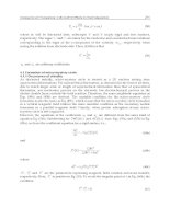
Fig. 1. Force distribution on the manipulator
If the matrix S is not square then S
−1
is pseudo-inverse S
+
. The elements of the S-Matrix
s
i
(q
ai
, q
pi
, q
ei
) comprise the vector that relates f
Bi
, the force of the i
th
chain, and f
XYZi
, the
Cartesian force, which is a result of this force. It can be described in the following formula:

BiiXYZi
fsf
=

. (28)
In the matrix form with the matrix U takes this relation the form:

BB
a
n
1
BXYZ
Uff
s
s
f =
⎥
⎥
⎥
⎦
⎤
⎢
⎢
⎢
⎣
⎡
=
…

…
0
0
. (29)
Now we introduce the Jacobian matrix J

t
of the tree structure:

⎥
⎥
⎥
⎦
⎤
⎢
⎢
⎢
⎣
⎡
=
a
n
1
t
J
J
J
…

…
0
0
, (30)
where J
i
(q

ai
, q
pi
, q
ei
) are the n
a
- Jacobian matrices of the serial kinematic chains. In order to
eliminate the dependencies of the coordinates of the passive joint q
p
for the calculation of
the G Jacobian matrix of parallel manipulator, the matrix J
t
will be parameterised with the
matrix W. After this parameterisation the new matrix no longer represents the mapping
between the joint and Cartesian velocity and force space of the parallel manipulator. In
order to obtain this mapping, the matrices S and U have to be introduced. The matrix S
−1

represents the transformation between the forces from the Cartesian space into the branch
forces. The matrix U constitutes the relation between the forces in the branches and these
Cartesian components. With regards to this transformations, the Jacobian matrix of the
parallel manipulator can be derived from the following relation:

1T
t
TT
USJWG
−+
=

. (31)
This pseudo-inverse Jacobian matrix G
+T
represents the mapping between the Cartesian
force f
XYZ
on the end-effector of parallel manipulator and the forces/torques
()
1
ae
n
R
×
∈
ae
τ in
the manipulator’s structure in the joint space:

XYZ
T
ae
fGτ
+
= . (32)
Automation and Robotics

270
The presented method has the great advantage that the derivation of the serial Jacobian
matrices is much easier than the derivation of the compact Jacobian matrix.
5. A new method for the calculation of the direct dynamics of elastic parallel

manipulators
In this section, the formation of a system as a tree structure for the simultaneous calculation
of the direct dynamics of the elastic parallel manipulator – SCDD is suggested. It is the same
idea as the one used for the inverse dynamics of the Lagrange-D’Alembert formulation.
However, in this system the closed kinematic loop constraints of the elastic parallel structure
are represented by forces and torques, just like in the case of the Lagrangian equations of the
first type. These forces and torques are distributed in the tree structure such that they cause
motion and internal forces which match the motion and mechanical stress in the structure of
the original parallel manipulator.
5.1 Simultaneous Calculation of the Direct Dynamics (SCDD)
The equations of the tree structure have the known form shown in (19). These equations will
now be factored into the equations of motion of the individual serial kinematic chains:

(
)
(
)
(
)
tititititiXYZi
T
ti
tititititititititi
τqDqKfJ
qηqqqCqqM
=+++
++


,

, (33)
for i=1 … n
a
, where i designates one kinematic chain with the associated variables q
ti
= [q
ai

q
pi
q
ei
] and torques τ
ti
= [τ
ai
τ
pi
τ
ei
] of the active τ
ai
and passive τ
pi
joints and additionally
structure torques
τ
ei
. f
XYZi

represents an external force acting on the end of the i
th
-branches of
the tree structure. The equations of the direct dynamics of each such chain can then be
formulated:

(
)
(
(
)
()
)
XYZi
T
tititititititi
titititititititi
fJqDqKqη
qqqCτqMq
−−−−
−=
−


,
1
, (34)
for i=1 … n
a
. Thus, the direct dynamics of each serial kinematic chain can be calculated. The

input for each of these equations are the external forces acting on the end of the particular
serial kinematic chain f
XYZi
and the input torques τ
ai
and τ
pi
. The torques of the elastic DOF
τ
ei
result from the material properties like stiffness and damping. Additionally, they can be
also produced by attached adaptronic actuators. They are independent. The input of the
tree-structure (19) and of the compact parallel manipulator (20) is the torque vector
τ
c
. The
virtual work of both systems is equal (10). The torques of the tree-structure are
interdependent and result from the input torque vector. They represent the constraint
torques/forces of the structure and the drive torques that induce the movement of the
manipulator. The relation between these torques and the input torque vector is established
in (17). However, before these torques can be calculated, one must first calculate the position
(7), velocity (12) and after the differentiation of velocity, the acceleration of the redundant
passive joints as a function of the active joints and the elastic DOF (Beyer, 1928, Stachera,
2005). This is done with the use of the closed kinematic loop constraints (8). Then from the
Derivation and Calculation of the Dynamics of Elastic Parallel Manipulators

271
equations of the reduced system (33) the partial matrices and vectors are taken, which are
associated with the virtual torques of the passive joints:

(
)
(
)
()
tipjXYZi
T
pjtipj
tititipjtitipjpj
qDfJqη
qqqCqqMτ


+++
+= ,
, (35)
for j=1 … n
p
, i=1…n
a
, where the j
th
passive joint belongs to the i
th
kinematic chains. Finally,
the torques
τ
a
that arise from the computed virtual torques τ
p

= [τ
1
… τ
np
] and from the drive
torques
τ
c
of the original parallel structure can be calculated. For that, the Jacobian matrix
(12) is used, which was already derived for the inverse dynamics (17) and (18). This matrix
exists already in a symbolic form, which reduces the amount of work:

p
T
a
p
ca
τ
q
q
ττ
T
⎟
⎟
⎠
⎞
⎜
⎜
⎝
⎛

∂
∂
−=
. (36)
Only the virtual torques (35) of the passive joints from all of the torques and forces in the
robot’s structure are used for the calculation of the torques
τ
a
of active joints. The influence
of the torques and forces
τ
e
of the elastic DOF on the manipulator’s movement is reflected in
the coordinates of the elastic DOF and they were already used for the calculation of the
virtual torques
τ
p
. These torques of the passive τ
p
and active τ
a
joints cause movement in the
tree structure, that correspond to the movement of the original parallel manipulator,
according to the D’Alembert principle of virtual work. In the compact equations of direct
dynamics, the compact torques affect the active joints (20). These torques are accounted for
by the torque and force distributions in the closed-link mechanism. For this reason, the
compact torques should be applied to the active joints of the reduced tree structure in order
to ensure the same operation conditions. Namely:

.0

=
=
p
c,a
τ
ττ
(37)
In order to fulfill this condition, the new forces of the closed-loop constraints acting on the
end of each i
th
–branch, must be calculated, and together with the drive torques supplied to
the partial equations of direct dynamics (34). The difference between the acting torques of
the compact manipulator and the acting torques of the tree structure amounts to:

p
T
a
p
aca
τ
q
q
τττ
T
⎟
⎟
⎠
⎞
⎜
⎜

⎝
⎛
∂
∂
=−=Δ
. (38)
The new constraints forces can be calculated:

[
]
piai
T
tiXYZi
τΔτJf −=
−
ˆ
, (39)
for i=1 … n
a
. Distribution of this force on the manipulator’s structure imply the condition
(37). Now the external forces acting on the end-effector of the manipulator have to be
distributed between all the separate serial kinematic chains. The relation of static (27) and
(29) will be used:

XYZ
1
BXYZ
fUSf
−
= , (40)

Automation and Robotics

272
where f
BXYZ
=[f
XYZ1
… f
XYZi
… f
XYZna
]
T
. These forces (40) and the forces resulting from the
constraints (39) form the common force acting on each serial kinematic chain. The final
formulation for the forces takes the form:

XYZiXYZiXYZi
fff
ˆ
+= , (41)
for i=1 … n
a
. The movement of the tree structure and the movement of the original parallel
manipulator as well as the force and torques distribution in the structure are equal.
This algorithm can be summarized in the followings steps:
1.
Transformation of the system in a reduced system and calculation of the direct dynamics
for each serial kinematic chain separately – simultaneous (34). In order to compute
these equations (in a calculation loop), the torques and forces resulting from the

constraints and from the actuation have to be calculated first.
2.
Calculation of the trajectory of the passive joints based on the non-redundant DOF
(coordinates of the actuated joints and elastic DOF) and the constraints of the closed
kinematic loops of the parallel structure.
3.
Calculation of the virtual torques of the passive joints using the partial equations of the
inverse dynamics of serial kinematic chains (35) and the difference between the torques
of the actuated joints of the reduced system and the original manipulator (38).
4.
Calculation of the forces of constraints for each serial kinematic chain from the virtual
torques of the passive joints and the torque differences (39).
5.
Fusion of the forces of constraints with the external forces acting on the end of each
kinematic chain (41). Setting of the torques and forces of the reduced system (34) to
those of the original parallel manipulator (37).
5.2 Features of the new method
In the Method - Simultaneous Calculation of the Direct Dynamics, SCDD – the system is
segmented into a tree structure, as in the case of the inverse dynamics of Lagrange-
D’Alembert formulation. This is done in order to accelerate the inversion of the inertia
matrix. The most frequently used method, the LU-Gaussian elimination, has the complexity
0(n
3
). For the symmetrical manipulator’s structure with only the rotational joints the
complexity can be written as O((n
a
+n
a
n
ek

)
3
), where n
ek
means the number of the elastic DOF
in particular kinematic chain. In comparison, the complexity for the new distributed
calculation performed for the same type of robots amounts to O(n
a
(1+n
pk
+n
ek
)
3
), where n
pk

represents the number of the passive joints in one kinematic chain. For complex systems the
relation n
pk
«n
ek
is valid. The avoidance of the multiplication between n
a
and n
ek
under the
power of three reduces the computational effort. Therefore, the computation speed of the
direct dynamics in joint space of large scale systems can be significantly accelerated by using
several small matrices instead of one complex matrix. Additionally, the computations of the

direct dynamics with this decomposition can be performed in parallel. In the Table 1 the
complexity of the matrix inversion, number of the necessary arithmetical operations, for
three different robots from the
Collaborative Research Center 562 is shown (Hesselbach et al.,
2005). These calculations were done, with the assumption that in each kinematic chain one
elastic DOF n
ek
exists.
These results show considerable reduction of the calculation complexity by using the
proposed algorithm, even with only one additional elastic DOF in each kinematic chain.
Therefore each kinematic chain can be modelled with more parameters, what is a common
procedure for elastic manipulators.
Derivation and Calculation of the Dynamics of Elastic Parallel Manipulators

273
n
a
n
pk
n
ek
SCDD L-D’A Reduction
FIVE-BAR 2 1 1 54 64 16 %
HEXA 6 2 1 384 1728 78 %
TRIGLIDE 3 2 1 162 729 78 %
Table 1. Complexity of the matrix inversion
Also the calculation of the direct dynamics of rigid body parallel manipulators can benefit
from this new method. The reduced form of the dynamics’ equations can decrease the
number of arithmetic operations needed for the calculation of the model. This problem was
investigated on the base of rigid parallel manipulator F

IVE-BAR (Stachera, 2006b). The model
derived with this new method was compared with a model gained with the standard
Lagrange-D’Alembert Formulation. Since it is a comparison study the exact form of the
manipulator’s model is here not important. The symbolic equations were derived and
simplified with the use of Mathematica
®. All the operations and transformations that are
necessary for the computations of the direct dynamics have been considered.

Number of the operations
Operation Type
SCDD L-D’A
Reduction
+ 192 670 71 %
- 80 302 74 %
* 432 2482 83 %
/ 38 36 -6 %
Table 2. Complexity of the arithmetic operations
The results presented in the Table 2 show a considerable reduction of the computational
effort for each kind of operation excepting division (increasing about 6 %). A digital
processor needs many machine steps for the multiplication, therefore the reduction of this
operation’s number is essential for the general reduction of the computational power for a
model computation. In this case a reduction of 84 % was achieved. This confirms the
applicability of this procedure for the effective reduction of computing power even for a
rigid parallel manipulators.
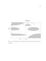
5.3 Verification
The new SCDD method was compared with the L-D’A method in simulation. A model of
elastic planar parallel manipulators F
IVE-BAR was created. A lumped elasticity c
L
= c

R
=
5.464·10
6
N/m was considered in the upper arms of the manipulator, shown in Fig. 2. M
L
and
M
R
represent the motors. The other parameters of this model are not relevant, since it is a
comparison study. A straight line trajectory between two points p
A
and p
E
was chosen. The
models were then controlled by torques, which were created by a rigid body model without
control. The black line represents the reference trajectory. The dark gray line is a result of the
L-D’A model and the light gray line from the SCDD model. It can be seen, that the models
both follow the trajectory with comparable accuracy.
For better comparison of these models, the same trajectories are expressed now with the
help of the forces induced in the branches, F
L
in the left branch and F
R
in the right one, of the
parallel manipulator, shown in Fig.3. A small difference between these forces can be noted.
At the beginning of the simulation the differences are equal to zero, but with the time they
Automation and Robotics

274

change. Apart from the difference between these forces, a good agreement in the vibrations’
behaviour of both systems, frequency, amplitude and phase, can be observed, which
confirms the new proposed method.


Fig. 2. Trajectory and workspace of elastic planar parallel manipulator F
IVE-BAR


Fig. 3. Force in the active rods of the parallel manipulator - comparison


Fig. 4. Distance between two kinematic chains of
FIVEBAR – numerical error of SCDD
The existing differences between the paths traveled by these two elastic models and the
induced forces can be accounted for by the numerical precision. Fig. 4 shows the distance
Derivation and Calculation of the Dynamics of Elastic Parallel Manipulators

275
between the end points of both kinematic chains. This numerical precision causes the
increase in time of the distance between two kinematic chains, that should have been equal
to zero. The dark gray line
Δs = 1·10
−14
m shows the L-D’A and the light gray the SCDD
model. The error is dependent on the sample interval of the simulation: the smaller the
interval, the smaller the error. In the field of numerical methods algorithms are known that
deal with the stabilization of the numerical calculation and increasing of the computation
accuracy (Baumgarte, 1972), which will be the next step in the investigation of this new
algorithm. Despite this numerical error, the analytical approach is confirmed by these

presented results.
6. Conclusion
In this chapter, the Lagrange equation of the first type and Lagrange-D’Alembert
Formulation were introduced around the consideration of elastic modes. To complete the
standard method of Lagrange-D’Alembert, an algorithm for the derivation of the Jacobian
matrix of the parallel manipulator based on the Jacobian matrices of the individual serial
kinematic chains was presented. Originating from this knowledge, a new method was
presented for the simultaneous calculation of the direct dynamics of the parallel and
furthermore the elastic parallel manipulators. The new method shows a significant
reduction of the complexity of the calculation, even for the rigid body manipulators. For the
sophisticated systems this feature is a great advantage. The disadvantage of the presented
method is the numerical stability over long periods of time, which will therefore be the topic
of future researches.
7. References
Baumgarte, J. (1972). Stabilization of constraints and integrals of motion in dynamical
systems.
Computer Methods in Applied Mechanics, Vol.1, pp. 1–36
Beres, W. & Sasiadek, J. Z. (1995). Finite element dynamic model of multilink flexible
manipulators.
Applied Mathematics and Computer Science, Vol. 5, No. 2, pp. 231 – 262,
Technical University Press Zielona Gora, Poland
Beyer, R. (1928). Dynamik der mehrkurbelgetriebe. In:
Zeitschrift fuer angewandte Mathematik
und Mechanik
, Vol. 8, No. 2, pp. 122 – 133
Featherstone, R. & Orin, D. (2000). Robot dynamics: equations and algorithms.
Proceedings of
the IEEE International Conference on Robotics and Automation, pp. 826 – 834, San
Francisco, USA
Hesselbach, J.; Bier, C.; Budde, C.; Last, P.; Maass, J. & Bruhn, M. (2005). Parallel robot

specific control functionalities. In:
Robotic Systems for Handling and Assembly, 2nd
International Colloquium of the Collaborative Research Center 562, Last, P., Budde, C.,
and Wahl, F. M., (Ed.), pp. 93 – 108. Fortschritte in der Robotik Band 9, Shaker
Verlag, Braunschweig, Germany
Kang, B. & Mills, J. K. (2002). Dynamic modeling of structurally-flexible planar parallel
manipulator.
Robotica, Vol. 20, pp. 329–339
Khalil, W. & Gautier, M. (2000). Modelling of mechanical system with lumped elasticity.
Proceedings of the IEEE International Conference on Robotics and Automation,pp. 3965 –
3970, San Francisco, USA
Kock, S. (2001). Parallelroboter mit Antriebredundanz.
PhD thesis, Fortschritt - Berichte VDI,
Duesseldorf - Braunschweig, Germany
Merlet, J P. (2000). Parellel Robots.
Kluwer Academics Publishers, Netherlands.
Automation and Robotics

276
Miller, K. & Clavel, R. (1992). The lagrange-based model of delta-4 robot dynamics.
Robotersysteme, Springer Verlag, Vol. 8, pp. 49–54., Germany
Murray, R. M.; Li, Z. & Sastry, S. S. (1994). A mathematical introduction to robotic
manipulation.
CRC Press LLC, USA
Nakamura, Y. (1991). Advanced robotics: redundancy and optimization.
Addison-Wesley
Publishing Company
, USA
Nakamura, Y. & Ghodoussi, M. (1989). Dynamics computation of closed-link robot
mechanisms with nonredundant and redundant actuators.

IEEE Transactions on
Robotics and Automation, Vol. 5, No. 3, pp. 294–302
Park, F. C.; Choi, J. & Ploen, S. R. (1999). Symbolic formulation of closed chain dynamics in
independent coordinates.
Pergamon: Mechanism and Machine Theory, Vol. 34, pp. 731
– 751
Piedboeuf, J C. (2001). Six methods to model a flexible beam rotating in the vertical plane.
Proceedings of the IEEE International Conference on Robotics and Automation, pp. 2832 -
2839,Seul, Korea
Robinett, R. D.; Dohrmann, C.; Eisler, G. R.; Feddema, J.; Parker, G. G.; Wilson, D. G. &
Stokes, D. (2002). Flexible robot dynamics and controls.
Kluwer Academic/Plenum
Publishers: International Federation for System Research - IFSR, New York, USA
Spong, M. W. & Vidyasagar, M. (1989). Robot dynamics and control.
John Wiley and Sons,
Inc., USA
Stachera, K. (2005). An approach to direct kinematics of a planar parallel elastic manipulator
and analysis for the proper definition of its workspace.
Proceedings of the 11
th
IEEE
Conference on MMAR, Miedzyzdroje, Poland
Stachera, K. (2006a). A new method for the direct dynamics’ calculation of parallel
manipulators.
Proceedings of the 6
th
IEEE World Congress on Intelligent Control and
Automation, Dalian, China
Stachera, K. (2006b). An approach for the simultaneous calculation of the direct dynamics of
parallel manipulators.

Proceedings of the 12
th
IEEE Conference on MMAR,
Miedzyzdroje, Poland
Stachera, K. & Schumacher, W. (2007). Simultaneous calculation of the direct dynamics of
the elastic parallel manipulators.
Proceedings of the 13
th
IEEE IFAC International
Conference on Methods and Models in Automation and Robotics (MMAR), Szczecin,
Poland
Tsai, L W. (1999). Robot analysis: the mechanics of serial and parallel manipulators.
John
Wiley and Sons, Inc., USA
Wang, J. & Gosselin, C. (2000). Parallel computational algorithms for the simulation of
closed-loop robotic systems.
Proceedings of the International Conference on Parallel
Computing Applications in Electrical Engineering (PARELEC2000), IEEE Computer
Society, pp. 34 – 38, Washington, DC, USA
Wang, J.; Gosselin, C. M. & Cheng, L. (2002). Modeling and simulation of robotic systems
with closed kinematic chains using the virtual spring approach.
Kluwer Academic
Publishers, Springer Netherlands, Multibody System Dynamics, Vol. 7, No. 2, pp. 145
– 170
Wang, X. & Mills, J. K. (2004). A fem model for active vibration control of flexible linkages.
Proceedings of the IEEE International Conference on Robotics and Automation (ICRA),
pp. 4308–4313, New Orleans, USA
Yiu, Y. K.; Cheng, H.; Xiong, Z. H.; Liu, G. F. & Li, Z. X. (2001). On the dynamics of parallel
manipulators.
Proceedings of the IEEE International Conference on Robotics and

Automation (ICRA), pp. 3766 – 3771, Seul, Korea
16
Orthonormal Basis and Radial Basis Functions
in Modeling and Identification of Nonlinear
Block-Oriented Systems
Rafał Stanisławski and Krzysztof J. Latawiec
Department of Electrical, Control and Computer Engineering
Opole University of Technology
Poland
1. Introduction
Nonlinear block-oriented systems, including the Hammerstein, Wiener and feedback-
nonlinear systems have attracted considerable research interest both from the industrial and
academic environments (Bai, 1998), (Greblicki, 1989), (Latawiec, 2004), (Latawiec et al.,
2003), (Latawiec et al., 2004), (Pearson & Pottman, 2000).
It is well known that orthonormal basis functions (OBF) (Bokor et al., 1999) have proved to
be useful in identification and control of dynamical systems, including nonlinear block-
oriented systems (Gómez & Baeyens, 2004), (Latawiec, 2004), (Latawiec et al., 2003),
(Latawiec et al., 2006), (Latawiec et al., 2004), (Stanisławski et al., 2006). In particular, an
inverse OBF (IOBF) modeling approach has been effective in identification of a linear
dynamic part of the feedback-nonlinear and Hammerstein systems (Latawiec, 2004),
(Latawiec et al., 2004). On the other hand, regular OBF (ROBF) modeling approach has
proved to be useful in identification of the Wiener system. The approaches provide the
separability in estimation of linear and nonlinear submodels (Latawiec et al., 2004), thus
eliminating the bilinearity issue detrimentally affecting e.g. the ARX-based modeling
schemes (Latawiec, 2004), (Latawiec et al., 2003), (Latawiec et al., 2006), (Latawiec et al.,
2004). The IOBF modeling approach is continued to be efficiently used here to model a
linear dynamic part of the feedback-nonlinear and Hammerstein systems and regular OBF
modeling approach is used to model a linear part of the Wiener system.
The problem of modeling of a nonlinear static part of the nonlinear block-oriented system
can be classically tackled using e.g. the polynomial expansion (Latawiec, 2004), (Latawiec et

al., 2004) or (cubic) spline functions. Recently, a radial basis function network (RBFN) has
been used to model a nonlinear static part of the Hammerstein and feedback-nonlinear
systems and a very good identification performance has been obtained (Hachino et al.,
2004), (Stanisławski, 2007), (Stanisławski et al., 2007). The concept is extended here to cover
the Wiener system.
This paper presents a new strategy for nonlinear block-oriented system identification, which
is a combination of OBF modeling for a linear dynamic part and RBFN modeling for a
nonlinear static element. The effective OBF approach is finally coupled with the RBFN
modeling concept, giving rise to the introduction of a powerful method for identification of
the nonlinear block-oriented system.
Automation and Robotics

278
2. Regular and inverse OBF modelling concept
2.1 Regular OBF modeling
It is well known that an open-loop stable linear discrete-time system described by the
transfer function G(q) can be represented with an arbitrary accuracy by the model
∑
=
=
M
i
ii
qLcqG
1
)()(
ˆ
, including a series of orthonormal transfer functions L
i
(q) and the

weighting parameters c
i
, i=1, ,M, characterizing the model dynamics. Thus, the model of
the system can be written as (Latawiec, 2004), (Latawiec et al., 2006), (Latawiec et al., 2004)

∑
=
=
M
i
ii
tuqLcty
1
)()()(
ˆ
(1)
Various OBF can be used in (1). Two commonly used sets of OBF are simple Laguerre and
Kautz functions. These functions are characterized by the ‘dominant’ dynamics of a system,
which is given by a single real pole (p) or a pair of complex ones (p, p*), respectively.
In case of discrete Laguerre models to be exploited hereinafter, the orthonormal functions

1
2
1
1
),(
−
⎥
⎦
⎤

⎢
⎣
⎡
−
−
−
−
=
i
i
pq
pq
pq
p
pqL i=1, ,M (2)
consist of a first-order low-pass factor and (i-1)th-order all-pass filters. Dominant Laguerre
pole p can be selected in an experimental way or can be determined with the aid of the
stochastic gradient (SG) estimator (Boukis et al., 2006), (Oliveira, 2000).
2.1 Inverse OBF modeling
In case of use of the inverse OBF (IOBF) concept to model a linear dynamic part, the model
equation can be presented in form

)()(
ˆ
)(
ˆ
1
tutyqG =
−
(3a)

)()(
ˆ
)( tutyqR = (3b)
where FIR model R(q)=
1
1
1
1
1
10

++−
−
−
+
−
+++++
dL
Ldd
dd
qrqrrqrqr
is the inverse of the system
model
)(
ˆ
qG
. In the IOBF concept, the inverse R(q) of the system is modeled using OBF. An
OBF modeling approach can now be applied to equation (3b) instead of (3a) and finally we
can present equation (1) in the following form (Latawiec et al., 2003)

()
()
)()(),(
10
1
tedtutypqLcy
i
M
i
i
t +−=+
∑
=
β
(4)
where e
1
(t) is the equation error, d is the time delay of the system,
β
0
and c
i
i=1,…,M are the
OBF model parameters.
3. RBF network
The nonlinear function approximated by a Radial Basis Functions Network (RBFN) consists
of two layers of neurons (one hidden and one output layer). The hidden layer consists of m
Orthonormal Basis and Radial Basis Functions in Modeling and Identification
of Nonlinear Block-Oriented Systems

279
neurons, where each neuron implements the radial activated function. The output layer
consists of one linear neuron which realizes weighted sum of outputs of hidden layer
neurons. The output of RBFN is described by the equation
))((
1
)( tu
i
i
wtx
i
m
φ
∑
=
= (5)
where w
i
, i=1,…,m are the weighting coefficients and
φ
i
(u(t)) are the outputs of hidden layer
neurons. Typically, the Gaussian function is used as an activation function in RBFN. The
Gaussian functions are modeled by two parameters characterizing their centers
α
i
and wides
σ
i

. In this case the
φ
i
(u(t)) is given by the equation

(
)
2
2
/)(exp))((
iii
kutu
σαφ
−−=
for i=1, ,m (6)
where ||.|| is the Euclidian norm.
Important advantage of the RBF network is that the weighting coefficients w
i
, i=1,…,m can
by estimated by using classical, linear estimation schemes e.g. recursive/adaptive least
squares (RLS/ALS), or least mean squares (LMS). The centers
α
i
and wides
σ
i
(i=1,…,m) of
the RBF can be determined with the aid of the stochastic gradient (SG) estimator (Kim et al.,
2006), genetic algorithm (Hachino et al., 2004) or other optimization methods. However, in
practical applications, the optimization of the

α
i
and
σ
i
is not absolutely necessary. It has
been found in simulations (Stanisławski, 2007) that RBFN without optimization (with
regular distribution of the centers and constant widths) can produce satisfactory solutions.
3. Nonlinear block-oriented systems
3.1 Hammerstein system
The Hammerstein system consists of two cascaded elements, where the first one is a
nonlinear memoryless gain and the second one is a linear dynamic model. The whole
Hammerstein system can be described by the equation

[
]
[
]
)()()()())(()()( tetxqGtetufqGty
HH
+=+=
(7)
where G(q) models a dynamic linear part, f(.) describes a nonlinear function, x(t) is the
unmeasured output of the nonlinear part and e
H
(t) is the error/disturbance term. An
alternative output error/disturbance formulation is also possible.
Combining equations (4),(5) and (7) we arrive at the equation describing the whole
Hammerstein system

()
()
)())((
1
),(
10
1
tedtu
i
i
wtypqLcy
i
m
i
M
i
i
t +−
=
=+
∑∑
=
φβ
(8)
Assuming that w
j
=
β
0
w

j
, i=1…m, the model output from the Hammerstein system can be
finally given as

∑∑
==
−+−=
m
j
j
j
M
i
ii
dtwtypqLc
11
)()(),((
ˆ
φ
)ty
(9)
which can be presented in the linear regression form
Automation and Robotics

280

θϕ
)()(
ˆ
tty

T
= (10)
where
)(t
T
ϕ
=[-v
1
(t) -v
M
(t)
φ
1
(t-d)
φ
2
(t-d)
φ
m
(t-d)],
θ
=[c
1
c
M
w
1
w
2
w

m
] and
v
i
(t)=L
i
(q,p)y(t). Unknown parameters
θ
of the model can be estimated by the familiar
recursive least squares (RLS) or least mean squares (LMS) algorithms.
3.2 Wiener system
In a single-input single-output Wiener system, a linear dynamic part is cascaded with a
nonlinear static element. The output )(
ˆ
ty of the Wiener model, or the system output
predictor, can be calculated as

(q)u(t)] G[f (t)y
ˆ
ˆ
ˆ
=
(11)
Since a nonlinear static characteristic is invertible we can rewrite equation (11) in form

)()( tuqGtyf
ˆ
)](
ˆ
[

ˆ
1
=
−
(12)
The function
)](
ˆ
[
ˆ
1
tyf
−
can be approximated with RBF network. Finally, we arrive at the
linear regression function
))(()()((
ˆ
11
1
ty
i
wtuqLc
i
m
i
M
i
ii
φ
∑∑

==
−
−=)ty
(13)
where
ii
i
ww
α
−=
(i=1, ,m), which can be presented in the familiar form
θϕ
)()(
ˆ
tty
T
=
,
with
)(t
T
ϕ
= [ v
1
(t) -v
M
(t) -
φ
1
(y(t)) -

φ
2
(y(t)) -
φ
m
(y(t))],
θ
=[c
1
c
M
w
1
w
2
w
m
] and
v
i
(t)=L
i
(q,p)u(t), i=1, ,M.
3.3 Feedback-nonlinear system
In the block-oriented feedback-nonlinear system, the output of the linear dynamic part is fed
(negatively) back to the input through the static nonlinearity, so that the whole system can
be described by the equation

[
]

[]
)()()()(
)())(()()()(
tetxtuqG
tetyftuqGty
F
F
+−=
+
−
=
(14)
where e
F
(t) is the error/disturbance term. Combining equations (4),(5) and (14) we arrive at
the equation describing the whole, IOBF-related feedback-nonlinear system (Stanisławski et
al., 2007)

()
()
)())((
1
)(),(
0
1
tedty
j
j
wdtutypqLcy
j

m
i
M
i
i
t +
⎥
⎥
⎦
⎤
⎢
⎢
⎣
⎡
−
=
−−=+
∑∑
=
φβ
(15)
Putting w
j
=
β
0
w
j
, j=1…m, the output from the feedback-nonlinear system can be finally given
as

Orthonormal Basis and Radial Basis Functions in Modeling and Identification
of Nonlinear Block-Oriented Systems

281

()
()
)())((
1
),()(
1
0
tedty
j
j
wtypqLcdtuy
j
m
i
M
i
i
t +−
=
−−−=
∑∑
=
φβ
(16)
The equation (16) can be presented in the linear regression form, with

)(t
T
ϕ
=[u(t-d) -v
1
(t)
-v
M
(t) -
φ
1
(y(t-d)) -
φ
2
(y(t-d)) -
φ
m
(y(t-d))],
θ
=[
β
0
c
1
c
M
w
1
w
2

w
m
] and v
i
(t)=L
i
(q,p)y(t).
Clearly, owing to the IOBF modeling approach applied, the linear and nonlinear submodels
are separated from each other so that the bilinearity issue is eliminated here.
4. Simlation experiments
In the Matlab/Simulink environment, we comparatively analyze the three presented
nonlinear block-oriented OBF/RBFN-related models consisting of 1) Hammerstein IOBF
related model, 2) Wiener regular OBF related model and 3) feedback-nonlinear IOBF related
model. For example, consider the magnetic levitation process which has been simulated as a
demo in the Matlab/Simulink environment. Our main goal is to analyze efficiency of the
approach in view of their possible use in on-line identification (and control). Performance of
parameter estimation is evaluated by means of the mean square prediction error (MSPE).
MSPE is described by the equation

∑
=
−=
N
t
tytyNMSPE
1
2
))(
ˆ
)(()1(

(17)

The system is excited by a random number generator with regular distribution <0.5, 4>.
Additionally, the system is corrupted with the input and output noises (e
i
(t) and e
o
(t)), which
are supplied from a Gaussian random number generators with N(0,
δ
i
) and N(0, δ
o
),
respectively. For estimation of weights of the RBFs and parameters of the dynamical model
we use a classical RLS algorithm.
Table 1 specifies the results of a comparative analysis of the performance of the three models
for M=6 and m=9.

δ
i
δ
o

Hammerstein
system
Wiener system
Feedback-nonlinear
system
0 0 8.851 e-6 0.2437 1.008 e-5

0.005 0 2.167 e-5 1.123 9.236 e-5
0.01 0 4.337 e-5 1.287 9.582 e-5
0 0.005 2.752 2.231 2.838
0 0.01 5.188 3.226 4.95
0.005 0.005 2.921 3.406 2.792
Table 1. MSPE of the Hammerstein, Wiener and feedback-nonlinear models
Automation and Robotics

282
The results in Table 1 show that the high accuracy of identification has been obtained for the
IOBF/RBFN-based models (Hammerstein and feedback-nonlinear models). The reasons are
1) the specific, structure of the IOBF-related model, 2) numerical conditioning of the
covariance matrix for the IOBF-based estimation problem is essentially better than that for
the OBF-based one. However, the inconvenience of IOBF-related models is the high
sensitivity on the output error due to the equation error structure. Table 1 shows that the
Wiener model cannot provide sufficiently high accuracy of the identification problem,
causing that the RBF network in the Wiener system models the inversion of the nonlinear
function f(.). The calculation of the original function on the basis of RBF network is
ambiguous and badly numerical conditioned. Finally, only the Wiener model gives the
satisfy results for the system corrupted with the high-level disturbances.
Plots of the actual output and its reconstruction by Hammerstein, Wiener and Feedback
nonlinear models presented in Fig. 1 and Fig. 2 confirm very good performance of
identification for Hammerstein and Feedback nonlinear models and poor performance for
Wiener model, respectively.

15 20 25 30 35 40 45 50 55 60 65
1
2
3
4

5
6
t
[
s
]
][
)(
),(
ˆ
cm
ty
ty
15 20 25 30 35 40 45 50 55 60 65
1
2
3
4
5
6
][
)(
),(
ˆ
cm
ty
ty
t
[
s

]

Fig. 1. Plots of actual (solid-black) vs. predicted (dashed-red) outputs of the Hammerstein
system (left) and feedback-nonlinear system (right)

][
)(
),(
ˆ
cm
ty
ty
t
[
s
]
15 20 25 30 35 40 45 50 55 60 65
1
2
3
4
5
6

Fig. 2. Plots of actual (solid-black) vs. predicted (dashed-red) outputs of the Wiener system
Orthonormal Basis and Radial Basis Functions in Modeling and Identification
of Nonlinear Block-Oriented Systems

283
7. Conclusion

The paper has presented the solutions to the nonlinear identification problem for the various
nonlinear block-oriented systems using OBF-related models and RBF network. We have
demonstrated that the Wiener model based on regular OBF modeling concept cannot
provide sufficiently high performance of the identification problem. This is mainly to due
with inversion problem of RBF network.
Results of a simulation analysis have shown that the strategy using the IOBF modeling
concept in Hammerstein and feedback-nonlinear model can provide a very good
performance, both in terms of low prediction errors and accurate reconstruction of the
nonlinear characteristics, in addition to high computational efficiency.
8. References
Bai E.W. (1998). An optimal two-stage identification algorithm for Hammerstein-Wiener
nonlinear systems. Automatica, Vol. 34, pp. 333-338.
Bokor J., Heuberger P., Ninness, B., Oliveira e Silva, T., Van den Hof P. & Wahlberg, B.
(1999). Modelling and identification with orthogonal basis functions. Proc.
Preconference Workshop, 14
th
IFAC World Congress, Beijing, P.R. China.
Boukis C., Mandic D.P., Constantinides A.G. & Polymenakos L.C. (2006). A Novel
Algorithm for the Adaptation of the Pole of Laguerre Filters. IEEE Signal Processing
Letters, Vol. 13, No. 7, pp. 429 - 432.
Greblicki W. (1989). Nonparametric orthogonal series identification of Hammerstein
systems. International Journal of Systems Science, Vol. 20, No. 12, pp. 2355-2367.
Gómez J.C. & Baeyens E. (2004). Identification of block-oriented nonlinear systems using
orthonormal bases. Journal of Process Control, Vol. 14, No. 6, pp. 685-697
Hachino T., Deguchi K. & Takata H. (2004). Identification of Hammerstein model using
radial basis function networks and genetic algorithm. Proc. 5th Asian Control
Conference, Vol. 1, pp. 124-129.
Kim N.Y., Byun H.G. & Kwon K.H. (2006). Learning Behaviors of Stochastic Gradient Radial
Basis Function Network Algorithms for Odor Sensing Systems. ETRI journal, Vol.
28, No. 1.

Latawiec K.J. (2004) The Power of Inverse Systems in Modeling and Control of Linear and
Nonlinear Systems. Vol. 167, Opole University of Technology Press, Opole, Poland.
Latawiec K.J., Marciak C., Hunek W. & Stanisławski R. (2003) A new analytical design
methodology for adaptive control of nonlinear block-oriented systems. Proc. 7th
World Multi-Conference on Systemics, Cybernetics and Informatics, Vol. XI, pp. 215-220,
Orlando, Florida, USA.
Latawiec K.J., Marciak C. & Oliveira G.H.C.: (2006). A new control-oriented modeling
methodology for a series DC motor. Electromagnetic Fields in Mechatronics, Electrical
and Electronic Engineering, Wiak S., Krawczyk A. & Fernandez X.L.M. (Eds.), IOS
Press, Studies in Applied Electromagnetics and Mechanics, Vol. 27, Chapter_B_13.
Latawiec K.J., Marciak C., Rojek R. & Oliveira G.H.C. (2003). Linear parameter estimation
and predictive constrained control of Wiener/Hammerstein systems. Proc. 13th
IFAC Symposium on System Identification, pp. 359-364, Rotterdam, The Netherlands.
Automation and Robotics

284
Latawiec K.J., Marciak C., Stanisławski R. & Oliveira G.H.C. (2004) The mode separability
principle in modeling of linear and nonlinear blockoriented systems. Proc. the 10th
IEEE MMAR Conference (MMAR’04), Vol. 1, pp. 479-484, Miedzyzdroje, Poland.
Oliveira S.T. (2000). Optimal pole conditions for Laguerre and two-parameter Kautz models:
a survey of known results. Proc. 12th IFAC Symp. on System Identification
(SYSID'2000), pp. 457-462, Santa Barbara, CA, USA.
Pearson R.K. & Pottman M. (2000). Gray-box identification of block-oriented nonlinear
models. Journal of Process Control, Vol. 10, pp. 301-315.
Stanisławski R., Latawiec K.J. & Stanisławski W. (2006). Modeling of a boiler proper using a
complex structure model by means of multivariable orthonormal basis functions.
Proc. 12th IEEE MMAR Conference (MMAR’06), pp. 935-938, Miedzyzdroje, Poland.
Stanisławski R. (2007). Hammerstein system identification by means of orthonormal basis
functions and radial basis functions. Emerging Technologies, Robotics and Control
Systems, Pennacchio S. (Eds.), Internationalsar, Vol. 2, pp. 69-73, Palermo, Italy.

Stanisławski R., Latawiec K.J. & Hunek W.P. (2007). Identification of feedback-nonlinear
systems by means of orthonormal basis and radial basis functions. Proc. 13th IEEE
IFAC IC MMAR 2007, pp. 611-616, August 2007, Szczecin, Poland.
17
Control System of Underwater Vehicle Based on
Artificial Intelligence Methods
Piotr Szymak and Józef Małecki
Polish Naval Academy
Poland
1. Introduction
One of the main development directions of an underwater technology are robots, which are
working under the surface of a water. Using of these unmanned vehicles enables
exploration at bigger depths and in more hazardous conditions (Kubaty & Rowiński, 2001).
Correctness of realization of different underwater works requires precise control of robot’s
movement in underwater environment.


Fig. 1. Remotely operated vehicle called Ukwial
In the case of underwater robot is object of nonlinear dynamics and works in marine
environment with different disturbances robust nonlinear control method may be applied.
An example of this kind application is designed and verified automatic control system of
underwater vehicle called Ukwial (fig. 1).
Problem of underwater vehicle’s control is considered by several scientific centers
(particularly in the United States – Florida Atlantic University, Massachusetts Institute of
Technology, Naval Postgraduate School in Monterey; in Japan – Osaka University, in
Automation and Robotics

286
Norway – University of Trondheim, in Poland – Szczecin University of Technology, Polish
Naval Academy in Gdynia). Direct results of researches are usually inaccessible for the sake

of their commercial or military application. While published results of researches are
concerned mainly on basic problems: control of course and control of draught.
This chapter contribute into domain of underwater vehicle’s control results of numerical
and experimental researches of remotely operated vehicle Ukwial, which is used in Polish
Navy. Using of presented robust nonlinear control method helps operators of Ukwial in
their daily work.
In the chapter selected aspects of steering an underwater vehicle along desired trajectory
have been developed. The fuzzy data processing has been applied for compensation of the
nonlinear underwater vehicle’s dynamics and influence of environmental disturbances. It
has enabled to calculate command signals driving the vehicle with set values of movement’s
parameters. An architecture of the selected fuzzy logic controllers has been presented.
Moreover, the results of computer simulations and experimental research of remotely
operated vehicle Ukwial have been inserted.
2. Mathematical model of an underwater vehicle
Nonlinear model in six degrees of freedom has been accepted to simulate movement of the
underwater vehicle (Fossen, 1994). This movement has been analyzed in two coordinate
systems:
1. the body-fixed coordinate system, which is movable,
2. the earth-fixed coordinate system, which is immovable.
While for the aim of movement description, notation of physical quantities according to
SNAME (The Society of Naval Architects and Marine Engineers) has been accepted. Underwater
vehicle’s movement is described with the aid of the six equations of motion, where the three
first equations represent the translational motion and the three last equation represent the
rotational motion. These six equations can be expressed in a compact form as:
M
ν

+ C(
ν
)

ν
+ D(
ν
)
ν
+ g(
η
) + U(
ν
)
ν
=
τ
(1)
Here
ν
=[u,v,w,p,q,r] is the body-fixed linear and angular velocity vector,
η
=[x,y,z,
φ
,
θ
,
ψ
] is the
earth-fixed coordinates of position and Euler angles vector and
τ
=[X,Y,Z,K,M,N]
T
is the

vector of forces and moments of force influenced on underwater vehicle. M is a inertia
matrix, which is equal a rigid-body inertia matrix and added mass inertia matrix. C is a
Coriolis and centripetal matrix, which is a sum of rigid-body and added mass Coriolis and
centripetal matrixes. D is a hydrodynamic damping matrix and g is a restoring forces and
moments matrix. U is a damping matrix generated by a cable called an umbilical cord.
Underwater vehicle is supplied and can be controlled via the umbilical cord.
After making assumption that underwater vehicle has three planes of symmetry, it moves
with small speed in a viscous liquid and an origin of movable coordinate system covers with
vehicle’s centre of gravity, specific form of matrixes with nonzero values of diagonal’s
elements has been obtained (Fossen, 1994). According to earlier researches (Szymak &
Małecki, 2007) these elements were calculated on the base of geometrical parameters of
remotely operated vehicle (abbr. ROV) Ukwial.
Whereas Coriolis and centripetal matrixes were omitted because of small numerical values,
unimportant in computer simulation.
Control System of Underwater Vehicle Based on Artificial Intelligence Methods

287
Nonlinear mathematical model of an underwater vehicle has been considered in more detail
in (Fossen, 1994).

α
14
=
0
X
Y
X
Z
α
1

4
α
14
α
1
4
α
14
a)
b)
α
14
=
0
X
Y
X
Z
α
1
4
α
14
α
1
4
α
14
a)
b)

Fig. 2. Location of particular Ukwial’s propellers in: a) horizontal and b) vertical plane
ROV Ukwial was designed in Underwater Technology Department from Gdansk University
Of Technology. It is remotely operated and powered from board. A construction of Ukwial
is based on cubicoid-shape frame, where all propulsion system and added equipment are
mounted to the frame. This underwater vehicle has specific propulsion system, consisted of:
four, three blade screw propellers in horizontal plane (fig. 2, here α
14
= 29°) and two, three
blade screw propellers in vertical plane. Each propeller is electrically driven.
Presented propulsion system enables to move underwater vehicle in water with average
speed 0,5-1,0 m/s and allows to control ROV’s movement in five degrees of freedom (three
translations motions: in longitudinal axis of symmetry x
o
, in lateral axis of symmetry y
o
and
in vertical axis of symmetry z
o
, and two rotations around lateral axis of symmetry y
o
and
around z
o
axis).
Moreover specific location of propellers in horizontal plane (at an angle of 29° to the
longitudinal axis of symmetry) gives possibility of steering this ROV in case of one of
propellers is out of order.
3. Architecture of Ukwial’s control system
Designed automatic control system of underwater vehicle consists of (fig. 3):

1. supervisory control unit, which is responsible for setting values of movement’s
parameters, turning on and off individual controllers at the proper moments,
2. the four controllers of: course, displacement in X axis, displacement in Y axis and
draught, which generate adequate control signals: moment of force N, force in X axis,
force in Y axis and force Z.
Proportional-derivative action controllers based on the fuzzy logic have been applied to
carry out control of course, displacement in X axis, displacement in Y axis and draught
(fig. 4), where parameter p is adequate course, coordinate x, y or z.
Using of fuzzy logic method in FPD controllers depends on selection (Driankov et al., 1996):
Automation and Robotics

288
1. number, type and position’s parameters of membership function of the input and
output variables,
2. fuzzy inference rules, which create base of rules.


draught’s
controller

Z
N
-Y
X

controller of
displacement in Y axis
controller of
displacement
in X axis

Supervisory
control unit
course’s
controller

Fig. 3. Automatic control system of underwater vehicle called Ukwial



+
_

error
e

change
of error
Δe

set value of
parameter
p

UNDERWATER
VEHICLE
vector of
state [
ν
,
η

]

amplification
derivative
Fuzzy
Inference System
actual value of parameter
p
a

control
signal
τ

FPD


Fig. 4. Block diagram of fuzzy proportional-derivative controller FPD
Membership functions for linguistic input variables: error signal and derived change in
error and output variable - control signal were tuned with the aid of the mathematical
model simulation of the automatic controlled underwater vehicle. Direct and integral
indexes were used to evaluate control quantity of designed control system. Results of this
selection method for course controller have been presented in fig. 5.
Control System of Underwater Vehicle Based on Artificial Intelligence Methods

289
Presented membership functions selection allow to create base of 35 rules (fig. 6). Particular
rule could be read from the intersection of specified row and column. For the first row and
first column following rule has been obtained:
If error of course is Negative Large and change in error of course is Negative Large

then moment of force N is Negative Large
Rules from the Mac Vicar-Whelan’s standard base were chosen as the control rules (Garus &
Kitowski, 2001).

NL NM NS Z PS PM PL
NL NM Z PM PL
NL NM NS Z PS PM PL
error of course
change in error of course
control signal – moment of force N
degree of membership degree of membership degree of membership

Fig. 5. Fuzzy partition of the universe of discourse of course
Automation and Robotics

290

error of course


N
L
N
M
N
S Z PS PM P L

N
L

N
L

N
L

N
L

N
M Z PS

PL


N
S
N
L
N
L
N
M
N
S PS PM PL

Z
N
L
N

M
N
M Z PM PM PL

PS

N
L

N
M
N
S


PS

PM PL

PL


change in error of
course
PL
N
L
N
S Z PM PL PL PL

control signal - moment of force N

Fig. 6. Base of rules of course controller (NL – Negative Large, NM – Negative Mean, NS –
Negative Small, Z – zero, PS – Positive Small, PM – Positive Mean, PL – Positive Large)
4. Results of numerical researches
Computer simulations were carried out in the Matlab environment on the platform
computer PC / Windows XP. At the beginning each controller was tuned with the aid of
direct and integral control quantity indexes.
Subsequently whole automatic control system of underwater vehicle Ukwial (fig. 3) was
tested. Researches were carried out in simulated underwater environment with or without
an influence of sea current with defined parameters: V
p
(velocity) and
α
p
(an angle between
magnetic north and direction of affecting in horizontal plane).
Tested task of designed control system was to steer the underwater vehicle along desired
trajectory in vertical plane XZ (fig. 7).


X
Z
2 m
5 m
ψ
zad
= 90

0

Fig. 7. Desired trajectory of Ukwial in vertical plane
Presented course of desired trajectory (fig. 7) comes from nature of the mission executed by
the underwater vehicle, which is inspection of hull’s part located below surface of water
(fig. 8).
Control System of Underwater Vehicle Based on Artificial Intelligence Methods

291


X


Y



d
s
g
= 2 m



desired

angle of view 52
0
d

k

= 2 m
underwater vehicle

(top view)

desired
trajectory

camera

desired
course 90
0
hull of warship



(top view)



angle of view
of camera
α

k
= 70
0

Fig. 8. Desired trajectory of Ukwial in vertical plane (top view)
From the fig. 8 results additional condition that a course of Ukwial should be controlled to
the value of desired course 90°, what guarantees monitoring of whole underwater part of
inspected hull.
Assuming that camera of an underwater vehicle is immovable and underwater vehicle
moves along specified trajectory (fig. 7, fig. 8) following maximal errors of controlled
parameters were calculated: maximal error in X axis
Δ
x = ± 0,4 m, maximal error in Y axis
Δ
y = ± 0,5 m, maximal error of course
Δψ
=± 9
°
.
To illustrate changes of 4 parameters (3 coordinates and an angle of course) on single figure
following method has been accepted (fig. 9): changes of a course at the discrete points of
trajectory are presented as line segments covering with longitudinal axis of symmetry.
Additionally direction of affecting sea current was visualized in form of a red arrow, what
helps to illustrate conditions of moving in an underwater environment.

Trajectory of underwater vehicle in space XYZ Changes of course during motion along trajectory
coordinate y [m] coordinate y [m]
coordinate x [m]
coordinate x [m]
coordinate z [m]
coordinate z [m]
a)

Automation and Robotics

292
Trajectory of underwater vehicle in space XYZ Changes of course during motion along trajectory
coordinate y [m] coordinate y [m]
coordinate x [m]
coordinate x [m]
coordinate z [m]
coordinate z [m]
b)

Trajectory of underwater vehicle in space XYZ Changes of course during motion along trajectory
coordinate y [m] coordinate y [m]
coordinate x [m]
coordinate x [m]
coordinate z [m]
coordinate z [m]
c)

Trajectory of underwater vehicle in space XYZ Changes of course during motion along trajectory
coordinate y [m] coordinate y [m]
coordinate x [m]
coordinate x [m]
coordinate z [m]
coordinate z [m]
d)

Fig. 9. Automatic steering of underwater vehicle along desired trajectory a) without sea
current and with different sea currents: b) V
p

= 0,5 m/s,
α
p
= 0
0
, c) V
p
= 0,9 m/s,
α
p
= 0
0

and d) V
p
= 0,5 m/s,
α
p
= 45
0