Engineering Materials Vol II (microstructures_ processing_ design) 2nd ed. - M. Ashby_ D. Jones (1999) WW Part 3 ppsx
Bạn đang xem bản rút gọn của tài liệu. Xem và tải ngay bản đầy đủ của tài liệu tại đây (633.33 KB, 27 trang )
Case studies in phase diagrams 45
4.3 A single-pass zone refining operation is to be carried out on a long uniform bar of
aluminium containing an even concentration C
0
of copper as a dissolved impurity.
The left-hand end of the bar is first melted to produce a short liquid zone of length
l and concentration C
L
. The zone is then moved along the bar so that fresh solid
deposits at the left of the zone and existing solid at the right of the zone melts. The
length of the zone remains unchanged. Show that the concentration C
S
of the fresh
solid is related to the concentration C
L
of the liquid from which it forms by the
relation
C
S
= 0.15C
L
.
At the end of the zone-refining operation the zone reaches the right-hand end of
the bar. The liquid at the left of the zone then begins to solidify so that in time the
length of the zone decreases to zero. Derive expressions for the variations of both
C
S
and C
L
with distance x in this final stage. Explain whether or not these expres-
sions are likely to remain valid as the zone length tends to zero.
The aluminium-copper phase diagram is shown below.
700
800
600
500
400
300
200
01020
30
40
50
60
70
Weight% Cu
548˚C
α
α
L
660˚C
(CuAl
2
)
Al
Temperature (˚C)
+
α
θ
+
θ
L
Answers:
C
Cl
lx
CC
l
lx
LS
.
;
.
=
−
=
−
0
085
0
085
015
46 Engineering Materials 2
Chapter 5
The driving force for structural change
Introduction
When the structure of a metal changes, it is because there is a driving force for the
change. When iron goes from b.c.c. to f.c.c. as it is heated, or when a boron dopant
diffuses into a silicon semiconductor, or when a powdered superalloy sinters together,
it is because each process is pushed along by a driving force.
Now, the mere fact of having a driving force does not guarantee that a change will
occur. There must also be a route that the process can follow. For example, even
though boron will want to mix in with silicon it can only do this if the route for the
process – atomic diffusion – is fast enough. At high temperature, with plenty of thermal
energy for diffusion, the doping process will be fast; but at low temperature it will be
immeasurably slow. The rate at which a structural change actually takes place is then
a function of both the driving force and the speed, or kinetics of the route; and both must
have finite values if we are to get a change.
We will be looking at kinetics in Chapter 6. But before we can do this we need to
know what we mean by driving forces and how we calculate them. In this chapter we
show that driving forces can be expressed in terms of simple thermodynamic quantit-
ies, and we illustrate this by calculating driving forces for some typical processes like
solidification, changes in crystal structure, and precipitate coarsening.
Driving forces
A familiar example of a change is what takes place when an automobile is allowed to
move off down a hill (Fig. 5.1). As the car moves downhill it can be made to do work
– perhaps by raising a weight (Fig. 5.1), or driving a machine. This work is called the
free work, W
f
. It is the free work that drives the change of the car going downhill and
provides what we term the “driving force” for the change. (The traditional term driv-
ing force is rather unfortunate because we don’t mean “force”, with units of N, but
work, with units of J).
How can we calculate the free work? The simplest case is when the free work is
produced by the decrease of potential energy, with
W
f
= mgh. (5.1)
This equation does, of course, assume that all the potential energy is converted into
useful work. This is impossible in practice because some work will be done against
friction – in wheel bearings, tyres and air resistance – and the free work must really be
written as
The driving force for structural change 47
Fig. 5.1. (a) An automobile moving downhill can do work. It is this
free work
that drives the process. (b) In
the simplest situation the free work can be calculated from the change in potential energy,
mgh
, that takes
place during the process.
W
f
≤ mgh. (5.2)
What do we do when there are other ways of doing free work? As an example, if
our car were initially moving downhill with velocity v but ended up stationary at the
bottom of the hill, we would have
W
f
≤ mgh +
1
2
mv
2
(5.3)
instead. And we could get even more free work by putting a giant magnet at the
bottom of the hill! In order to cover all these possibilities we usually write
W
f
≤ −∆N, (5.4)
where ∆N is the change in the external energy. The minus sign comes in because a
decrease in external energy (e.g. a decrease in potential energy) gives us a positive
output of work W. External energy simply means all sources of work that are due
solely to directed (i.e. non-random) movements (as in mgh,
1
2
mv
2
and so on).
A quite different source of work is the internal energy. This is characteristic of the
intrinsic nature of the materials themselves, whether they are moving non-randomly
or not. Examples in our present illustration are the chemical energy that could be
released by burning the fuel, the elastic strain energy stored in the suspension springs,
and the thermal energy stored in the random vibrations of all the atoms. Obviously,
burning the fuel in the engine will give us an extra amount of free work given by
W
f
≤ −∆U
b
, (5.5)
where ∆U
b
is the change in internal energy produced by burning the fuel.
Finally, heat can be turned into work. If our car were steam-powered, for example,
we could produce work by exchanging heat with the boiler and the condenser.
48 Engineering Materials 2
Fig. 5.2. Changes that take place when an automobile moves in a thermally insulated environment at
constant temperature
T
0
and pressure
p
0
. The environment is taken to be large enough that the change in
system volume
V
2
−
V
1
does not increase
p
0
; and the flow of heat
Q
across the system boundary does not
affect
T
0
.
The first law of thermodynamics – which is just a statement of energy conservation
– allows us to find out how much work is produced by all the changes in N, all the
changes in U, and all the heat flows, from the equation
W = Q − ∆U − ∆N. (5.6)
The nice thing about this result is that the inequalities have all vanished. This is
because any energy lost in one way (e.g. potential energy lost in friction) must appear
somewhere else (e.g. as heat flowing out of the bearings). But eqn. (5.6) gives us the
total work produced by Q, ∆U and ∆N; and this is not necessarily the free work avail-
able to drive the change.
In order to see why, we need to look at our car in a bit more detail (Fig. 5.2). We
start by assuming that it is surrounded by a large and thermally insulated environment
kept at constant thermodynamic temperature T
0
and absolute pressure p
0
(assump-
tions that are valid for most structural changes in the earth’s atmosphere). We define
our system as: (the automobile + the air needed for burning the fuel + the exhaust gases
The driving force for structural change 49
given out at the back). The system starts off with internal energy U
1
, external energy
N
1
, and volume V
1
. As the car travels to the right U, N and V change until, at the end
of the change, they end up at U
2
, N
2
and V
2
. Obviously the total work produced will be
W = Q − (U
2
− U
1
) − (N
2
− N
1
). (5.7)
However, the volume of gas put out through the exhaust pipe will be greater than the
volume of air drawn in through the air filter and V
2
will be greater than V
1
. We thus
have to do work W
e
in pushing back the environment, given by
W
e
= p
0
(V
2
− V
1
). (5.8)
The free work, W
f
, is thus given by W
f
= W − W
e
, or
W
f
= Q − (U
2
− U
1
) − p
0
(V
2
− V
1
) − (N
2
− N
1
). (5.9)
Reversibility
A thermodynamic change can take place in two ways – either reversibly, or irreversibly.
In a reversible change, all the processes take place as efficiently as the second law of
thermodynamics will allow them to. In this case the second law tells us that
dS = dQ/T. (5.10)
This means that, if we put a small amount of heat dQ into the system when it is at
thermodynamic temperature T we will increase the system entropy by a small amount
dS which can be calculated from eqn. (5.10). If our car operates reversibly we can then
write
S
2
− S
1
=
Ύ
Q
QT
T
d()
.
(5.11)
However, we have a problem in working out this integral: unless we continuously
monitor the movements of the car, we will not know just how much heat dQ will be
put into the system in each temperature interval of T to T + dT over the range T
1
to T
2
.
The way out of the problem lies in seeing that, because Q
external
= 0 (see Fig. 5.2), there
is no change in the entropy of the (system + environment) during the movement of the
car. In other words, the increase of system entropy S
2
− S
1
must be balanced by an
equal decrease in the entropy of the environment. Since the environment is always at T
0
we do not have to integrate, and can just write
(S
2
− S
1
)
environment
=
−Q
T
0
(5.12)
so that
(S
2
− S
1
) = −(S
2
− S
1
)
environment
=
Q
T
0
. (5.13)
This can then be substituted into eqn. (5.9) to give us
W
f
= −(U
2
− U
1
) − p
0
(V
2
− V
1
) + T
0
(S
2
− S
1
) − (N
2
− N
1
), (5.14)
50 Engineering Materials 2
or, in more compact notation,
W
f
= −∆U − p
0
∆V + T
0
∆S − ∆N. (5.15)
To summarise, eqn. (5.15) allows us to find how much free work is available for driving
a reversible process as a function of the thermodynamic properties of the system (U, V,
S, N) and its surroundings (p
0
, T
0
).
Equation (5.15) was originally derived so that engineers could find out how much
work they could get from machines like steam generators or petrol engines. Changes
in external energy cannot give continuous outputs of work, and engineers therefore
distinguish between ∆N and −∆U − p
0
V + T
0
∆S. They define a function A, called the
availability, as
A ≡ U + p
0
V − T
0
S. (5.16)
The free, or available, work can then be expressed in terms of changes in availability
and external energy using the final result
W
f
= −∆ A − ∆N. (5.17)
Of course, real changes can never be ideally efficient, and some work will be lost in
irreversibilities (e.g. friction). Equation (5.17) then gives us an over-estimate of W
f
. But it
is very difficult to calculate irreversible effects in materials processes. We will there-
fore stick to eqn. (5.17) as the best we can do!
Stability, instability and metastability
The stability of a static mechanical system can, as we know, be tested very easily by
looking at how the potential energy is affected by any changes in the orientation or
position of the system (Fig. 5.3). The stability of more complex systems can be tested in
exactly the same sort of way using W
f
(Fig. 5.4).
Fig. 5.3. Changes in the potential energy of a static mechanical system tell us whether it is in a stable,
unstable or metastable state.
The driving force for structural change 51
Fig. 5.4. The stability of complex systems is determined by changes in the free work
W
f
. Note the minus sign
– systems try to move so that they
produce
the
maximum
work.
The driving force for solidification
How do we actually use eqn. (5.17) to calculate driving forces in materials processes?
A good example to begin with is solidification – most metals are melted or solidified
during manufacture, and we have already looked at two case studies involving solidi-
fication (zone refining, and making bubble-free ice). Let us therefore look at the ther-
modynamics involved when water solidifies to ice.
We assume (Fig. 5.5) that all parts of the system and of the environment are at the
same constant temperature T and pressure p. Let’s start with a mixture of ice and
water at the melting point T
m
(if p = 1 atm then T
m
= 273 K of course). At the melting
point, the ice–water system is in a state of neutral equilibrium: no free work can be
extracted if some of the remaining water is frozen to ice, or if some of the ice is melted
Fig. 5.5. (a) Stages in the freezing of ice. All parts of the system and of the environment are at the
same constant temperature
T
and pressure
p
. (b) An ice–water system at the melting point
T
m
is in
neutral equilibrium.
52 Engineering Materials 2
to water. If we neglect changes in external energy (freezing ponds don’t get up and
walk away!) then eqn. (5.17) tells us that ∆A = 0, or
(U + pV − T
m
S)
ice
= (U + pV − T
m
S)
water
. (5.18)
We know from thermodynamics that the enthalpy H is defined by H ≡ U + pV, so
eqn. (5.18) becomes
(H − T
m
S)
ice
= (H − T
m
S)
water
. (5.19)
Thus, for the ice–water change, ∆H = T
m
∆S, or
∆S =
∆H
T
m
. (5.20)
This is of exactly the same form as eqn. (5.10) and ∆H is simply the “latent heat of
melting” that generations of schoolchildren have measured in school physics labs.*
We now take some water at a temperature T < T
m
. We know that this will have
a definite tendency to freeze, so W
f
is positive. To calculate W
f
we have W
f
= − ∆A, and
H ≡ U + pV to give us
W
f
= −[(H − TS)
ice
− (H − TS)
water
], (5.21)
or
W
f
= −∆H + T∆S. (5.22)
If we assume that neither ∆H nor ∆S change much with temperature (which is reason-
able for small T
m
− T) then substituting eqn. (5.20) in eqn. (5.22) gives us
W
f
(T) = −∆H + T
∆H
T
m
, (5.23)
or
W
f
(T) =
−∆H
T
m
(T
m
−
T). (5.24)
We can now put some numbers into the equation. Calorimetry experiments tell
us that ∆H = −334 kJ kg
−1
. For water at 272 K, with T
m
− T = 1 K, we find that W
f
=
1.22 kJ kg
−1
(or 22 J mol
−1
). 1 kg of water at 272 K thus has 1.22 kJ of free work avail-
able to make it turn into ice. The reverse is true at 274 K, of course, where each kg of
ice has 1.22 kJ of free work available to make it melt.
For large departures from T
m
we have to fall back on eqn. (5.21) in order to work out
W
f
. Thermodynamics people soon got fed up with writing H − TS all the time and
invented a new term, the Gibbs function G, defined by
* To melt ice we have to put heat into the system. This increases the system entropy via eqn. (5.20). Physic-
ally, entropy represents disorder; and eqn. (5.20) tells us that water is more disordered than ice. We would
expect this anyway because the atoms in a liquid are arranged much more chaotically than they are in a
crystalline solid. When water freezes, of course, heat leaves the system and the entropy decreases.
The driving force for structural change 53
Fig. 5.6. Plot of the Gibbs functions for ice and water as functions of temperature. Below the melting
point
T
m
,
G
water
>
G
ice
and ice is the stable state of H
2
O; above
T
m
,
G
ice
>
G
water
and water is the stable state.
G ≡ H − TS. (5.25)
Then, for any reversible structural change at constant uniform temperature and
pressure
W
f
= −(G
2
− G
1
) = −∆G. (5.26)
We have plotted G
ice
and G
water
in Fig. 5.6 as a function of temperature in a way that
clearly shows how the regions of stability of ice and water are determined by the
“driving force”, −∆G.
Solid-state phase changes
We can use exactly the same approach for phase changes in the solid state, like the
α
–
γ
transformation in iron or the
α
–
β
transformation in titanium. And, in line with
eqn. (5.24), we can write
W
f
(T) =
−
∆H
T
e
(T
e
− T), (5.27)
where ∆H is now the latent heat of the phase transformation and T
e
is the temperature
at which the two solid phases are in equilibrium. For example, the
α
and
β
phases
in titanium are in equilibrium at 882°C, or 1155 K. ∆H for the
α
–
β
reaction is
−3.48 kJ mol
−1
, so that a departure of 1 K from T
e
gives us a W
f
of 3.0 J mol
−1
.
Driving forces for solid-state phase transformations are about one-third of those for
solidification. This is just what we would expect: the difference in order between two
crystalline phases will be less than the difference in order between a liquid and a
crystal; the entropy change in the solid-state transformation will be less than in solidi-
fication; and ∆H/T
e
will be less than ∆H/T
m
.
54 Engineering Materials 2
Fig. 5.7. Schematic of precipitate coarsening. The small precipitate is shrinking, and the large precipitate is
growing at its expense. Material travels between the two by solid-state diffusion.
Precipitate coarsening
Many metals – like nickel-based superalloys, or age-hardened aluminium alloys –
depend for their strength on a dispersion of fine second-phase particles. But if the
alloys get too hot during manufacture or in service the particles can coarsen, and the
strength will fall off badly. During coarsening small precipitates shrink, and eventu-
ally vanish altogether, whilst large precipitates grow at their expense. Matter is trans-
ferred between the precipitates by solid-state diffusion. Figure 5.7 summarises the
process. But how do we work out the driving force?
As before, we start with our basic static-system equation
W
f
= −∆A. (5.28)
Now the only way in which the system can do free work is by reducing the total
energy of
α
–
β
interface. Thus
∆Arrr =−−444
3
2
1
2
2
2
πγ πγ πγ
(5.29)
where
γ
is the energy of the
α
–
β
interface per unit area. Conservation of volume gives
4
3
4
3
4
3
3
3
1
3
2
3
πππ
rrr =+
. (5.30)
Combining eqns (5.29) and (5.30) gives
∆A =
4
1
3
2
323
1
2
2
2
πγ
[( ) ( )].
/
rr rr+−+
(5.31)
For r
1
/r
2
in the range 0 to 1 this result is negative. W
f
= −∆A is therefore positive, and
this is what drives the coarsening process.
The driving force for structural change 55
How large is the driving force for a typical coarsening process? If we put r
1
= r
2
/2
in eqn. (5.31) we get ∆A = −4
πγ
(−0.17
r
2
2
). If
γ
= 0.5 J m
−2
and r
2
= 10
−7
m our two
precipitates give us a free work of 10
−14
J, or about 7 J mol
−1
. And this is large enough
to make coarsening quite a problem. One way of getting over this is to choose alloy-
ing elements that give us coherent precipitates.
γ
is then only about 0.05 J m
−2
(see
Chapter 2) and this brings W
f
down to only 0.7 J mol
−1
.
Grain growth
The grain boundary energy tied up in a polycrystalline metal works in the same sort of
way to give us a driving force for grain coarsening. As we shall see in Chapter 13, grain
coarsening can cause us big problems when we try to weld high-strength steels together.
A typical
γ
gb
(0.5 J m
−2
) and grain size (100
µ
m) give us a W
f
of about 2 × 10
−2
J mol
−1
.
Recrystallisation
When metals are deformed plastically at room temperature the dislocation density goes
up enormously (to ≈10
15
m
−2
). Each dislocation has a strain energy of about Gb
2
/2 per
unit length and the total dislocation strain energy in a cubic metre of deformed metal
is about 2 MJ, equiva-lent to 15 J mol
−1
. When cold worked metals are heated to about
0.6T
m
, new strain-free grains nucleate and grow to consume all the cold-worked metal.
This is called – for obvious reasons – recrystallisation. Metals are much softer when
they have been recrystallised (or “annealed”). And provided metals are annealed often
enough they can be deformed almost indefinitely.
Sizes of driving forces
In Table 5.1 we have listed typical driving forces for structural changes. These range
from 10
6
J mol
−1
for oxidation to 2 × 10
−2
J mol
−1
for grain growth. With such a huge
Table 5.1 Driving forces for structural change
Change
−D
G
(J mol
−
1
)
Chemical reaction – oxidation 0 to 10
6
Chemical reaction – formation of intermetallic compounds 300 to 5 × 10
4
Diffusion in solid solutions (dilute ideal solutions: between solute
concentrations 2
c
and
c
at 1000 K) 6 × 10
3
Solidification or melting (1°C departure from
T
m
) 8 to 22
Polymorphic transformations (1°C departure from
T
e
) 1 to 8
Recrystallisation (caused by cold working) ≈15
Precipitate coarsening 0.7 to 7
Grain growth 2 × 10
−2
56 Engineering Materials 2
range of driving force we would expect structural changes in materials to take place
over a very wide range of timescales. However, as we shall see in the next three
chapters, kinetic effects are just as important as driving forces in deciding how fast a
structural change will go.
Further reading
E. G. Cravalho and J. L. Smith, Engineering Thermodynamics, Pitman, 1981.
R. W. Haywood, Equilibrium Thermodynamics for Engineers and Scientists, Wiley, 1980.
Smithells’ Metals Reference Book, 7th edition, Butterworth-Heinemann, 1992 (for thermodynamic
data).
Problems
5.1 Calculate the free work available to drive the following processes per kg of material.
(a) Solidification of molten copper at 1080°C. (For copper, T
m
= 1083°C, ∆H =
13.02 kJ mol
–1
, atomic weight = 63.54).
(b) Transformation from β–Ti to α–Ti at 800°C. (For titanium, T
e
= 882°C,
∆H = 3.48 kJ mol
–1
, atomic weight = 47.90).
(c) Recrystallisation of cold-worked aluminium with a dislocation density of
10
15
m
–2
. (For aluminium, G = 26 GPa, b = 0.286 nm, density = 2700 kg m
–3
).
Hint – write the units out in all the steps of your working.
Answers: (a) 567 J; (b) 6764 J; (c) 393 J.
5.2 The microstructure of normalised carbon steels contains colonies of “pearlite”.
Pearlite consists of thin, alternating parallel plates of α-Fe and iron carbide, Fe
3
C
(see Figs A1.40 and A1.41). When carbon steels containing pearlite are heated at
about 700°C for several hours, it is observed that the plates of Fe
3
C start to change
shape, and eventually become “spheroidised” (each plate turns into a large number
of small spheres of Fe
3
C). What provides the driving force for this shape change?
5.3 When manufacturing components by the process of powder metallurgy, the metal is
first converted into a fine powder (by atomising liquid metal and solidifying the
droplets). Powder is then compacted into the shape of the finished component,
and heated at a high temperature. After several hours, the particles of the powder
fuse (“sinter”) together to form a polycrystalline solid with good mechanical
strength. What provides the driving force for the sintering process?
Kinetics of structural change: I – diffusive transformations 57
Chapter 6
Kinetics of structural change:
I – diffusive transformations
Introduction
The speed of a structural change is important. Some changes occur in only fractions of
a second; others are so slow that they become a problem to the engineer only when a
component is held at a high temperature for some years. To a geologist the timescale is
even wider: during volcanic eruptions, phase changes (such as the formation of glasses)
may occur in milliseconds; but deep in the Earth’s crust other changes (such as the
formation of mineral deposits or the growth of large natural diamonds) occur at rates
which can be measured only in terms of millennia.
Predicting the speed of a structural change is rather like predicting the speed of an
automobile. The driving force alone tells us nothing about the speed – it is like know-
ing the energy content of the petrol. To get at the speed we need to understand the
details of how the petrol is converted into movement by the engine, transmission and
road gear. In other words, we need to know about the mechanism of the change.
Structural changes have two types of mechanism: diffusive and displacive. Diffusive
changes require the diffusion of atoms (or molecules) through the material. Displacive
changes, on the other hand, involve only the minor “shuffling” of atoms about their
original positions and are limited by the propagation of shear waves through the solid
at the speed of sound. Most structural changes occur by a diffusive mechanism. But
one displacive change is important: the quench hardening of carbon steels is only
possible because a displacive transformation occurs during the quench. This chapter
and the next concentrate on diffusive transformations; we will look at displacive trans-
formations in Chapter 8.
Solidification
Most metals are melted or solidified at some stage during their manufacture and
solidification provides an important as well as an interesting example of a diffusive
change. We saw in Chapter 5 that the driving force for solidification was given by
W
f
= −∆G. (6.1)
For small (T
m
− T), ∆G was found from the relation
∆G ≈
∆H
T
m
(T
m
− T ). (6.2)
58 Engineering Materials 2
Fig. 6.1. A glass cell for solidification experiments.
In order to predict the speed of the process we must find out how quickly individual
atoms or molecules diffuse under the influence of this driving force.
We begin by examining the solidification behaviour of a rather unlikely material –
phenyl salicylate, commonly called “salol”. Although organic compounds like salol
are of more interest to chemical engineers than materials people, they provide excel-
lent laboratory demonstrations of the processes which underlie solidification. Salol is a
colourless, transparent material which melts at about 43°C. Its solidification behaviour
can be followed very easily in the following way. First, a thin glass cell is made up by
gluing two microscope slides together as shown in Fig. 6.1. Salol crystals are put into
a shallow glass dish which is heated to about 60°C on a hotplate. At the same time the
cell is warmed up on the hotplate, and is filled with molten salol by putting it into the
dish. (Trapped air can be released from the cell by lifting the open end with a pair of
tweezers.) The filled cell is taken out of the dish and the contents are frozen by holding
the cell under the cold-water tap. The cell is then put on to a temperature-gradient
microscope stage (see Fig. 6.2). The salol above the cold block stays solid, but the solid
above the hot block melts. A stationary solid–liquid interface soon forms at the position
where T = T
m
, and can be seen in the microscope.
Fig. 6.2. The solidification of salol can be followed very easily on a temperature-gradient microscope stage.
This can be made up from standard laboratory equipment and is mounted on an ordinary transmission light
microscope.
Kinetics of structural change: I – diffusive transformations 59
Fig. 6.3. The solidification speed of salol at different temperatures.
To get a driving force the cell is pushed towards the cold block, which cools the
interface below T
m
. The solid then starts to grow into the liquid and the growth speed
can be measured against a calibrated scale in the microscope eyepiece. When the
interface is cooled to 35°C the speed is about 0.6 mm min
−1
. At 30°C the speed is
2.3 mm min
−1
. And the maximum growth speed, of 3.7 mm min
−1
, is obtained at an
interface temperature of 24°C (see Fig. 6.3). At still lower temperatures the speed
decreases. Indeed, if the interface is cooled to −30°C, there is hardly any growth at all.
Equation (6.2) shows that the driving force increases almost linearly with decreasing
temperature; and we might well expect the growth speed to do the same. The decrease
in growth rate below 24°C is therefore quite unexpected; but it can be accounted for
perfectly well in terms of the movements of molecules at the solid–liquid interface. We
begin by looking at solid and liquid salol in equilibrium at T
m
. Then ∆G = 0 from
eqn. (6.2). In other words, if a molecule is taken from the liquid and added to the solid
then the change in Gibbs free energy, ∆G, is zero (see Fig. 6.4). However, in order to
move from positions in the liquid to positions in the solid, each molecule must first free
itself from the attractions of the neighbouring liquid molecules: specifically, it must be
capable of overcoming the energy barrier q in Fig. 6.4. Due to thermal agitation the
molecules vibrate, oscillating about their mean positions with a frequency v (typically
about 10
13
s
−1
). The average thermal energy of each molecule is 3kT
m
, where k is
Boltzmann’s constant. But as the molecules vibrate they collide and energy is continu-
ally transferred from one molecule to another. Thus, at any instant, there is a certain
probability that a particular molecule has more or less than the average energy 3kT
m
.
Statistical mechanics then shows that the probability, p, that a molecule will, at any
instant, have an energy ըq is
p =
e
−qkT
m
/
. (6.3)
We now apply this result to the layer of liquid molecules immediately next to the
solid–liquid interface (layer B in Fig. 6.4). The number of liquid molecules that have
enough energy to climb over the energy barrier at any instant is
n
B
p =
n
qkT
m
B
/
e
−
.
(6.4)
60 Engineering Materials 2
Fig. 6.4. Solid and liquid in equilibrium at
T
m
.
In order for these molecules to jump from liquid positions to solid positions they
must be moving in the correct direction. The number of times each liquid molecule
oscillates towards the solid is v/6 per second (there are six possible directions in which
a molecule can move in three dimensions, only one of which is from liquid to solid).
Thus the number of molecules that jump from liquid to solid per second is
v
n
qkT
m
6
B
/
e
−
.
(6.5)
In the same way, the number of molecules that jump in the reverse direction from
solid to liquid per second is
v
n
qkT
m
6
A
/
e
−
.
(6.6)
The net number of molecules jumping from liquid to solid per second is therefore
n
net
=
v
6
(n
B
− n
A
)
e
/−qkT
m
.
(6.7)
In fact, because n
B
≈ n
A
, n
net
is zero at T
m
, and the solid–liquid interface is in a state of
dynamic equilibrium.
Let us now cool the interface down to a temperature T(<T
m
), producing a driving
force for solidification. This will bias the energies of the A and B molecules in the way
shown in Fig. 6.5. Then the number of molecules jumping from liquid to solid per
second is
v
n
qGkT
6
12
B
/
e
−−{(/) }∆
(6.8)
and the number jumping from solid to liquid is
v
n
qGkT
6
12
A
/
e
−+{(/) }
.
∆
(6.9)
Kinetics of structural change: I – diffusive transformations 61
Fig. 6.5. A solid–liquid interface at temperature
T
(<
T
m
). ∆
G
is the free work done when one atom or
molecule moves from B to A.
The net number jumping from liquid to solid is therefore
n
net
=
v
n
qGkT
6
12
B
/
e
−−{(/) }∆
−
v
n
qGkT
6
12
A
/
e
−+{(/) }
.
∆
(6.10)
Taking n
A
= n
B
= n gives
n
net
=
v
n
qkT G kT G kT
6
2
ee e
//2 /−−
−( ).
∆∆
(6.11)
Now ∆G is usually much less than 2kT, so we can use the approximation e
x
≈ 1 + x for
small x. Equation (6.11) then becomes
n
net
=
v
n
G
kT
qkT
6
e
/−
∆
.
(6.12)
Finally, we can replace ∆G by ∆H(T
m
− T)/T
m
; and the theory of atomic vibrations tells
us that v ≈ kT/h, where h is Planck’s constant. The equation for n
net
thus reduces to
n
net
=
n
h
HT T
T
qkT
m
m
6
e
/−
−∆ ( )
.
(6.13)
The distance moved by the solid–liquid interface in 1 second is given by
v ≈ d
n
n
net
,
(6.14)
where d is the molecular diameter. So the solidification rate is given by
v ≈
d
h
HT T
T
qkT
m
m
6
e
/−
−∆ ( )
.
(6.15)
62 Engineering Materials 2
Fig. 6.6. How the solidification rate should vary with temperature.
This function is plotted out schematically in Fig. 6.6. Its shape corresponds well with
that of the experimental plot in Fig. 6.3. Physically, the solidification rate increases
below T
m
because the driving force increases as T
m
− T. But at a low enough temper-
ature the e
−q/kT
term starts to become important: there is less thermal energy available to
help molecules jump from liquid to solid and the rate begins to decrease. At absolute
zero there is no thermal energy at all; and even though the driving force is enormous
the interface is quite unable to move in response to it.
Heat-flow effects
When crystals grow they give out latent heat. If this is not removed from the interface
then the interface will warm up to T
m
and solidification will stop. In practice, latent
heat will be removed from the interface by conduction through the solid and convec-
tion in the liquid; and the extent to which the interface warms up will depend on how
fast heat is generated there, and how fast that heat is removed.
In chemicals like salol the molecules are elongated (non-spherical) and a lot of
energy is needed to rotate the randomly arranged liquid molecules into the specific
orientations that they take up in the crystalline solid. Then q is large, e
−q/kT
is small,
and the interface is very sluggish. There is plenty of time for latent heat to flow away
from the interface, and its temperature is hardly affected. The solidification of salol is
therefore interface controlled: the process is governed almost entirely by the kinetics of
molecular diffusion at the interface.
In metals the situation is quite the opposite. The spherical atoms move easily from
liquid to solid and the interface moves quickly in response to very small undercoolings.
Latent heat is generated rapidly and the interface is warmed up almost to T
m
. The
solidification of metals therefore tends to be heat-flow controlled rather than interface
controlled.
The effects of heat flow can be illustrated nicely by using sulphur as a demonstra-
tion material. A thin glass cell (as in Fig. 6.1, but without any thermocouples) is filled
with melted flowers of sulphur. The cell is transferred to the glass plate of an overhead
Kinetics of structural change: I – diffusive transformations 63
projector and allowed to cool. Sulphur crystals soon form, and grow rapidly into the
liquid. The edges of the growing crystals can be seen clearly on the projection screen.
As growth progresses, the rate of solidification decreases noticeably – a direct result of
the build-up of latent heat at the solid–liquid interface.
In spite of this dominance of heat flow, the solidification speed of pure metals still
obeys eqn. (6.15), and depends on temperature as shown in Fig. 6.6. But measurements
of v(T ) are almost impossible for metals. When the undercooling at the interface is big
enough to measure easily (T
m
− T ≈ 1°C) then the velocity of the interface is so large (as
much as 1 m s
−1
) that one does not have enough time to measure its temperature.
However, as we shall see in a later case study, the kinetics of eqn. (6.15) have allowed
the development of a whole new range of glassy metals with new and exciting properties.
Solid-state phase changes
We can use the same sort of approach to look at phase changes in solids, like the
α
–
γ
transformation in iron. Then, as we saw in Chapter 5, the driving force is given by
∆G ≈
∆H
T
e
(T
e
− T ). (6.16)
And the speed with which the
α
–
γ
interface moves is given by
v ≈
d
h
HT T
T
qkT
e
e
6
e
/−
−∆ ( )
(6.17)
where q is the energy barrier at the
α
–
γ
interface and ∆H is the latent heat of the
α
–
γ
phase change.
Diffusion-controlled kinetics
Most metals in commercial use contain quite large quantities of impurity (e.g. as
alloying elements, or in contaminated scrap). Solid-state transformations in impure
metals are usually limited by the diffusion of these impurities through the bulk of the
material.
We can find a good example of this diffusion-controlled growth in plain carbon steels.
As we saw in the “Teaching Yourself Phase Diagrams” course, when steel is cooled
below 723°C there is a driving force for the eutectoid reaction of
γ
(f.c.c. iron + 0.80 wt% dissolved carbon) →
α
(b.c.c. iron + 0.035 wt% dissolved
carbon) + Fe
3
C (6.67 wt% carbon).
Provided the driving force is not too large, the
α
and Fe
3
C grow alongside one another
to give the layered structure called “pearlite” (see Fig. 6.7). Because the
α
contains
0.765 wt% carbon less than the
γ
it must reject this excess carbon into the
γ
as it grows.
The rejected carbon is then transferred to the Fe
3
C–
γ
interface, providing the extra
5.87 wt% carbon that the Fe
3
C needs to grow. The transformation is controlled by the
64 Engineering Materials 2
Fig. 6.7. How pearlite grows from undercooled g during the eutectoid reaction. The transformation is limited
by diffusion of carbon in the g, and driving force must be shared between all the diffusional energy barriers.
Note that ∆
H
is in units of J kg
−1
;
n
2
is the number of carbon atoms that diffuse from a to Fe
3
C when 1 kg of
g is transformed. (∆
H
/
n
2
)([
T
e
−
T
]/
T
e
) is therefore the free work done when a
single
carbon atom goes from
a to Fe
3
C.
rate at which the carbon atoms can diffuse through the
γ
from
α
to Fe
3
C; and the
driving force must be shared between all the energy barriers crossed by the diffusing
carbon atoms (see Fig. 6.7).
The driving force applied across any one energy barrier is thus
1
12
n
H
n
TT
T
e
e
−
∆
where n
1
is the number of barriers crossed by a typical carbon atom when it diffuses
from
α
to Fe
3
C. The speed at which the pearlite grows is then given by
v
α
e
/−
−
qkT
e
e
HT T
nnT
∆ ( )
12
, (6.18)
which has the same form as eqn. (6.15).
Shapes of grains and phases
We saw in Chapter 2 that, when boundary energies were the dominant factor, we
could easily predict the shapes of the grains or phases in a material. Isotropic energies
gave tetrakaidecahedral grains and spherical (or lens-shaped) second-phase particles.
Kinetics of structural change: I – diffusive transformations 65
Now boundary energies can only dominate when the material has been allowed to
come quite close to equilibrium. If a structural change is taking place the material will
not be close to equilibrium and the mechanism of the transformation will affect the
shapes of the phases produced.
The eutectoid reaction in steel is a good example of this. If we look at the layered
structure of pearlite we can see that the flat Fe
3
C–
α
interfaces contain a large amount
of boundary energy. The total boundary energy in the steel would be much less if the
Fe
3
C were accommod-ated as spheres of Fe
3
C rather than extended plates (a sphere
gives the minimum surface-to-volume ratio). The high energy of pearlite is “paid for”
because it allows the eutectoid reaction to go much more quickly than it would if
spherical phases were involved. Specifically, the “co-operative” growth of the Fe
3
C
and
α
plates shown in Fig. 6.7 gives a small diffusion distance CD; and, because the
transformation is diffusion-limited, this gives a high growth speed. Even more fascin-
ating is the fact that, the bigger the driving force, the finer is the structure of the
pearlite (i.e. the smaller is the interlamellar spacing λ – see Fig. 6.7). The smaller diffu-
sion distance allows the speed of the reaction to keep pace with the bigger driving
force; and this pays for the still higher boundary energy of the structure (as λ → 0 the
total boundary energy → ∞).
We can see very similar effects during solidification. You may have noticed long
rod-shaped crystals of ice growing on the surface of a puddle of water during the
winter. These crystals often have side branches as well, and are therefore called
“dendrites” after the Greek word meaning “tree”. Nearly all metals solidify with a
dendritic structure (Fig. 6.8), as do some organic compounds. Although a dendritic
shape gives a large surface-to-volume ratio it also encourages latent heat to flow away
Fig. 6.8. Most metals solidify with a dendritic structure. It is hard to see dendrites growing in metals but they
can be seen very easily in transparent organic compounds like camphene which – because they have spherical
molecules – solidify just like metals.
66 Engineering Materials 2
from the solid–liquid interface (for the same sort of reason that your hands lose heat
much more rapidly if you wear gloves than if you wear mittens). And the faster
solidification that we get as a consequence “pays for” the high boundary energy. Large
driving forces produce fine dendrites – which explains why one can hardly see the
dendrites in an iced lollipop grown in a freezer (−10°C); but they are obvious on a
freezing pond (−1°C).
To summarise, the shapes of the grains and phases produced during transforma-
tions reflect a balance between the need to minimise the total boundary energy and the
need to maximise the speed of transformation. Close to equilibrium, when the driving
force for the transformation is small, the grains and phases are primarily shaped by
the boundary energies. Far from equilibrium, when the driving force for the transforma-
tion is large, the structure depends strongly on the mechanism of the transformation.
Further, even the scale of the structure depends on the driving force – the larger the
driving force the finer the structure.
Further reading
D. A. Porter and K. E. Easterling, Phase Transformations in Metals and Alloys, 2nd edition, Chapman
and Hall, 1992.
M. F. Ashby and D. R. H. Jones, Engineering Materials I, 2nd edition, Butterworth-Heinemann,
1996.
G. A. Chadwick, Metallography of Phase Transformations, Butterworth, 1972.
P. G. Shewmon, Diffusion in Solids, 2nd edition, TMS Publishers, 1989.
Problems
6.1 The solidification speed of salol is about 2.3 mm min
–1
at 10°C. Using eqn. (6.15)
estimate the energy barrier q that must be crossed by molecules moving from
liquid sites to solid sites. The melting point of salol is 43°C and its latent heat
of fusion is 3.2 × 10
–20
J molecule
–1
. Assume that the molecular diameter is about
1 nm.
Answer: 6.61 × 10
–20
J, equivalent to 39.8 kJ mol
–1
.
6.2 Glass ceramics are a new class of high-technology crystalline ceramic. They are
made by taking complex amorphous glasses (like SiO
2
–Al
2
O
3
–Li
2
O) and making
them devitrify (crystallise). For a particular glass it is found that: (a) no devitrification
occurs above a temperature of 1000°C; (b) the rate of devitrification is a maximum
at 950°C; (c) the rate of devitrification is negligible below 700°C. Give reasons for
this behaviour.
6.3 Samples cut from a length of work-hardened mild steel bar were annealed for
various times at three different temperatures. The samples were then cooled to
room temperature and tested for hardness. The results are given below.
Kinetics of structural change: I – diffusive transformations 67
Annealing temperature Vickers hardness Time at annealing temperature
(°C) (minutes)
600 180 0
160 10
135 20
115 30
115 60
620 180 0
160 4
135 9
115 13
115 26
645 180 0
160 1.5
135 3.5
115 5
115 10
Estimate the time that it takes for recrystallisation to be completed at each of the
three temperatures.
Estimate the time that it would take for recrystallisation to be completed at an
annealing temperature of 700°C. Because the new strain-free grains grow by dif-
fusion, you may assume that the rate of recrystallisation follows Arrhenius’ law,
i.e. the time for recrystal-lisation, t
r
, is given by
t
r
= Ae
Q/RT
,
where A is a constant, Q is the activation energy for self-diffusion in the ferrite
lattice, R is the gas constant and T is the temperature in kelvin.
Answers: 30, 13, 5 minutes respectively; 0.8 minutes.
68 Engineering Materials 2
Chapter 7
Kinetics of structural change: II – nucleation
Introduction
We saw in Chapter 6 that diffusive transformations (like the growth of metal crystals
from the liquid during solidification, or the growth of one solid phase at the expense
of another during a polymorphic change) involve a mechanism in which atoms are
attached to the surfaces of the growing crystals. This means that diffusive transforma-
tions can only take place if crystals of the new phase are already present. But how do
these crystals – or nuclei – form in the first place?
Nucleation in liquids
We begin by looking at how crystals nucleate in liquids. Because of thermal agitation
the atoms in the liquid are in a state of continual movement. From time to time a small
group of atoms will, purely by chance, come together to form a tiny crystal. If the
liquid is above T
m
the crystal will, after a very short time, shake itself apart again. But
if the liquid is below T
m
there is a chance that the crystal will be thermodynamically
stable and will continue to grow. How do we calculate the probability of finding stable
nuclei below T
m
?
There are two work terms to consider when a nucleus forms from the liquid. Equa-
tions (6.1) and (6.2) show that work of the type
∆H
(T
m
− T )/T
m
is available to help
the nucleus form. If ∆H is expressed as the latent heat given out when unit volume of
the solid forms, then the total available energy is (4/3)
π
r
3
∆H
(T
m
− T)/T
m
. But this is
offset by the work 4
π
r
2
γ
SL
needed to create the solid–liquid interface around the crys-
tal. The net work needed to form the crystal is then
W
f
= 4
π
r
2
γ
SL
−
4
3
3
πrH
TT
T
m
m
∆
( )
.
−
(7.1)
This result has been plotted out in Fig. 7.1. It shows that there is a maximum value
for W
f
corresponding to a critical radius r*. For r < r* (dW
f
/dr) is positive, whereas for
r > r* it is negative. This means that if a random fluctuation produces a nucleus of size
r < r* it will be unstable: the system can do free work if the nucleus loses atoms and r
decreases. The opposite is true when a fluctuation gives a nucleus with r > r*. Then,
free work is done when the nucleus gains atoms, and it will tend to grow. To summar-
ise, if random fluctuations in the liquid give crystals with r > r* then stable nuclei will
form, and solidification can begin.
To calculate r* we differentiate eqn. (7.1) to give
Kinetics of structural change: II – nucleation 69
Fig. 7.1. The work needed to make a spherical nucleus.
d
d
SL
W
r
rrH
TT
T
f
m
m
( )
.=−
−
84
2
ππγ
∆
(7.2)
We can then use the condition that dW
f
/dr = 0 at r = r* to give
r
T
HT T
m
m
*
( )
=
−
2
γ
SL
∆
(7.3)
for the critical radius.
We are now in a position to go back and look at what is happening in the liquid in
more detail. As we said earlier, small groups of liquid atoms are continually shaking
themselves together to make tiny crystals which, after a short life, shake themselves
apart again. There is a high probability of finding small crystals, but a small probabil-
ity of finding large crystals. And the probability of finding crystals containing more
than 10
2
atoms (r Պ 1 nm) is negligible. As Fig. 7.2 shows, we can estimate the tem-
perature T
hom
at which nucleation will first occur by setting r* = 1 nm in eqn. (7.3). For
typical values of
γ
SL
, T
m
and ∆H we then find that T
m
− T
hom
≈ 100 K, so an enormous
undercooling is needed to make nucleation happen.
This sort of nucleation – where the only atoms involved are those of the material
itself – is called homogeneous nucleation. It cannot be the way materials usually solidify
because (usually) an undercooling of 1°C or less is all that is needed. Homogeneous
nucleation has been observed in ultraclean laboratory samples. But it is the exception,
not the rule.
Heterogeneous nucleation
Normally, when a pond of water freezes over, or when a metal casting starts to solidify,
nucleation occurs at a temperature only a few degrees below T
m
. How do we explain