Engineering Materials Vol II (microstructures_ processing_ design) 2nd ed. - M. Ashby_ D. Jones (1999) WW Part 4 docx
Bạn đang xem bản rút gọn của tài liệu. Xem và tải ngay bản đầy đủ của tài liệu tại đây (936.85 KB, 27 trang )
72 Engineering Materials 2
If we compare eqns (7.11) and (7.3) we see that the expressions for the critical radius
are identical for both homogeneous and heterogeneous nucleation. But the expressions
for the volume of the critical nucleus are not. For homogeneous nucleation the critical
volume is
Vr
*
(
*
)
hom hom
=
4
3
3
π
(7.12)
whereas for heterogeneous nucleation it is
Vr
het het
*
(
*
) { cos cos }=−+
2
3
3
3
2
1
2
3
1
πθθ
. (7.13)
The maximum statistical fluctuation of 10
2
atoms is the same in both homogeneous
and heterogeneous nucleation. If Ω is the volume occupied by one atom in the nucleus
then we can easily see that
VV
*
*
.
hom
==10
2
Ω
het
(7.14)
Equating the right-hand terms of eqns (7.12) and (7.13) then tells us that
r*
het
=
r
hom
/
*
( { cos cos })
.
1
2
3
2
1
2
313
1 −+
θθ
(7.15)
If the nucleus wets the catalyst well, with
θ
= 10°, say, then eqn. (7.15) tells us that
r*
het
= 18.1r*
hom
. In other words, if we arrange our 10
2
atoms as a spherical cap on a good
catalyst we get a much bigger crystal radius than if we arrange them as a sphere. And,
as Fig. 7.4 explains, this means that heterogeneous nucleation always “wins” over
homogeneous nucleation.
It is easy to estimate the undercooling that we would need to get heterogeneous
nucleation with a 10° contact angle. From eqns (7.11) and (7.3) we have
2
18 1
2
γγ
SL
het
SL
hom
T
HT T
T
HT T
m
m
m
m
∆∆( )
.
( )
,
−
=×
−
(7.16)
which gives
T
m
− T
het
=
TT
m
.
hom
−
18 1
≈
10
18 1
2
K
.
≈ 5K. (7.17)
And it is nice to see that this result is entirely consistent with the small undercoolings
that we usually see in practice.
You can observe heterogeneous nucleation easily in carbonated drinks like “fizzy”
lemonade. These contain carbon dioxide which is dissolved in the drink under pres-
sure. When a new bottle is opened the pressure on the liquid immediately drops to
that of the atmosphere. The liquid becomes supersaturated with gas, and a driving
force exists for the gas to come out of solution in the form of bubbles. The materials
used for lemonade bottles – glass or plastic – are poor catalysts for the heterogeneous
nucleation of gas bubbles and are usually very clean, so you can swallow the drink
before it loses its “fizz”. But ordinary blackboard chalk (for example), is an excellent
former of bubbles. If you drop such a nucleant into a newly opened bottle of carbon-
ated beverage, spectacular heterogeneous nucleation ensues. Perhaps it is better put
another way. Chalk makes lemonade fizz up.
Kinetics of structural change: II – nucleation 73
Fig. 7.4. Heterogeneous nucleation takes place at higher temperatures because the maximum random
fluctuation of 10
2
atoms gives a bigger crystal radius if the atoms are arranged as a spherical cap.
Nucleation in solids
Nucleation in solids is very similar to nucleation in liquids. Because solids usually
contain high-energy defects (like dislocations, grain boundaries and surfaces) new
phases usually nucleate heterogeneously; homogeneous nucleation, which occurs in
defect-free regions, is rare. Figure 7.5 summarises the various ways in which nucleation
can take place in a typical polycrystalline solid; and Problems 7.2 and 7.3 illustrate
how nucleation theory can be applied to a solid-state situation.
Summary
In this chapter we have shown that diffusive transformations can only take place if
nuclei of the new phase can form to begin with. Nuclei form because random atomic
vibrations are continually making tiny crystals of the new phase; and if the temper-
ature is low enough these tiny crystals are thermodynamically stable and will grow. In
homogeneous nucleation the nuclei form as spheres within the bulk of the material. In
74 Engineering Materials 2
Fig. 7.5. Nucleation in solids. Heterogeneous nucleation can take place at defects like dislocations, grain
boundaries, interphase interfaces and free surfaces. Homogeneous nucleation, in defect-free regions, is rare.
heterogeneous nucleation the nuclei form as spherical caps on defects like solid surfaces,
grain boundaries or dislocations. Heterogeneous nucleation occurs much more easily
than homogeneous nucleation because the defects give the new crystal a good “foothold”.
Homogeneous nucleation is rare because materials almost always contain defects.
Postscript
Nucleation – of one sort or another – crops up almost everywhere. During winter
plants die and people get frostbitten because ice nucleates heterogeneously inside
cells. But many plants have adapted themselves to prevent heterogeneous nucleation;
they can survive down to the homogeneous nucleation temperature of −40°C. The
“vapour” trails left by jet aircraft consist of tiny droplets of water that have nucleated
and grown from the water vapour produced by combustion. Sub-atomic particles can
be tracked during high-energy physics experiments by firing them through super-
heated liquid in a “bubble chamber”: the particles trigger the nucleation of gas bubbles
which show where the particles have been. And the food industry is plagued by
nucleation problems. Sucrose (sugar) has a big molecule and it is difficult to get it
to crystallise from aqueous solutions. That is fine if you want to make caramel –
this clear, brown, tooth-breaking substance is just amorphous sucrose. But the sugar
refiners have big problems making granulated sugar, and will go to great lengths to
get adequate nucleation in their sugar solutions. We give examples of how nucleation
applies specifically to materials in a set of case studies on phase transformations in
Chapter 9.
Further reading
D. A. Porter and K. E. Easterling, Phase Transformations in Metals and Alloys, 2nd edition, Chapman
and Hall, 1992.
G. J. Davies, Solidification and Casting, Applied Science Publishers, 1973.
G. A. Chadwick, Metallography of Phase Transformations, Butterworth, 1972.
Kinetics of structural change: II – nucleation 75
Problems
7.1 The temperature at which ice nuclei form homogeneously from under-cooled water
is –40°C. Find r* given that
γ
= 25 mJ m
–2
,
∆H
= 335 kJ kg
–1
, and T
m
= 273 K.
Estimate the number of H
2
O molecules needed to make a critical-sized nucleus.
Why do ponds freeze over when the temperature falls below 0°C by only a few
degrees?
[The density of ice is 0.92 Mg m
–3
. The atomic weights of hydrogen and oxygen
are 1.01 and 16.00 respectively.]
Answers: r*, 1.11 nm; 176 molecules.
7.2 An alloy is cooled from a temperature at which it has a single-phase structure (
α
)
to a temperature at which the equilibrium structure is two-phase (
α
+
β
). During
cooling, small precipitates of the
β
phase nucleate heterogeneously at α grain
boundaries. The nuclei are lens-shaped as shown below.
Show that the free work needed to produce a nucleus is given by
WrrG
f
cos cos =− +
−
1
3
2
1
2
4
4
3
32 3
θθπγπ
αβ
∆
where
∆G
is the free work produced when unit volume of
β
forms from α. You
may assume that mechanical equilibrium at the edge of the lens requires that
γ
GB
= 2
γ
αβ
cos
θ
.
Hence, show that the critical radius is given by
rG* / .,= 2
γ
αβ
∆
7.3 Pure titanium is cooled from a temperature at which the b.c.c. phase is stable to a
temperature at which the c.p.h. phase is stable. As a result, lens-shaped nuclei of
the c.p.h. phase form at the grain boundaries. Estimate the number of atoms needed
to make a critical-sized nucleus given the following data: ∆H = 3.48 kJ mol
–1
;
atomic weight = 47.90; T
e
– T = 30 K; T
e
= 882°C;
γ
= 0.1 Jm
–2
; density of the c.p.h.
phase = 4.5 Mg m
–3
;
θ
= 5°.
Answer: 67 atoms.
αβ
αβ
γ
γ
Spherical cap
of radius
r
θ
γ
θ
GB
α
α
β
76 Engineering Materials 2
Chapter 8
Kinetics of structural change:
III – displacive transformations
Introduction
So far we have only looked at transformations which take place by diffusion: the so-
called diffusive transformations. But there is one very important class of transformation
– the displacive transformation – which can occur without any diffusion at all.
The most important displacive transformation is the one that happens in carbon
steels. If you take a piece of 0.8% carbon steel “off the shelf” and measure its mechan-
ical properties you will find, roughly, the values of hardness, tensile strength and
ductility given in Table 8.1. But if you test a piece that has been heated to red heat and
then quenched into cold water, you will find a dramatic increase in hardness (4 times
or more), and a big decrease in ductility (it is practically zero) (Table 8.1).
The two samples have such divergent mechanical properties because they have
radically different structures: the structure of the as-received steel is shaped by a
diffusive transformation, but the structure of the quenched steel is shaped by a displacive
change. But what are displacive changes? And why do they take place?
In order to answer these questions as directly as possible we begin by looking at
diffusive and displacive transformations in pure iron (once we understand how pure
iron transforms we will have no problem in generalising to iron–carbon alloys). Now,
as we saw in Chapter 2, iron has different crystal structures at different temperatures.
Below 914°C the stable structure is b.c.c., but above 914°C it is f.c.c. If f.c.c. iron is
cooled below 914°C the structure becomes thermodynamically unstable, and it tries to
change back to b.c.c. This f.c.c. → b.c.c. transformation usually takes place by a diffu-
sive mechanism. But in exceptional conditions it can occur by a displacive mechanism
instead. To understand how iron can transform displacively we must first look at the
details of how it transforms by diffusion.
Table 8.1 Mechanical properties of 0.8% carbon steel
Property As-received Heated to red heat and water-quenched
H
(GPa) 2 9
s
TS
(MPa) 600 Limited by brittleness
e
f
(%) 10 ≈0
Kinetics of structural change: III – displacive transformations 77
Fig. 8.1. The diffusive f.c.c. → b.c.c. transformation in iron. The vertical axis shows the speed of the b.c.c.–
f.c.c. interface at different temperatures. Note that the transformation can take place extremely rapidly, making
it very difficult to measure the interface speeds. The curve is therefore only semi-schematic.
The diffusive f.c.c. → b.c.c. transformation in pure iron
We saw in Chapter 6 that the speed of a diffusive transformation depends strongly on
temperature (see Fig. 6.6). The diffusive f.c.c. → b.c.c. transformation in iron shows the
same dependence, with a maximum speed at perhaps 700°C (see Fig. 8.1). Now we
must be careful not to jump to conclusions about Fig. 8.1. This plots the speed of an
individual b.c.c.–f.c.c. interface, measured in metres per second. If we want to know
the overall rate of the transformation (the volume transformed per second) then we
need to know the area of the b.c.c.–f.c.c. interface as well.
The total area of b.c.c.–f.c.c. interface is obviously related to the number of b.c.c.
nuclei. As Fig. 8.2 shows, fewer nuclei mean a smaller interfacial area and a smaller
volume transforming per second. Indeed, if there are no nuclei at all, then the rate of
transformation is obviously zero. The overall rate of transformation is thus given
approximately by
Rate (volume s
−1
) ∝ No. of nuclei × speed of interface. (8.1)
We know that the interfacial speed varies with temperature; but would we expect the
number of nuclei to depend on temperature as well?
The nucleation rate is, in fact, critically dependent on temperature, as Fig. 8.3 shows.
To see why, let us look at the heterogeneous nucleation of b.c.c. crystals at grain bound-
aries. We have already looked at grain boundary nucleation in Problems 7.2 and 7.3.
Problem 7.2 showed that the critical radius for grain boundary nucleation is given by
r* = 2
γ
αβ
/
∆G
. (8.2)
Since
∆G
=
∆H
(T
e
− T)/T
e
(see eqn. 6.16), then
r* =
2
γ
αβ
∆H
T
TT
e
e
( )
.
−
(8.3)
78 Engineering Materials 2
Fig. 8.2. In a diffusive transformation the volume transforming per second increases linearly with the
number of nuclei.
Grain boundary nucleation will not occur in iron unless it is cooled below perhaps
910°C. At 910°C the critical radius is
r*
910
=
2
914 273
914 910
γ
αβ
∆H
( )
( )
+
−
=
2
γ
αβ
∆H
× 297. (8.4)
But at 900°C the critical radius is
r*
900
=
2
914 273
914 900
γ
αβ
∆H
( )
( )
+
−
=
2
γ
αβ
∆H
× 85. (8.5)
Thus
(r*
910
/r*
900
) = (297/85) = 3.5. (8.6)
As Fig. 8.3 shows, grain boundary nuclei will be geometrically similar at all temper-
atures. The volume V* of the lens-shaped nucleus will therefore scale as (r*)
3
, i.e.
(V*
910
/V*
900
) = 3.5
3
= 43. (8.7)
Now, nucleation at 910°C will only take place if we get a random fluctuation of about
10
2
atoms (which is the maximum fluctuation that we can expect in practice). Nucleation
Kinetics of structural change: III – displacive transformations 79
at 900°C, however, requires a random fluctuation of only (10
2
/43) atoms.* The chances
of assembling this small number of atoms are obviously far greater than the chances
of assembling 10
2
atoms, and grain-boundary nucleation is thus much more likely
at 900°C than at 910°C. At low temperature, however, the nucleation rate starts to
decrease. With less thermal energy it becomes increasingly difficult for atoms to dif-
fuse together to form a nucleus. And at 0 K (where there is no thermal energy at all)
the nucleation rate must be zero.
The way in which the overall transformation rate varies with temperature can now
be found by multiplying the dependences of Figs 8.1 and 8.3 together. This final result
is shown in Fig. 8.4. Below about 910°C there is enough undercooling for nuclei to
form at grain boundaries. There is also a finite driving force for the growth of nuclei, so
the transformation can begin to take place. As the temperature is lowered, the number
of nuclei increases, and so does the rate at which they grow: the transformation rate
increases. The rate reaches a maximum at perhaps 700°C. Below this temperature
diffusion starts to dominate, and the rate decreases to zero at absolute zero.
Fig. 8.3. The diffusive f.c.c. → b.c.c. transformation in iron: how the number of nuclei depends on
temperature (semi-schematic only).
* It is really rather meaningless to talk about a nucleus containing only two or three atoms! To define a b.c.c.
crystal we would have to assemble at least 20 or 30 atoms. But it will still be far easier to fluctuate 30 atoms
into position than to fluctuate 100. Our argument is thus valid qualitatively, if not quantitatively.
80 Engineering Materials 2
Fig. 8.4. The diffusive f.c.c. → b.c.c. transformation in iron: overall rate of transformation as a function of
temperature (semi-schematic).
The time–temperature–transformation diagram
It is standard practice to plot the rates of diffusive transformations in the form of time–
temperature–transformation (TTT) diagrams, or “C-curves”. Figure 8.5 shows the TTT
diagram for the diffusive f.c.c. → b.c.c. transformation in pure iron. The general shape
of the C-curves directly reflects the form of Fig. 8.4. In order to see why, let us start
with the “1% transformed” curve on the diagram. This gives the time required for 1%
of the f.c.c. to transform to b.c.c. at various temperatures. Because the transformation
rate is zero at both 910°C and −273°C (Fig. 8.4) the time required to give 1% transforma-
tion must be infinite at these temperatures. This is why the 1% curve tends to infinity
as it approaches both 910°C and −273°C. And because the transformation rate is a
maximum at say 700°C (Fig. 8.4) the time for 1% transformation must be a minimum
at 700°C, which is why the 1% curve has a “nose” there. The same arguments apply, of
course, to the 25%, 50%, 75% and 99% curves.
The displacive f.c.c.
→→
→→
→ b.c.c. transformation
In order to get the iron to transform displacively we proceed as follows. We start with
f.c.c. iron at 914°C which we then cool to room temperature at a rate of about 10
5
°C s
−1
.
As Fig. 8.6 shows, we will miss the nose of the 1% curve, and we would expect to end
up with f.c.c. iron at room temperature. F.c.c. iron at room temperature would be
undercooled by nearly 900°C, and there would be a huge driving force for the f.c.c. →
b.c.c. transformation. Even so, the TTT diagram tells us that we might expect f.c.c. iron
to survive for years at room temperature before the diffusive transformation could get
under way.
In reality, below 550°C the driving force becomes so large that it cannot be con-
tained; and the iron transforms from f.c.c. to b.c.c. by the displacive mechanism. Small
lens-shaped grains of b.c.c. nucleate at f.c.c. grain boundaries and move across the
Kinetics of structural change: III – displacive transformations 81
Fig. 8.5. The diffusive f.c.c. → b.c.c. transformation in iron: the time–temperature–transformation (TTT)
diagram, or “C-curve”. The 1% and 99% curves represent, for all practical purposes, the
start
and
end
of the transformation. Semi-schematic only.
Fig. 8.6. If we quench f.c.c. iron from 914°C to room temperature at a rate of about 10
5
°C s
−1
we expect
to prevent the diffusive f.c.c. → b.c.c. transformation from taking place. In reality, below 550°C the iron will
transform to b.c.c. by a
displacive
transformation instead.
82 Engineering Materials 2
Fig. 8.7. The
displacive
f.c.c. → b.c.c. transformation in iron. B.c.c. lenses nucleate at f.c.c. grain boundaries
and grow almost instantaneously. The lenses stop growing when they hit the next grain boundary. Note that,
when a new phase in
any
material is produced by a displacive transformation it is always referred to as
“martensite”. Displacive transformations are often called “martensitic” transformations as a result.
Table 8.2 Characteristics of transformations
Displacive (also called diffusionless,
shear, or martensitic)
Atoms move over distances խ interatomic spacing.
Atoms move by making and breaking interatomic
bonds and by minor “shuffling”.
Atoms move one after another in precise sequence
(“military” transformation).
Speed of transformation ≈ velocity of lattice vibrations
through crystal (essentially independent of
temperature); transformation can occur at
temperatures as low as 4 K.
Extent of transformation (volume transformed)
depends on temperature only.
Composition cannot change (because atoms have no
time to diffuse, they stay where they are).
Always specific crystallographic relationship between
martensite and parent lattice.
Diffusive
Atoms move over distances of 1 to 10
6
interatomic
spacings.
Atoms move by thermally activated diffusion from
site to site.
Atoms hop randomly from site to site (although
more hop “forwards” than “backwards”)
(“civilian” transformation).
Speed of transformation depends strongly on
temperature; transformation does not occur below
0.3
T
m
to 0.4
T
m
.
Extent of transformation depends on time as well as
temperature.
Diffusion allows compositions of individual phases to
change in alloyed systems.
Sometimes have crystallographic relationships
between phases.
Kinetics of structural change: III – displacive transformations 83
grains at speeds approaching the speed of sound in iron (Fig. 8.7). In the “switch zone”
atomic bonds are broken and remade in such a way that the structure “switches” from
f.c.c. to b.c.c This is very similar to the breaking and remaking of bonds that goes on
when a dislocation moves through a crystal. In fact there are strong parallels between
displacive transformations and plastic deformation. Both happen almost instantaneously at
speeds that are limited by the propagation of lattice vibrations through the crystal.
Both happen at low as well as at high temperatures. And both happen by the
precisely sequenced switching of one atom after another. As Table 8.2 shows, most
characteristics of displacive transformations are quite different from those of diffusive
transformations.
Details of martensite formation
As Fig. 8.8 shows, the martensite lenses are coherent with the parent lattice. Figure 8.9
shows how the b.c.c. lattice is produced by atomic movements of the f.c.c. atoms in the
“switch zone”. As we have already said, at ≈ 550°C martensite lenses form and grow
almost instantaneously. As the lenses grow the lattice planes distort (see Fig. 8.8) and
some of the driving force for the f.c.c. → b.c.c. transformation is removed as strain
energy. Fewer lenses nucleate and grow, and eventually the transformation stops. In
other words, provided we keep the temperature constant, the displacive transforma-
tion is self-stabilising (see Fig. 8.10). To get more martensite we must cool the iron
down to a lower temperature (which gives more driving force). Even at this lower
temperature, the displacive transformation will stop when the extra driving force has
been used up in straining the lattice. In fact, to get 100% martensite, we have to cool
the iron down to ≈ 350°C (Fig. 8.10).
Fig. 8.8. Martensites are always coherent with the parent lattice. They grow as thin lenses on preferred
planes and in preferred directions in order to cause the least distortion of the lattice. The crystallographic
relationships shown here are for pure iron.
84 Engineering Materials 2
Fig. 8.9. (a) The unit cells of f.c.c. and b.c.c. iron. (b) Two adjacent f.c.c. cells make a distorted b.c.c. cell.
If this is subjected to the “Bain strain” it becomes an undistorted b.c.c. cell. This atomic “switching” involves the
least shuffling of atoms. As it stands the new lattice is not coherent with the old one. But we can get coherency
by
rotating
the b.c.c. lattice planes as well (Fig. 8.8).
Fig. 8.10. The displacive f.c.c. → b.c.c. transformation in iron: the volume of martensite produced is a
function of temperature only, and does not depend on time. Note that the temperature at which martensite
starts to form is labelled
M
s
(martensite start); the temperature at which the martensite transformation finishes
is labelled
M
F
(martensite finish).
Kinetics of structural change: III – displacive transformations 85
The martensite transformation in steels
To make martensite in pure iron it has to be cooled very fast: at about 10
5
°C s
−1
. Metals
can only be cooled at such large rates if they are in the form of thin foils. How, then,
can martensite be made in sizeable pieces of 0.8% carbon steel? As we saw in the
“Teaching Yourself Phase Diagrams” course, a 0.8% carbon steel is a “eutectoid” steel:
when it is cooled relatively slowly it transforms by diffusion into pearlite (the eutectoid
mixture of
α
+ Fe
3
C). The eutectoid reaction can only start when the steel has been
cooled below 723°C. The nose of the C-curve occurs at ≈ 525°C (Fig. 8.11), about 175°C
lower than the nose temperature of perhaps 700°C for pure iron (Fig. 8.5). Diffusion
is much slower at 525°C than it is at 700°C. As a result, a cooling rate of ≈ 200°C s
−1
misses the nose of the 1% curve and produces martensite.
Pure iron martensite has a lattice which is identical to that of ordinary b.c.c. iron. But
the displacive and diffusive transformations produce different large-scale structures:
myriad tiny lenses of martensite instead of large equiaxed grains of b.c.c. iron. Now,
fine-grained materials are harder than coarse-grained ones because grain boundaries
get in the way of dislocations (see Chapter 2). For this reason pure iron martensite is
about twice as hard as ordinary b.c.c. iron. The grain size argument cannot, however,
be applied to the 0.8% carbon steel because pearlite not only has a very fine grain size
but also contains a large volume fraction of the hard iron carbide phase. Yet 0.8%
carbon martensite is five times harder than pearlite. The explanation lies with the 0.8%
carbon. Above 723°C the carbon dissolves in the f.c.c. iron to form a random solid
solution. The carbon atoms are about 40% smaller in diameter than the iron atoms,
and they are able to squeeze into the space between the iron atoms to form an intersti-
tial solution. When the steel is quenched, the iron atoms transform displacively to
martensite. It all happens so fast that the carbon atoms are frozen in place and remain
Fig. 8.11. The TTT diagram for a 0.8% carbon (eutectoid) steel. We will miss the nose of the 1% curve if we
quench the steel at ≈ 200°C s
−1
. Note that if the steel is quenched into cold water not all the g will transform
to martensite. The steel will contain some “retained” g which can only be turned into martensite if the steel is
cooled below the
M
F
temperature of −50°C.
86 Engineering Materials 2
* This may seem a strange result – after all, only 68% of the volume of the b.c.c. unit cell is taken up by
atoms, whereas the figure is 74% for f.c.c. Even so, the largest holes in b.c.c. (diameter 0.0722 nm) are smaller
than those in f.c.c. (diameter 0.104 nm).
Fig. 8.12. The structure of 0.8% carbon martensite. During the transformation, the carbon atoms put
themselves into the interstitial sites shown. To make room for them the lattice stretches along one cube
direction (and contracts slightly along the other two). This produces what is called a
face-centred tetragonal
unit cell. Note that only a small proportion of the labelled sites actually contain a carbon atom.
in their original positions. Under normal conditions b.c.c. iron can only dissolve 0.035%
carbon.* The martensite is thus grossly oversaturated with carbon and something must
give. Figure 8.12 shows what happens. The carbon atoms make room for themselves
by stretching the lattice along one of the cube directions to make a body-centred tetragonal
unit cell. Dislocations find it very difficult to move through such a highly strained
structure, and the martensite is very hard as a result.
A martensite miscellany
Martensite transformations are not limited just to metals. Some ceramics, like zirconia,
have them; and even the obscure system of (argon + 40 atom% nitrogen) forms
martensite when it is cooled below 30 K. Helical protein crystals in some bacteria
undergo a martensitic transformation and the shape change helps the bacteria to bur-
row into the skins of animals and people!
The martensite transformation in steel is associated with a volume change which
can be made visible by a simple demonstration. Take a 100 mm length of fine piano
wire and run it horizontally between two supports. Hang a light weight in the middle
and allow a small amount of slack so that the string is not quite straight. Then connect
the ends of the string to a variable low-voltage d.c. source. Rack up the voltage until
the wire glows bright red. The wire will sag quite a bit as it expands from room
temperature to 800°C. Then cut the power. The wire will cool rapidly and as the
γ
contracts the wire will move upwards. Below M
s
the
γ
will transform almost instantane-
ously to martensite. The wire will move sharply downwards (because the martensite
occupies a bigger volume than the
γ
). It can be seen to “shiver” as the shear waves run
through the wire, and if you listen very hard you can hear a faint “pinging” sound as
Kinetics of structural change: III – displacive transformations 87
Fig. 8.13. Displacive transformations are geometrically reversible.
well. Down at room temperature you should be able to snap the wire easily, showing
that you have indeed made brittle martensite.
One of the unique features of martensite transformations is that they are structurally
reversible. This means that if we displacively transform martensite back to the high-
temperature phase each atom in the martensite will go back to its original position in
the high-temperature lattice (see Fig. 8.13). In fact, small heat engines have been made
to work using this principle – as the alloy is cycled between high and low temper-
atures, the structure cycles between the high-temperature phase and martensite and
the alternating shape change makes the mechanism move back and forth. A range of
so-called “memory” alloys has been developed which apply this principle to devices
ranging from self-closing rivets to self-erecting antennae for spacecraft. This allows of
strange psychokinetic jokes: a bent (but straightened out) tea spoon made of memory-
steel, inserted into a cup of hot tea, spontaneously distorts (remembering its earlier
bent shape), thereby embarrassing guests and affording its owner the kind of pleasure
that only practical jokers can comprehend.
Further reading
D. A. Porter and K. E. Easterling, Phase Transformations in Metals and Alloys, 2nd edition, Chapman
and Hall, 1992.
R. W. K. Honeycombe and H. K. D. H. Bhadeshia, Steels: Microstructure and Properties, 2nd
edition, Arnold, 1995.
K. J. Pascoe, An Introduction to the Properties of Engineering Materials, Van Nostrand Reinhold,
1978.
R. E. Reed-Hill, Physical Metallurgy Principles, Van Nostrand Reinhold, 1964.
88 Engineering Materials 2
Problems
8.1 Compare and contrast the main features of
(a) diffusive transformations,
(b) displacive transformations.
8.2 Describe the structure of 0.8% carbon martensite
(a) at the nm-scale level,
(b) at the µm-scale level.
Why is 0.8% carbon martensite approximately five times harder than pearlite?
8.3 Sketch the time-temperature-transformation (TTT) diagram for a plain carbon steel
of eutectoid composition which exhibits the following features:
(i) At 650°C, transformation of the austenite (fcc phase) is 1% complete after
10 seconds and is 99% complete after 100 seconds.
(ii) The fastest rate of transformation occurs at 550°C. At this temperature, trans-
formation of the austenite is 1% complete after 1 second and is 99% complete
after 10 seconds.
(iii) At 360°C, transformation of the austenite is 1% complete after 10 seconds and
is 99% complete after 300 seconds.
(iv) The martensite start temperature is 240°C. 90% of the austenite has trans-
formed to martensite at 100°C. The martensite finish temperature is 50°C.
Explain briefly the shape of the lines drawn on the TTT diagram.
Case studies in phase transformations 89
Chapter 9
Case studies in phase transformations
Introduction
We now apply the thermodynamic and kinetic theory of Chapters 5–8 to four prob-
lems: making rain; getting fine-grained castings; growing crystals for semiconductors;
and making amorphous metals.
Making rain
Often, during periods of drought, there is enough moisture in the atmosphere to
give clouds, but rain does not fall. The frustration of seeing the clouds but not getting
any rain has stimulated all manner of black magic: successful rainmakers have been
highly honoured members of society since society existed. But it is only recently that
rain-making has acquired some scientific basis. The problem is one of heterogeneous
nucleation.
A cloud is cloudy because it is a suspension of vast numbers of minute, spherical
water droplets. The droplets are too small and light to fall under gravity; and they are
stable, that is to say they do not coarsen and become large enough to fall.*
Rain falls when (surprisingly) the droplets freeze to ice. If a droplet freezes it be-
comes a stable ice nucleus which then grows by attracting water vapour from the
surrounding droplets. The ice particle quickly grows to a size at which gravity can pull
it down, and it falls. On cold days it falls as hail or snow; but in warmer weather it
remelts in the warmer air near the ground and falls as rain. The difficult stage in
making rain is getting the ice to nucleate in the first place. If the water droplets are
clean then they will not contain any heterogeneous nucleation catalysts. Ice can then
only form if the cloud is cooled to the homogeneous nucleation temperature, and that
is a very low temperature (−40°C; see Example 7.1). Clouds rarely get this cold. So the
ice must nucleate on something, heterogeneously. Industrial pollution will do: the
smoke of a steel works contains so much dirt that the rainfall downwind of it is
significantly increased (Fig. 9.1). But building a steelworks to produce rain is unneces-
sarily extravagant. There are cheaper ways.
* We saw in Chapter 5 that there is a driving force tending to make dispersions of precipitates in alloys
coarsen; and we would expect a dispersion of droplets in water vapour to do the same. Water droplets in
clouds, however, carry electrostatic charges; and this gives a different result for the driving force.
90 Engineering Materials 2
Fig. 9.1. Rain falls when the water droplets in clouds turn to ice. This can only happen if the clouds are
below 0°C to begin with. If the droplets are clean, ice can form only in the unlikely event that the clouds
cool down to the homogeneous nucleation temperature of −40°C. When dust particles are present they can
catalyse nucleation at temperatures quite close to 0°C. This is why there is often heavy rainfall downwind of
factory chimneys.
The crystal structure of ice is hexagonal, with lattice constants of a = 0.452 nm
and c = 0.736 nm. The inorganic compound silver iodide also has a hexagonal struc-
ture, with lattice constants (a = 0.458 nm, c = 0.749 nm) that are almost identical to
those of ice. So if you put a crystal of silver iodide into supercooled water, it is almost
as good as putting in a crystal of ice: more ice can grow on it easily, at a low under-
cooling (Fig. 9.2).
Fig. 9.2. The excellent crystallographic matching between silver iodide and ice makes silver iodide a very
potent nucleating agent for ice crystals. When clouds at sub-zero temperatures are seeded with AgI dust,
spectacular rainfall occurs.
Case studies in phase transformations 91
This is an example of heterogeneous nucleation. The good matching between ice
and silver iodide means that the interface between them has a low energy: the contact
angle is very small and the undercooling needed to nucleate ice decreases from 40°C
to 4°C. In artificial rainmaking silver iodide, in the form of a very fine powder of
crystals, is either dusted into the cloud from a plane flying above it, or is shot into it
with a rocket from below. The powder “seeds” ice crystals which grow, and start to
fall, taking the silver iodide with them. But if the ice, as it grows, takes on snow-flake
forms, and the tips of the snow flakes break off as they fall, then the process (once
started) is self-catalysing: each old generation of falling ice crystals leaves behind a
new generation of tiny ice fragments to seed the next lot of crystals, and so on.
There are even better catalysts for ice nucleation than silver iodide. The most celeb-
rated ice nucleating catalyst, produced by the microorganism Pseudomonas syringae,
is capable of forming nuclei at undetectably small undercoolings. The organism is
commonly found on plant leaves and, in this situation, it is a great nuisance: the
slightest frost can cause the leaves to freeze and die. A mutant of the organism has
been produced which lacks the ability to nucleate ice (the so-called “ice-minus”
mutant). American bio-engineers have proposed that the ice-minus organism should
be released into the wild, in the hope that it will displace the natural organism and
solve the frost-damage problem; but environmentalists have threatened law suits if
this goes ahead. Interestingly, ice nucleation in organisms is not always a bad thing.
Take the example of the alpine plant Lobelia teleki, which grows on the slopes of Mount
Kenya. The ambient temperature fluctuates daily over the range −10°C to +10°C, and
subjects the plant to considerable physiological stress. It has developed a cunning
response to cope with these temperature changes. The plant manufactures a potent
biogenic nucleating catalyst: when the outside temperature falls through 0°C some
of the water in the plant freezes and the latent heat evolved stops the plant cooling
any further. When the outside temperature goes back up through 0°C, of course, some
ice melts back to water; and the latent heat absorbed now helps keep the plant cool.
By removing the barrier to nucleation, the plant has developed a thermal buffering
mechanism which keeps it at an even temperature in spite of quite large variations in
the temperature of the environment.
Fine-grained castings
Many engineering components – from cast-iron drain covers to aluminium alloy cylin-
der heads – are castings, made by pouring molten metal into a mould of the right
shape, and allowing it to go solid. The casting process can be modelled using the
set-up shown in Fig. 9.3. The mould is made from aluminium but has Perspex side
windows to allow the solidification behaviour to be watched. The casting “material”
used is ammonium chloride solution, made up by heating water to 50°C and adding
ammonium chloride crystals until the solution just becomes saturated. The solution is
then warmed up to 75°C and poured into the cold mould. When the solution touches
the cold metal it cools very rapidly and becomes highly supersaturated. Ammonium
chloride nuclei form heterogeneously on the aluminum and a thin layer of tiny chill
crystals forms all over the mould walls. The chill crystals grow competitively until
92 Engineering Materials 2
Fig. 9.4. Chill crystals nucleate with random crystal orientations. They grow in the form of
dendrites
.
Dendrites always lie along specific crystallographic directions. Crystals oriented like (a) will grow further into
the liquid in a given time than crystals oriented like (b); (b)-type crystals will get “wedged out” and (a)-type
crystals will dominate, eventually becoming columnar grains.
Fig. 9.3. A simple laboratory set-up for observing the casting process directly. The mould volume measures
about 50 × 50 × 6 mm. The walls are cooled by putting the bottom of the block into a dish of liquid nitrogen.
The windows are kept free of frost by squirting them with alcohol from a wash bottle every 5 minutes.
they give way to the much bigger columnar crystals (Figs 9.3 and 9.4). After a while the
top surface of the solution cools below the saturation temperature of 50°C and crystal
nuclei form heterogeneously on floating particles of dirt. The nuclei grow to give
equiaxed (spherical) crystals which settle down into the bulk of the solution. When the
casting is completely solid it will have the grain structure shown in Fig. 9.5. This is the
classic casting structure, found in any cast-metal ingot.
Case studies in phase transformations 93
Fig. 9.5. The grain structure of the solid casting.
This structure is far from ideal. The first problem is one of segregation: as the long
columnar grains grow they push impurities ahead of them.* If, as is usually the case,
we are casting alloys, this segregation can give big differences in composition – and
therefore in properties – between the outside and the inside of the casting. The second
problem is one of grain size. As we mentioned in Chapter 8, fine-grained materials are
harder than coarse-grained ones. Indeed, the yield strength of steel can be doubled by
a ten-times decrease in grain size. Obviously, the big columnar grains in a typical
casting are a source of weakness. But how do we get rid of them?
One cure is to cast at the equilibrium temperature. If, instead of using undersaturated
ammonium chloride solution, we pour saturated solution into the mould, we get what
is called “big-bang” nucleation. As the freshly poured solution swirls past the cold
walls, heterogeneous nuclei form in large numbers. These nuclei are then swept back
into the bulk of the solution where they act as growth centres for equiaxed grains. The
final structure is then almost entirely equiaxed, with only a small columnar region. For
some alloys this technique (or a modification of it called “rheocasting”) works well.
But for most it is found that, if the molten metal is not superheated to begin with, then
parts of the casting will freeze prematurely, and this may prevent metal reaching all
parts of the mould.
The traditional cure is to use inoculants. Small catalyst particles are added to the melt
just before pouring (or even poured into the mould with the melt) in order to nucleate
as many crystals as possible. This gets rid of the columnar region altogether and
produces a fine-grained equiaxed structure throughout the casting. This important
application of heterogeneous nucleation sounds straightforward, but a great deal of
trial and error is needed to find effective catalysts. The choice of AgI for seeding ice
crystals was an unusually simple one; finding successful inoculants for metals is still
nearer black magic than science. Factors other than straightforward crystallographic
* This is, of course, just what happens in zone refining (Chapter 4). But segregation in zone refining is much
more complete than it is in casting. In casting, some of the rejected impurities are trapped between the
dendrites so that only a proportion of the impurities are pushed into the liquid ahead of the growth front.
Zone refining, on the other hand, is done under such carefully controlled conditions that dendrites do not
form. The solid–liquid interface is then totally flat, and impurity trapping cannot occur.
94 Engineering Materials 2
matching are important: surface defects, for instance, can be crucial in attracting atoms
to the catalyst; and even the smallest quantities of impurity can be adsorbed on the
surface to give monolayers which may poison the catalyst. A notorious example of
erratic surface nucleation is in the field of electroplating: electroplaters often have
difficulty in getting their platings to “take” properly. It is well known (among experi-
enced electroplaters) that pouring condensed milk into the plating bath can help.
Single crystals for semiconductors
Materials for semiconductors have to satisfy formidable standards. Their electrical
properties are badly affected by the scattering of carriers which occurs at impurity
atoms, or at dislocations, grain boundaries and free surfaces. We have already seen (in
Chapter 4) how zone refining is used to produce the ultra-pure starting materials. The
next stage in semiconductor processing is to grow large single crystals under carefully
controlled conditions: grain boundaries are eliminated and a very low dislocation
density is achieved.
Figure 9.6 shows part of a typical integrated circuit. It is built on a single-crystal
wafer of silicon, usually about 300
µ
m thick. The wafer is doped with an impurity such
as boron, which turns it into a p-type semiconductor (bulk doping is usually done
after the initial zone refining stage in a process known as zone levelling). The localized
n-type regions are formed by firing pentavalent impurities (e.g. phosphorus) into the
surface using an ion gun. The circuit is completed by the vapour-phase deposition of
silica insulators and aluminium interconnections.
Growing single crystals is the very opposite of pouring fine-grained castings. In
castings we want to undercool as much of the liquid as possible so that nuclei can
form everywhere. In crystal growing we need to start with a single seed crystal of the
right orientation and the last thing that we want is for stray nuclei to form. Single
crystals are grown using the arrangement shown in Fig. 9.7. The seed crystal fits into
Fig. 9.6. A typical integrated circuit. The silicon wafer is cut from a large single crystal using a chemical
saw – mechanical sawing would introduce too many dislocations.
Case studies in phase transformations 95
Fig. 9.7. Growing single crystals for semiconductor devices.
Fig. 9.8. A silicon-on-insulator integrated circuit.
the bottom of a crucible containing the molten silicon. The crucible is lowered slowly
out of the furnace and the crystal grows into the liquid. The only region where the
liquid silicon is undercooled is right next to the interface, and even there the
undercooling is very small. So there is little chance of stray nuclei forming and nearly
all runs produce single crystals.
Conventional integrated circuits like that shown in Fig. 9.6 have two major draw-
backs. First, the device density is limited: silicon is not a very good insulator, so leakage
occurs if devices are placed too close together. And second, device speed is limited:
stray capacitance exists between the devices and the substrate which imposes a time
constant on switching. These problems would be removed if a very thin film of single-
crystal silicon could be deposited on a highly insulating oxide such as silica (Fig. 9.8).
Single-crystal technology has recently been adapted to do this, and has opened up
the possibility of a new generation of ultra-compact high-speed devices. Figure 9.9
shows the method. A single-crystal wafer of silicon is first coated with a thin insulat-
ing layer of SiO
2
with a slot, or “gate”, to expose the underlying silicon. Then, poly-
crystalline silicon (“polysilicon”) is vapour deposited onto the oxide, to give a film a
few microns thick. Finally, a capping layer of oxide is deposited on the polysilicon to
protect it and act as a mould.
96 Engineering Materials 2
Fig. 9.9. How single-crystal films are grown from polysilicon. The electron beam is line-scanned in a
direction at right angles to the plane of the drawing.
The sandwich is then heated to 1100°C by scanning it from below with an electron
beam (this temperature is only 312°C below the melting point of silicon). The polysilicon
at the gate can then be melted by line scanning an electron beam across the top of the
sandwich. Once this is done the sandwich is moved slowly to the left under the line
scan: the molten silicon at the gate undercools, is seeded by the silicon below, and
grows to the right as an oriented single crystal. When the single-crystal film is com-
plete the overlay of silica is dissolved away to expose oriented silicon that can be
etched and ion implanted to produce completely isolated components.
Amorphous metals
In Chapter 8 we saw that, when carbon steels were quenched from the austenite
region to room temperature, the austenite could not transform to the equilibrium low-
temperature phases of ferrite and iron carbide. There was no time for diffusion, and
the austenite could only transform by a diffusionless (shear) transformation to give
the metastable martensite phase. The martensite transformation can give enormously
altered mechanical properties and is largely responsible for the great versatility of
carbon and low-alloy steels. Unfortunately, few alloys undergo such useful shear trans-
formations. But are there other ways in which we could change the properties of alloys
by quenching?
An idea of the possibilities is given by the old high-school chemistry experiment
with sulphur crystals (“flowers of sulphur”). A 10 ml beaker is warmed up on a hot
plate and some sulphur is added to it. As soon as the sulphur has melted the beaker is
removed from the heater and allowed to cool slowly on the bench. The sulphur will