Engineering Materials Vol II (microstructures_ processing_ design) 2nd ed. - M. Ashby_ D. Jones (1999) WW Part 10 potx
Bạn đang xem bản rút gọn của tài liệu. Xem và tải ngay bản đầy đủ của tài liệu tại đây (1.02 MB, 27 trang )
234 Engineering Materials 2
Fig. 22.6. A schematic drawing of a largely crystalline polymer like high-density polyethylene. At the top the
polymer has melted and the chain-folded segments have unwound.
metal crystal, and a unit cell can be defined (Fig. 22.5). Note that the cell is much
smaller than the molecule itself.
But even the most crystalline of polymers (e.g. high-density PE) is only 80% crystal.
The structure probably looks something like Fig. 22.6: bundles, and chain-folded seg-
ments, make it largely crystalline, but the crystalline parts are separated by regions of
disorder – amorphous, or glassy regions. Often the crystalline platelets organise them-
selves into spherulites: bundles of crystallites that, at first sight, seem to grow radially
outward from a central point, giving crystals with spherical symmetry. The structure
is really more complicated than that. The growing ends of a small bundle of crystallites
(Fig. 22.7a) trap amorphous materials between them, wedging them apart. More
crystallites nucleate on the bundle, and they, too, splay out as they grow. The splaying
continues until the crystallites bend back on themselves and touch; then it can go no
further (Fig. 22.7b). The spherulite then grows as a sphere until it impinges on others,
to form a grain-like structure. Polythene is, in fact, like this, and polystyrene, nylon
and many other linear polymers do the same thing.
When a liquid crystallises to a solid, there is a sharp, sudden decrease of volume at
the melting point (Fig. 22.8a). The random arrangement of the atoms or molecules in
the liquid changes discontinuously to the ordered, neatly packed, arrangement of the
crystal. Other properties change discontinuously at the melting point also: the vis-
cosity, for example, changes sharply by an enormous factor (10
10
or more for a metal).
Broadly speaking, polymers behave in the same way: a crystalline polymer has a fairly
well-defined melting point at which the volume changes rapidly, though the sharp-
ness found when metals crystallise is blurred by the range of molecular weights (and
thus melting points) as shown in Fig. 22.8(b). For the same reason, other polymer
properties (like the viscosity) change rapidly at the melting point, but the true discon-
tinuity of properties found in simple crystals is lost.
The structure of polymers 235
Fig. 22.7. The formation and structure of a spherulite.
Fig. 22.8. (a) The volume change when a simple melt (like a liquid metal) crystallises defines the melting
point,
T
m
; (b) the spread of molecular weights blurs the melting point when polymers crystallise; (c) when a
polymer solidifies to a glass the melting point disappears completely, but a new temperature at which the free
volume disappears (the glass temperature,
T
g
) can be defined and measured.
236 Engineering Materials 2
When, instead, the polymer solidifies to a glass (an amorphous solid) the blurring is
much greater, as we shall now see.
Amorphous polymers
Cumbersome side-groups, atacticity, branching and cross-linking all hinder crystallisa-
tion. In the melt, thermal energy causes the molecules to rearrange continuously. This
wriggling of the molecules increases the volume of the polymer. The extra volume
(over and above that needed by tightly packed, motionless molecules) is called the free-
volume. It is the free-volume, aided by the thermal energy, that allows the molecules to
move relative to each other, giving viscous flow.
As the temperature is decreased, free-volume is lost. If the molecular shape or cross-
linking prevent crystallisation, then the liquid structure is retained, and free-volume is
not all lost immediately (Fig. 22.8c). As with the melt, flow can still occur, though
naturally it is more difficult, so the viscosity increases. As the polymer is cooled fur-
ther, more free volume is lost. There comes a point at which the volume, though
sufficient to contain the molecules, is too small to allow them to move and rearrange.
All the free volume is gone, and the curve of specific volume flattens out (Fig. 22.8c).
This is the glass transition temperature, T
g
. Below this temperature the polymer is a glass.
The glass transition temperature is as important for polymers as the melting point is
for metals (data for T
g
are given in Table 21.5). Below T
g
, secondary bonds bind the
molecules into an amorphous solid; above, they start to melt, allowing molecular
motion. The glass temperature of PMMA is 100°C, so at room temperature it is a brittle
solid. Above T
g
, a polymer becomes first leathery, then rubbery, capable of large elastic
extensions without brittle fracture. The glass temperature for natural rubber is around
−70°C, and it remains flexible even in the coldest winter; but if it is cooled to −196°C in
liquid nitrogen, it becomes hard and brittle, like PMMA at room temperature.
That is all we need to know about structure for the moment, though more informa-
tion can be found in the books listed under Further reading. We now examine the
origins of the strength of polymers in more detail, seeking the criteria which must be
satisfied for good mechanical design.
Further reading
D. C. Bassett, Principles of Polymer Morphology, Cambridge University Press, 1981.
F. W. Billmeyer, Textbook of Polymer Science, 3rd edition, Wiley Interscience, 1984.
J. A. Brydson, Plastics Materials, 6th edition, Butterworth-Heinemann, 1996.
J. M. C. Cowie, Polymers: Chemistry and Physics of Modern Materials, International Textbook Co.,
1973.
C. Hall, Polymer Materials, Macmillan, 1981.
R. J. Young, Introduction to Polymers, Chapman and Hall, 1981.
Problems
22.1 Describe, in a few words, with an example or sketch where appropriate, what is
meant by each of the following:
The structure of polymers 237
(a) a linear polymer;
(b) an isotactic polymer;
(c) a sindiotactic polymer;
(d) an atactic polymer;
(e) degree of polymerization;
(f) tangling;
(g) branching;
(h) cross-linking;
(i) an amorphous polymer;
(j) a crystalline polymer;
(k) a network polymer;
(l) a thermoplastic;
(m) a thermoset;
(n) an elastomer, or rubber;
(o) the glass transition temperature.
22.2 The density of a polyethylene crystal is 1.014 Mg m
–3
at 20°C. The density of
amorphous polyethylene at 20°C is 0.84 Mg m
–3
. Estimate the percentage crystal-
linity in:
(a) a low-density polyethylene with a density of 0.92 Mg m
–3
at 20°C;
(b) a high-density polyethylene with a density of 0.97 Mg m
–3
at 20°C.
Answers: (a) 46%, (b) 75%.
238 Engineering Materials 2
Chapter 23
Mechanical behaviour of polymers
Introduction
All polymers have a spectrum of mechanical behaviour, from brittle-elastic at low
temperatures, through plastic to viscoelastic or leathery, to rubbery and finally to viscous
at high temperatures. Metals and ceramics, too, have a range of mechanical behaviour,
but, because their melting points are high, the variation near room temperature is
unimportant. With polymers it is different: between −20°C and +200°C a polymer can
pass through all of the mechanical states listed above, and in doing so its modulus and
strength can change by a factor of 10
3
or more. So while we could treat metals and
ceramics as having a constant stiffness and strength for design near ambient temper-
atures, we cannot do so for polymers.
The mechanical state of a polymer depends on its molecular weight and on the
temperature; or, more precisely, on how close the temperature is to its glass temper-
ature T
g
. Each mechanical state covers a certain range of normalised temperature T/T
g
(Fig. 23.1). Some polymers, like PMMA, and many epoxies, are brittle at room tem-
perature because their glass temperatures are high and room temperature is only
0.75 T
g
. Others, like the polyethylenes, are leathery; for these, room temperature is
about 1.0 T
g
. Still others, like polyisoprene, are elastomers; for these, room temperature is
well above T
g
(roughly 1.5 T
g
). So it makes sense to plot polymer properties not against
temperature T, but against T/T
g
since that is what really determines the mechanical
Fig. 23.1. Schematic showing the way in which Young’s modulus
E
for a linear polymer changes with
temperature for a fixed loading time.
Mechanical behaviour of polymers 239
state. The modulus diagrams and strength diagrams described in this chapter are
plotted in this way.
It is important to distinguish between the stiffness and the strength of a polymer. The
stiffness describes the resistance to elastic deformation, the strength describes the re-
sistance to collapse by plastic yielding or by fracture. Depending on the application,
one or the other may be design-limiting. And both, in polymers, have complicated
origins, which we will now explain.
Stiffness: the time- and temperature-dependent modulus
Much engineering design – particularly with polymers – is based on stiffness: the
designer aims to keep the elastic deflections below some critical limit. Then the mater-
ial property which is most important is Young’s modulus, E. Metals and ceramics
have Young’s moduli which, near room temperature, can be thought of as constant.
Those of polymers cannot. When a polymer is loaded, it deflects by an amount which
increases with the loading time t and with the temperature T. The deflection is elastic
– on unloading, the strain disappears again (though that, too, may take time). So it is
usual to speak of the time- and temperature-dependent modulus, E(t, T) (from now on
simply called E). It is defined, just like any other Young’s modulus, as the stress
σ
divided by the elastic strain
ε
E
tT
(, )
.=
σ
ε
(23.1)
The difference is that the strain now depends on time and temperature.
The modulus E of a polymer can change enormously – by as much as a factor of
1000 – when the temperature is changed. We will focus first on the behaviour of
linear-amorphous polymers, examining the reasons for the enormous range of modu-
lus, and digressing occasionally to explain how cross-linking, or crystallisation, change
things.
Linear-amorphous polymers (like PMMA or PS) show five regimes of deformation
in each of which the modulus has certain characteristics, illustrated by Fig. 23.1. They are:
(a) the glassy regime, with a large modulus, around 3 GPa;
(b) the glass-transition regime, in which the modulus drops steeply from 3 GPa to
around 3 MPa;
(c) the rubbery regime, with a low modulus, around 3 MPa;
(d) the viscous regime, when the polymer starts to flow;
(e) the regime of decomposition in which chemical breakdown starts.
We now examine each regime in a little more detail.
The glassy regime and the secondary relaxations
The glass temperature, T
g
, you will remember, is the temperature at which the second-
ary bonds start to melt. Well below T
g
the polymer molecules pack tightly together,
either in an amorphous tangle, or in poorly organised crystallites with amorphous
240 Engineering Materials 2
Fig. 23.2. A schematic of a linear-amorphous polymer, showing the strong covalent bonds (full lines) and
the weak secondary bonds (dotted lines). When the polymer is loaded below
T
g
, it is the secondary bonds
which stretch.
material in between. Load stretches the bonds, giving elastic deformation which is
recovered on unloading. But there are two sorts of bonds: the taut, muscular, covalent
bonds that form the backbone of the chains; and the flabby, soft, secondary bonds
between them. Figure 23.2 illustrates this: the covalent chain is shown as a solid line
and the side groups or radicals as full circles; they bond to each other by secondary
bonds shown as dotted lines (this scheme is helpful later in understanding elastic
deformation).
The modulus of the polymer is an average of the stiffnesses of its bonds. But it
obviously is not an arithmetic mean: even if the stiff bonds were completely rigid, the
polymer would deform because the weak bonds would stretch. Instead, we calculate
the modulus by summing the deformation in each type of bond using the methods of
composite theory (Chapter 25). A stress
σ
produces a strain which is the weighted sum
of the strains in each sort of bond
ε
σσ
σ
( )
( )
.=+− = +
−
f
E
f
E
f
E
f
E
1212
1
1
(23.2)
Here f is the fraction of stiff, covalent bonds (modulus E
1
) and 1 − f is the fraction of
weak, secondary bonds (modulus E
2
). The polymer modulus is
E
f
E
f
E
( )
.== +
−
−
σ
ε
12
1
1
(23.3)
If the polymer is completely cross-linked ( f = 1) then the modulus (E
1
) is known: it is
that of diamond, 10
3
GPa. If it has no covalent bonds at all, then the modulus (E
2
) is
that of a simple hydrocarbon like paraffin wax, and that, too, is known: it is 1 GPa.
Mechanical behaviour of polymers 241
Fig. 23.3. The way in which the modulus of polymers changes with the fraction of covalent bonds in the
loading direction. Cross-linking increases this fraction a little; drawing increases it much more.
Substituting this information into the last equation gives an equation for the glassy
modulus as a function of the fraction of covalent bonding
E
f
f
( )
.=+
−
−
10
1
1
3
1
GPa
(23.4)
This function is plotted in Fig. 23.3. The glassy modulus of random, linear poly-
mers ( f =
1
2
) is always around 3 GPa. Heavily cross-linked polymers have a higher
modulus because f is larger – as high as 0.75 – giving E = 8 GPa. Drawn polymers
are different: they are anisotropic, having the chains lined up along the draw direc-
tion. Then the fraction of covalent bonds in the loading direction is increased dramatic-
ally. In extreme drawing of fibres like nylon or Kevlar this fraction reaches 98%, and
the modulus rises to 100 GPa, about the same as that of aluminium. This orientation
strengthening is a potent way of increasing the modulus of polymers. The stiffness
normal to the drawing direction, of course, decreases because f falls towards zero in
that direction.
You might expect that the glassy modulus (which, like that of metals and ceramics,
is just due to bond-stretching) should not depend much on temperature. At very low
temperatures this is correct. But the tangled packing of polymer molecules leaves
some “loose sites” in the structure: side groups or chain segments, with a little help
from thermal energy, readjust their positions to give a little extra strain. These second-
ary relaxations (Fig. 23.1) can lower the modulus by a factor of 2 or more, so they
cannot be ignored. But their effect is small compared with that of the visco-elastic, or
glass transition, which we come to next.
242 Engineering Materials 2
Fig. 23.4. Each molecule in a linear polymer can be thought of as being contained in a tube made up by its
surroundings. When the polymer is loaded at or above
T
g
, each molecule can move (reptate) in its tube, giving
strain.
The glass, or visco-elastic transition
As the temperature is raised, the secondary bonds start to melt. Then segments of the
chains can slip relative to each other like bits of greasy string, and the modulus falls
steeply (Fig. 23.1). It is helpful to think of each polymer chain as contained within a
tube made up by the surrounding nest of molecules (Fig. 23.4). When the polymer is
loaded, bits of the molecules slide slightly in the tubes in a snake-like way (called
“reptation”) giving extra strain and dissipating energy. As the temperature rises past
T
g
, the polymer expands and the extra free volume (Chapter 22) lowers the packing
density, allowing more regions to slide, and giving a lower apparent modulus. But there
are still non-sliding (i.e. elastic) parts. On unloading, these elastic regions pull the
polymer back to its original shape, though they must do so against the reverse viscous
sliding of the molecules, and that takes time. The result is that the polymer has leathery
properties, as do low-density polyethylene and plasticised PVC at room temperature.
Within this regime it is found that the modulus E at one temperature can be related
to that at another by a change in the time scale only, that is, there is an equivalence
between time and temperature. This means that the curve describing the modulus at one
temperature can be superimposed on that for another by a constant horizontal dis-
placement log (a
T
) along the log (t) axis, as shown in Fig. 23.5.
A well-known example of this time–temperature equivalence is the steady-state
creep of a crystalline metal or ceramic, where it follows immediately from the kinetics
of thermal activation (Chapter 6). At a constant stress
σ
the creep rate varies with
temperature as
˙
exp ( )
ε
ε
ss
/== −
t
AQRT
(23.5)
Mechanical behaviour of polymers 243
giving
ε
(t, T) = tA exp (–Q/RT). (23.6)
From eqn. (23.1) the apparent modulus E is given by
E
tT tA
QRT
B
t
QRT
(, )
exp ( ) exp ( ).== =
σ
ε
σ
//
(23.7)
If we want to match the modulus at temperature T
1
to that at temperature T
0
(see
Fig. 23.5) then we need
exp ( )
exp ( )QRT
t
QRT
t
//
1
1
0
0
=
(23.8)
or
t
t
QRT
QRT
Q
RT T
1
0
1
010
11
exp ( )
exp ( )
exp .==−
/
/
(23.9)
Thus
ln ,
t
t
Q
RT T
0
110
11
=− −
(23.10)
and
log (a
T
) = log (t
0
/t
1
) = log t
0
− log t
1
=
−
−
.
.
Q
RT T23
11
10
(23.11)
This result says that a simple shift along the time axis by log (a
T
) will bring the
response at T
1
into coincidence with that at T
0
(see Fig. 23.5).
Fig. 23.5. Schematic of the time–temperature equivalence for the modulus. Every point on the curve for
temperature
T
1
lies at the same distance, log (
a
T
), to the left of that for temperature
T
0
.
244 Engineering Materials 2
Polymers are a little more complicated. The drop in modulus (like the increase in
creep rate) is caused by the increased ease with which molecules can slip past each
other. In metals, which have a crystal structure, this reflects the increasing number of
vacancies and the increased rate at which atoms jump into them. In polymers, which
are amorphous, it reflects the increase in free volume which gives an increase in the
rate of reptation. Then the shift factor is given, not by eqn. (23.11) but by
log ( )
( )
a
CT T
CTT
T
=
−
+−
11 0
210
(23.12)
where C
1
and C
2
are constants. This is called the “WLF equation” after its discoverers,
Williams, Landel and Ferry, and (like the Arrhenius law for crystals) is widely used to
predict the effect of temperature on polymer behaviour. If T
0
is taken to be the glass
temperature, then C
1
and C
2
are roughly constant for all amorphous polymers (and
inorganic glasses too); their values are C
1
= 17.5 and C
2
= 52 K.
Rubbery behaviour and elastomers
As the temperature is raised above T
g
, one might expect that flow in the polymer
should become easier and easier, until it becomes a rather sticky liquid. Linear poly-
mers with fairly short chains (
DP
< 10
3
) do just this. But polymers with longer chains
(
DP
> 10
4
) pass through a rubbery state.
The origin of rubber elasticity is more difficult to picture than that of a crystal or
glass. The long molecules, intertwined like a jar of exceptionally long worms, form
entanglements – points where molecules, because of their length and flexibility, become
knotted together (Fig. 23.6). On loading, the molecules reptate (slide) except at entangle-
ment points. The entanglements give the material a shape-memory: load it, and the
segments between entanglements straighten out; remove the load and the wriggling of
the molecules (being above T
g
) draws them back to their original configuration, and
Fig. 23.6. A schematic of a linear-amorphous polymer, showing entanglement points (marked “E”) which act
like chemical cross-links.
Mechanical behaviour of polymers 245
thus shape. Stress tends to order the molecules of the material; removal of stress allows
it to disorder again. The rubbery modulus is small, about one-thousandth of the glassy
modulus, T
g
, but it is there nonetheless, and gives the plateau in the modulus shown
in Fig. 23.1.
Much more pronounced rubbery behaviour is obtained if the chance entanglements
are replaced by deliberate cross-links. The number of cross-links must be small – about
1 in every few hundred monomer units. But, being strong, the covalent cross-links do
not melt, and this makes the polymer above T
g
into a true elastomer, capable of elastic
extensions of 300% or more (the same as the draw ratio of the polymer in the plastic
state – see the next section) which are recovered completely on unloading. Over-
frequent cross-links destroy the rubbery behaviour. If every unit on the polymer
chain has one (or more) cross-links to other chains, then the covalent bonds form a
three-dimensional network, and melting of the secondary bonds does not leave long
molecular spans which can straighten out under stress. So good elastomers, like
polyisoprene (natural rubber) are linear polymers with just a few cross-links, well
above their glass temperatures (room temperature is 1.4 T
g
for polyisoprene). If they
are cooled below T
g
, the modulus rises steeply and the rubber becomes hard and
brittle, with properties like those of PMMA at room temperature.
Viscous flow
At yet higher temperatures (>1.4T
g
) the secondary bonds melt completely and even the
entanglement points slip. This is the regime in which thermoplastics are moulded:
linear polymers become viscous liquids. The viscosity is always defined (and usually
measured) in shear: if a shear stress
σ
s
produces a rate of shear
˙
γ
then the viscosity
(Chapter 19) is
η
σ
γ
˙
.=
s
10
(23.13)
Its units are poise (P) or 10
−1
Pa s.
Polymers, like inorganic glasses, are formed at a viscosity in the range 10
4
to 10
6
poise, when they can be blown or moulded. (When a metal melts, its viscosity drops
discontinuously to a value near 10
−3
poise – about the same as that of water; that is
why metals are formed by casting, not by the more convenient methods of blowing or
moulding.) The viscosity depends on temperature, of course; and at very high tem-
peratures the dependence is well described by an Arrhenius law, like inorganic glasses
(Chapter 19). But in the temperature range 1.3–1.5 T
g
, where most thermoplastics are
formed, the flow has the same time–temperature equivalence as that of the viscoelastic
regime (eqn. 23.12) and is called “rubbery flow” to distinguish it from the higher-
temperature Arrhenius flow. Then, if the viscosity at one temperature T
0
is
η
0
, the
viscosity at a higher temperature T
1
is
ηη
10
11 0
210
exp
( )
.=−
−
+−
CT T
CTT
(23.14)
246 Engineering Materials 2
Fig. 23.7. A modulus diagram for PMMA. It shows the glassy regime, the glass–rubber transition, the
rubbery regime and the regime of viscous flow. The diagram is typical of linear-amorphous polymers.
When you have to estimate how a change of temperature changes the viscosity of a
polymer (in calculating forces for injection moulding, for instance), this is the equation
to use.
Cross-linked polymers do not melt. But if they are made hot enough, they, like
linear polymers, decompose.
Decomposition
If a polymer gets too hot, the thermal energy exceeds the cohesive energy of some part
of the molecular chain, causing depolymerisation or degradation. Some (like PMMA)
decompose into monomer units; others (PE, for instance) randomly degrade into many
products. It is commercially important that no decomposition takes place during high-
temperature moulding, so a maximum safe working temperature is specified for each
polymer; typically, it is about 1.5 T
g
.
Modulus diagrams for polymers
The above information is conveniently summarised in the modulus diagram for a poly-
mer. Figure 23.7 shows an example: it is a modulus diagram for PMMA, and is typical
of linear-amorphous polymers (PS, for example, has a very similar diagram). The
modulus E is plotted, on a log scale, on the vertical axis: it runs from 0.01 MPa to
Mechanical behaviour of polymers 247
10,000 MPa. The temperature, normalised by the glass temperature T
g
, is plotted lin-
early on the horizontal axis: it runs from 0 (absolute zero) to 1.6 T
g
(below which the
polymer decomposes).
The diagram is divided into five fields, corresponding to the five regimes described
earlier. In the glassy field the modulus is large – typically 3 GPa – but it drops a bit as the
secondary transitions cause local relaxations. In the glassy or viscoelastic–transition
regime, the modulus drops steeply, flattening out again in the rubbery regime. Finally,
true melting or decomposition causes a further drop in modulus.
Time, as well as temperature, affects the modulus. This is shown by the contours of
loading time, ranging from very short (10
−6
s) to very long (10
8
s). The diagram shows
how, even in the glassy regime, the modulus at long loading times can be a factor of 2
or more less than that for short times; and in the glass transition region the factor
increases to 100 or more. The diagrams give a compact summary of the small-strain
behaviour of polymers, and are helpful in seeing how a given polymer will behave in
a given application.
Cross-linking raises and extends the rubbery plateau, increasing the rubber-modulus,
and suppressing melting. Figure 23.8 shows how, for a single loading time, the con-
tours of the modulus diagram are pushed up as the cross-link density is increased.
Crystallisation increases the modulus too (the crystal is stiffer than the amorphous
polymer because the molecules are more densely packed) but it does not suppress
melting, so crystalline linear-polymers (like high-density PE) can be formed by heating
and moulding them, just like linear-amorphous polymers; cross-linked polymers
cannot.
Fig. 23.8. The influence of cross-linking on a contour of the modulus diagram for polyisoprene.
248 Engineering Materials 2
Strength: cold drawing and crazing
Engineering design with polymers starts with stiffness. But strength is also important,
sometimes overridingly so. A plastic chair need not be very stiff – it may be more
comfortable if it is a bit flexible – but it must not collapse plastically, or fail in a brittle
manner, when sat upon. There are numerous examples of the use of polymers (lug-
gage, casings of appliances, interior components for automobiles) where strength, not
stiffness, is the major consideration.
The “strength” of a solid is the stress at which something starts to happen which
gives a permanent shape change: plastic flow, or the propagation of a brittle crack, for
example. At least five strength-limiting processes are known in polymers. Roughly in
order of increasing temperature, they are:
(a) brittle fracture, like that in ordinary glass;
(b) cold drawing, the drawing-out of the molecules in the solid state, giving a large
shape change;
(c) shear banding, giving slip bands rather like those in a metal crystal;
(d) crazing, a kind of microcracking, associated with local cold-drawing;
(e) viscous flow, when the secondary bonds in the polymer have melted.
We now examine each of these in a little more detail.
Brittle fracture
Below about 0.75 T
g
, polymers are brittle (Fig. 23.9). Unless special care is taken to
avoid it, a polymer sample has small surface cracks (depth c) left by machining or
abrasion, or caused by environmental attack. Then a tensile stress
σ
will cause brittle
failure if
Fig. 23.9. Brittle fracture: the largest crack propagates when the fast-fracture criterion is satisfied.
Mechanical behaviour of polymers 249
Fig. 23.10. Cold-drawing of a linear polymer: the molecules are drawn out and aligned giving, after a
draw ratio of about 4, a material which is much stronger in the draw direction than it was before.
σ
π
=
K
c
IC
(23.15)
where K
IC
is the fracture toughness of the polymer. The fracture toughness of most
polymers (Table 21.5) is, very roughly, 1 MPa m
1/2
, and the incipient crack size is,
typically, a few micrometres. Then the fracture strength in the brittle regime is about
100 MPa. But if deeper cracks or stress concentrations are cut into the polymer, the
stress needed to make them propagate is, of course, lower. When designing with
polymers you must remember that below 0.75 T
g
they are low-toughness materials,
and that anything that concentrates stress (like cracks, notches, or sharp changes of
section) is dangerous.
Cold drawing
At temperatures 50°C or so below T
g
, thermoplastics become plastic (hence the name).
The stress–strain curve typical of polyethylene or nylon, for example, is shown in
Fig. 23.10. It shows three regions.
At low strains the polymer is linear elastic, which the modulus we have just dis-
cussed. At a strain of about 0.1 the polymer yields and then draws. The chains unfold (if
chain-folded) or draw out of the amorphous tangle (if glassy), and straighten and
align. The process starts at a point of weakness or of stress concentration, and a
segment of the gauge length draws down, like a neck in a metal specimen, until the
draw ratio (l/l
0
) is sufficient to cause alignment of the molecules (like pulling cotton
wool). The draw ratio for alignment is between 2 and 4 (nominal strains of 100 to
300%). The neck propagates along the sample until it is all drawn (Fig. 23.10).
250 Engineering Materials 2
The drawn material is stronger in the draw direction than before; that is why the
neck spreads instead of simply causing failure. When drawing is complete, the stress–
strain curve rises steeply to final fracture. This draw-strengthening is widely used to
produce high-strength fibres and film (Chapter 24). An example is nylon made by melt
spinning: the molten polymer is squeezed through a fine nozzle and then pulled (draw
ratio ≈ 4), aligning the molecules along the fibre axis; if it is then cooled to room
temperature, the reorientated molecules are frozen into position. The drawn fibre has
a modulus and strength some 8 times larger than that of the bulk, unoriented, polymer.
Crazing
Many polymers, among them PE, PP and nylon, draw at room temperature. Others
with a higher T
g
, such as PS, do not – although they draw well at higher temperatures.
If PS is loaded in tension at room temperature it crazes. Small crack-shaped regions
within the polymer draw down, but being constrained by the surrounding undeformed
solid, the drawn material ends up as ligaments which link the craze surfaces (Fig. 23.11).
The crazes are easily visible as white streaks or as general whitening when cheap
injection-moulded articles are bent (plastic pen tops, appliance casings, plastic caps).
The crazes are a precursor to fracture. Before drawing becomes general, a crack forms
at the centre of a craze and propagates – often with a crazed zone at its tip – to give
final fracture (Fig. 23.11).
Shear banding
When crazing limits the ductility in tension, large plastic strains may still be possible
in compression shear banding (Fig. 23.12). Within each band a finite shear has taken
place. As the number of bands increases, the total overall strain accumulates.
Fig. 23.11. Crazing in a linear polymer: molecules are drawn out as in Fig. 23.10, but on a much smaller
scale, giving strong strands which bridge the microcracks.
Mechanical behaviour of polymers 251
Fig. 23.12. Shear banding, an alternative form of polymer plasticity which appears in compression.
Viscous flow
Well above T
g
polymers flow in the viscous manner we have described already. When
this happens the strength falls steeply.
Strength diagrams for polymers
Most of this information can be summarised as a strength diagram for a polymer.
Figure 23.13 is an example, again for PMMA. Strength is less well understood than
Fig. 23.13. A strength diagram for PMMA. The diagram is broadly typical of linear polymers.
252 Engineering Materials 2
stiffness but the diagram is broadly typical of other linear polymers. The diagram is
helpful in giving a broad, approximate, picture of polymer strength. The vertical axis
is the strength of the polymer: the stress at which inelastic behaviour becomes pro-
nounced. The right-hand scale gives the strength in MPa; the left-hand scale gives the
strength normalised by Young’s modulus at 0 K. The horizonal scale is the temper-
ature, unnormalised across the top and normalised by T
g
along the bottom. (The
normalisations make the diagrams more general: similar polymers should have similar
normalised diagrams.)
The diagram is divided, like the modulus diagram, into fields corresponding to the
five strength-limiting processes described earlier. At low temperatures there is a brittle
field; here the strength is calculated by linear-elastic fracture mechanics. Below this lies
the crazing field: the stresses are too low to make a single crack propagate unstably,
but they can still cause the slow growth of microcracks, limited and stabilised by the
strands of drawn material which span them. At higher temperatures true plasticity
begins: cold drawing and, in compression, shear banding. And at high temperature
lies the field of viscous flow.
The strength of a polymer depends on the strain rate as well as the temperature. The
diagram shows contours of constant strain rate, ranging from very slow (10
−6
s
−1
) to very
fast (1 s
−1
). The diagram shows how the strength varies with temperature and strain
rate, and helps identify the dominant strength-limiting mechanism. This is important
because the ductility depends on mechanism: in the cold-drawing regime it is large,
but in the brittle fracture regime it is zero.
Strength is a much more complicated property than stiffness. Strength diagrams
summarise nicely the behaviour of laboratory samples tested in simple tension. But
they (or equivalent compilations of data) must be used with circumspection. In an
engineering application the stress-state may be multiaxial, not simple tension; and the
environment (even simple sunlight) may attack and embrittle the polymer, reducing
its strength. These, and other, aspects of design with polymers, are discussed in the
books listed under Further reading.
Further reading
J. A. Brydson, Plastics Materials, 6th edition, Butterworth-Heinemann, 1996.
International Saechtling, Plastics Handbook, Hanser, 1983.
P. C. Powell and A. J. Ingen Honsz, Engineering with Polymers, 2nd edition, Chapman and Hall,
1998.
D. W. Van Krevlin, Properties of Polymers, Elsevier, 1976.
I. M. Ward, Mechanical Properties of Solid Polymers, 2nd edition, Wiley, 1984.
R. J. Young, Introduction to Polymers, Chapman and Hall, 1981.
Problems
23.1 Estimate the loading time needed to give a modulus of 0.2 GPa in low-density
polyethylene at the glass transition temperature.
Answer: 270 days.
Mechanical behaviour of polymers 253
23.2 Explain how the modulus of a polymer depends on the following factors:
(a) temperature;
(b) loading time;
(c) fraction of covalent cross-links;
(d) molecular orientation;
(e) crystallinity;
(f) degree of polymerization.
23.3 Explain how the tensile strength of a polymer depends on the following factors:
(a) temperature;
(b) strain rate;
(c) molecular orientation;
(d) degree of polymerization.
23.4 Explain how the toughness of a polymer is affected by:
(a) temperature;
(b) strain rate;
(c) molecular orientation.
254 Engineering Materials 2
Chapter 24
Production, forming and joining of polymers
Introduction
People have used polymers for far longer than metals. From the earliest times, wood,
leather, wool and cotton have been used for shelter and clothing. Many natural poly-
mers are cheap and plentiful (not all, though; think of silk) and remarkably strong. But
they evolved for specific natural purposes – to support a tree, to protect an animal –
and are not always in the form best suited to meet the needs of engineering.
So people have tried to improve on nature. First, they tried to extract natural poly-
mers, and reshape them to their purpose. Cellulose (Table 21.4), extracted from wood
shavings and treated with acids, allows the replacement of the —OH side group by
—COOCH
3
to give cellulose acetate, familiar as rayon (used to reinforce car tyres) and
as transparent acetate film. Replacement by —NO
3
instead gives cellulose nitrate, the
celluloid of the film industry and a component of many lacquers. Natural latex from the
rubber tree is vulcanised to give rubbers, and filled (with carbon black, for instance) to
make it resistant to sunlight. But the range of polymers obtained in this way is limited.
The real breakthrough came when chemists developed processes for making large
molecules from their smallest units. Instead of the ten or so natural polymers and
modifications of them, the engineer was suddenly presented with hundreds of new
materials with remarkable and diverse properties. The number is still increasing.
And we are still learning how best to fabricate and use them. As emphasised in the
last chapter, the mechanical properties of polymers differ in certain fundamental ways
from those of metals and ceramics, and the methods used to design with them (Chap-
ter 27) differ accordingly. Their special properties also need special methods of fabrica-
tion. This chapter outlines how polymers are fabricated and joined. To understand
this, we must first look, in slightly more detail, at their synthesis.
Synthesis of polymers
Plastics are made by a chemical reaction in which monomers add (with nothing left
over) or condense (with H
2
O left over) to give a high polymer.
Polyethylene, a linear polymer, is made by an addition reaction. It is started with an
initiator, such as H
2
O
2
, which gives free, and very reactive —OH radicals. One of these
breaks the double-bond of an ethylene molecule, C
2
H
4
, when it is heated under pres-
sure, to give
Production, forming and joining of polymers 255
C
H
C
H
H
+
H
HO C
H
C
H
H H
HO
*
→
The left-hand end of the activated monomer is sealed off by the OH terminator, but
the right-hand end (with the star) is aggressively reactive and now attacks another
ethylene molecule, as we illustrated earlier in Fig. 22.1. The process continues, forming
a longer and longer molecule by a sort of chain reaction. The —OH used to start a
chain will, of course, terminate one just as effectively, so excess initiator leads to short
chains. As the monomer is exhausted the reaction slows down and finally stops. The
DP depends not only on the amount of initiator, but on the pressure and temperature
as well.
Nylon, also a linear polymer, is made by a condensation reaction. Two different kinds
of molecule react to give a larger molecule, and a by-product (usually H
2
O); the ends
of large molecules are active, and react further, building a polymer chain. Note how
molecules of one type condense with those of the other in this reaction of two sym-
metrical molecules
HO
O
C (CH
2
)
8
O
C
OH + H
N
N
(CH
2
)
6
H
N
H.
The resulting chains are regular and symmetrical, and tend to crystallise easily. Con-
densation reactions do not rely on an initiator, so the long molecules form by the
linking of shorter (but still long) segments, which in turn grow from smaller units. In
this they differ from addition reactions, in which single monomer units add one by
one to the end of the growing chain.
Most network polymers (the epoxies and the polyesters, for instance) are made by
condensation reactions. The only difference is that one of the two reacting molecules is
multifunctional (polyester is three-functional) so the reaction gives a three-dimensional
lacework, not linear threads, and the resulting polymer is a thermoset.
Polymer alloys
Copolymers
If, when making an addition polymer, two monomers are mixed, the chain which
forms contains both units (copolymerisation). Usually the units add randomly, and by
making the molecule less regular, they favour an amorphous structure with a lower
packing density, and a lower T
g
. PVC, when pure, is brittle; but copolymerising it with
vinyl acetate (which has a —COOCH
3
radical in place of the —Cl) gives the flexible
copolymer shown in Fig. 24.1(a). Less often, the two monomers group together in
blocks along the chain; the result is called a block copolymer (Fig. 24.1b).
256 Engineering Materials 2
Solid solutions: plasticisers
Plasticisers are organic liquids with relatively low molecular weights (100–1000) which
dissolve in large quantities (up to 35%) in solid polymers. The chains are forced apart
by the oily liquid, which lubricates them, making it easier for them to slide over each
other. So the plasticiser does what its name suggests: it makes the polymer more
flexible (and makes its surface feel slightly oily). It achieves this by lowering T
g
, but
this also reduces the tensile strength – so moderation must be exercised in its use.
And the plasticiser must have a low vapour pressure or it will evaporate and leave the
polymer brittle.
Two-phase alloys: toughened polymers
When styrene and butadiene are polymerised, the result is a mixture of distinct
molecules of polystyrene and of a rubbery copolymer of styrene and butadiene. On
cooling, the rubbery copolymer precipitates out, much as CuAl
2
precipitated out of
aluminium alloys, or Fe
3
C out of steels (Chapters 10 and 11). The resulting microstruc-
Fig. 24.1. (a) A copolymer of vinyl chloride and vinyl acetate; the “alloy” packs less regularly, has a lower
T
g
, and is less brittle than simple polyvinylchloride (PVC). (b) A block copolymer: the two different molecules in
the alloy are clustered into blocks along the chain.
Fig. 24.2. A two-phase polymer alloy, made by co-polymerising styrene and butadiene in polystyrene.
The precipitates are a polystyrene–butadiene copolymer.
Production, forming and joining of polymers 257
ture is shown in Fig. 24.2: the matrix of glassy polystyrene contains rubbery particles
of the styrene–butadiene copolymer. The rubber particles stop cracks in the material,
increasing its fracture toughness – for this reason the alloy is called high-impact polysty-
rene. Other polymers can be toughened in the same way.
Stabilisation and vulcanisation
Polymers are damaged by radiation, particularly by the ultraviolet in sunlight.
An ultraviolet photon has enough energy to break the C—C bond in the polymer
backbone, splitting it into shorter chains. Paints, especially, are exposed to this sort
of radiation damage. The solution is to add a pigment or filler (like carbon) which
absorbs radiation, preventing it from hitting the delicate polymer chains. Car tyres
contain as much as 30 wt% of carbon to stabilise the polymer against attack by sunlight.
Oxygen, too, can damage polymers by creating —O— cross-links between polymer
chains; it is a sort of unwanted vulcanisation. The cross-links raise T
g
, and make the
polymer brittle; it is a particular problem with rubbers, which lose their elasticity.
Ozone (O
3
) is especially damaging because it supplies oxygen in an unusually active
form. Sunlight (particularly ultraviolet again) promotes oxidation, partly because it
creates O
3
. Polymers containing a C—
—
C double bond are particularly vulnerable, be-
cause oxygen links to it to give C—O—C cross-links; that is why rubbers are attacked
by oxygen more than other polymers (see their structure in Table 21.3). The way to
avoid oxygen attack is to avoid polymers containing double-bonds, and to protect the
polymer from direct sunlight by stabilising it.
Forming of polymers
Thermoplastics soften when heated, allowing them to be formed by injection moulding,
vacuum forming, blow moulding and compression moulding. Thermosets, on the other
hand, are heated, formed and cured simultaneously, usually by compression moulding.
Rubbers are formed like thermosets, by pressing and heating a mix of elastomer and
vulcanising agent in a mould.
Polymers can be used as surface coatings. Linear polymers are applied as a solution;
the solvent evaporates leaving a protective film of the polymer. Thermosets are applied
as a fluid mixture of resin and hardener which has to be mixed just before it is used,
and cures almost as soon as it is applied.
Polymer fibres are produced by forcing molten polymer or polymer in solution
through fine nozzles (spinnerettes). The fibres so formed are twisted into a yarn and
woven into fabric. Finally, polymers may be expanded into foams by mixing in chemicals
that release CO
2
bubbles into the molten polymer or the curing resin, or by expanding
a dissolved gas into bubbles by reducing the pressure.
The full technical details of these processes are beyond the scope of this book (see
Further reading for further enlightenment), but it is worth having a slightly closer look
at them to get a feel for the engineering context in which each is used.
258 Engineering Materials 2
Fig. 24.3. (a) Extrusion: polymer granules are heated, mixed and compressed by the screw which forces
the now molten polymer out through a die. (b) Injection moulding is extrusion into a mould. If the moulding
is cooled with the pressure on, good precision and detail are obtained.
Extrusion
A polymer extruder is like a giant cake-icer. Extrusion is a cheap continuous process
for producing shapes of constant section (called “semis”, meaning “semi-finished”
products or stock). Granules of polymer are fed into a screw like that of an old-
fashioned meat mincer, turning in a heated barrel (Fig. 24.3a). The screw compacts and
mixes the polymer, which melts as it approaches the hot end of the barrel, where it is
forced through a die and then cooled (so that its new shape is maintained) to give
tubes, sheet, ribbon and rod. The shear-flow in the die orients the molecules in the
extrusion direction and increases the strength. As the extrusion cools it recovers a bit,
and this causes a significant transverse expansion. Complex die shapes lead to com-
plex recovery patterns, so that the final section is not the same as that of the die
opening. But die-makers can correct for this, and the process is so fast and cheap that
it is very widely used (60% of all thermoplastics undergo some form of extrusion). So
attractive is it that it has been adopted by the manufacturers of ceramic components
who mix the powdered ceramic with a polymer binder, extrude the mixture, and then
burn off the polymer while firing the ceramic.
Injection moulding
In injection moulding, polymer granules are compressed by a ram or screw, heated until
molten and squirted into a cold, split-mould under pressure (Fig. 24.3b). The moulded
polymer is cooled below T
g
, the mould opens and the product pops out. Excess polymer
is injected to compensate for contraction in the mould. The molecules are oriented